Abstract
Land use/land cover (LULC) maps are a key input in environmental evaluations for the sustainable planning and management of socio-ecological systems. While the impact of map spatial resolution on environmental assessments has been evaluated by several studies, the effect of thematic resolution (the level of detail of LU/LC typologies) is discordant and still poorly investigated. In this paper, four scenarios of thematic resolutions, corresponding to the four levels of the CORINE classification scheme, have been compared in a real case study of landscape connectivity assessment, a major aspect for the biodiversity conservation and ecosystem service provision. The PANDORA model has been employed to investigate the effects of LULC thematic resolution on Bio-Energy Landscape Connectivity (BELC) at the scale of the whole system, landscape units, and single land cover patches, also in terms of ecosystem services. The results show different types of impacts on landscape connectivity due to the changed spatial pattern of the LULC classes across the four thematic resolution scenarios. Moreover, the main priority areas for conservation objectives and future sustainable urban expansion have been identified. Finally, several indications are given for supporting practitioners and researchers faced with thematic resolution issues in environmental assessment and land use planning.
1. Introduction
Human exploitation of land considerably modifies the landscape, altering the Earth’s topography, the energy balance, and the biogeochemical cycles, which in turn affect the provision of ecosystem services [1,2,3,4]. Consequently, land use and land cover (LULC) maps production, processing, and employment are central themes for remote sensing as well as for environmental sciences and landscape planning, in particular in urban and periurban areas [5,6,7].
Ecological and environmental processes are multi-scaled in nature and their evaluation requires input data fitting the scale of the investigated processes in order to avoid spurious relationships and/or erroneous results [8,9]. The scale of a LULC map is commonly defined by a spatial extension (the represented area), a spatial resolution, and a thematic resolution.
The spatial resolution is usually related to the cell size and minimum mapping unit for raster and vector maps, respectively. The thematic resolution, also called the class or categorical resolution, represents the level of detail of discrete (or qualitative) variables (LU/LC typologies) with known and definable boundaries [10]. The smaller (or bigger) the raster cell or the minimum mapping unit are, the higher (or lower) the spatial resolution is. The higher (or lower) the number of LULC types mapped is, the higher (or lower) the thematic resolution is.
In general, if the spatial and thematic resolutions are high, the possibility of map application in environmental evaluations is high. However, environmental assessment procedures and related environmental modeling can require different spatial and thematic resolutions of the LULC map to be efficiently implemented in a study case. For example, in the case of modeling of LULC change, higher spatial and thematic resolutions of input data increase the complexity of the simulation, hence increasing model noise and decreasing model performance [10]. Consequently, a lower resolution can be preferred to achieve better model validation scores even if it leads to simpler simulations.
The extension of analysis and the resolution of other variables included in an environmental evaluation play a fundamental role in the definition of the required LULC map resolution [10]. Moreover, producing accurate LULC maps with both high spatial and thematic resolution require high-resolution remote sensing data, plus complex and time-demanding processing procedures based on an elevated number of ground truths and training data [11]. In many cases, when the existing LULC maps are not adequate to the scopes of territorial study, specific LULC maps can be produced or the available LULC data can be updated. Spatial and thematic resolutions of LULC maps are primarily affected by the pixel size and the spectral bands of the sensor in the remote sensing device, and by the image processing and LULC classification method [8,11,12]. Innovative methods for the production of accurate LULC maps from remote sensing data have been proposed using free images and tools [13,14] and in absence of field data [15]. However, despite the complexity of these methods, the thematic resolution of maps still remains limited to few (5–7) LC classes. Indeed, the production of LULC maps with high thematic content remains a time and resource-demanding process.
While the impact of map spatial resolution on environmental assessments has been evaluated by several studies, the effect of the thematic resolution is still poorly investigated [8,16]. Indeed, the thematic resolution of the LULC map is usually a compromise among the available data and the specific requests of the adopted environmental evaluation procedure. Furthermore, the choice of the assessment procedure and of the environmental model can be influenced by the available thematic resolution of the LULC maps. Therefore, the potential effect of different thematic resolutions of the LULC map on the final evaluation can be relevant and it deserves to be further investigated.
The thematic resolution of a LULC map can be defined by a ruleset and criteria aimed at describing the relationships between the classes. A hierarchical classification scheme was originally proposed in [17] to standardize LULC data following different levels of aggregation, from the more detailed categories to less detailed ones. This hierarchical aggregation scheme has been adopted by several projects on LC mapping, such as the CORINE Land Cover Programme (CLC) [18,19]. CLC characterizes land cover in general because it has been developed for large areas with an extremely diversified LULC [20]. The CLC classification scheme has been adopted at the continental (e.g., European), national, and subnational scales. CLC categories are distinguished by five levels following a common classification scheme based on standardized codes ranging from the first thematic level characterized by the lower resolution, through to the fifth thematic level characterized by the higher resolution. While the third level of thematic resolution has been produced at the European level, and the more detailed fourth and fifth levels have been carried out at the national, regional, or sub-regional scales. The CLC classification scheme is also adopted in specific maps based on high spatial resolution (e.g., aerial photos), choosing the most appropriate level of classification for the available resources and time. In many cases, a first or second CLC level can be chosen as a reference for new LULC maps to support specific local plans (e.g., municipal, natural reserve plans) or environmental evaluations (e.g., hydrological, ecological).
In this paper, an environmental assessment procedure is carried out with different thematic resolutions of the CORINE system to evaluate their effects on the final assessment. In particular, the environmental evaluation regards the landscape connectivity, and it is conducted with the PANDORA 3.0 model [21,22]. Landscape connectivity, i.e., the ability of the landscape to facilitate or impede exchanges of energy, organisms, and materials among habitat patches [21], is a key theme in land use planning and biodiversity conservation policies [23,24]. Indeed, the reduction of landscape connectivity (i.e., habitat loss and fragmentation) is recognized as a major cause of species decline [25,26], the decrease of socio-ecological resilience, and the disruption of ecosystem services [21,22,24].
Landscape connectivity assessment is then proposed for an urbanized context in the Bari metropolitan area (southern Italy). The objectives of the paper are: (1) to assess the impact of CLC thematic resolution on landscape connectivity; (2) to define priority areas for conservation objectives and future sustainable urban expansion. Indications are given for supporting practitioners and researchers faced with thematic resolution issues in environmental assessment and land use planning. The manuscript is organized as follows. Section 2 reports on the literature review and key concepts on landscape connectivity. Section 3 presents the material and methods while the results, discussion, and conclusions can be found in Section 4, Section 5 and Section 6, respectively.
2. Thematic Resolution and Landscape Connectivity
Biodiversity and landscape connectivity measures are strongly scale-dependent. This means that assessment results can greatly vary with the extension and resolution of input data. The effects of the spatial resolution of LULC data on fragmentation and landscape connectivity have been largely recognized [23,27,28], as well as the effects of varying the extension of the study area [21]. Major efforts are required for the analysis of thematic resolution impact on landscape connectivity. Indeed, only a few studies have faced this issue and the results appear sometimes discordant.
A higher thematic resolution of LULC data seems to provide a more accurate representation of habitat suitability for bumblebee in Belgium [29]. Similar results have been obtained in other studies. Seoane et al. (2004) [30] demonstrated that a higher thematic resolution resulted in a better predictive performance of bird species distribution models. Moreover, they showed that general-purpose LULC maps (e.g., CORINE) can be a satisfactory alternative to more detailed vegetation maps obtained from satellite data. Cushman and Landguth (2010) [31] proved that appropriate specification of the thematic resolution dominates the effects of spatial resolution and extent in the assessment of landscape genetic pattern–process relationships. Zeller et al. (2017) [32] showed that pumas distribution in southern California responds more strongly to topographic variables and human development (i.e., roads and settlements) than to other characteristics related to the thematic resolution of LULC. Moreover, since equivocal results have been reported in the literature, the authors call for further research on the thematic resolution effect on the model performance and the study of habitat and movement relationships [32]. Bailey et al. (2007) [16] found that an intermediate level of thematic resolution (14 LULC classes) is sufficient to well correlate landscape metrics with the diversity of most species groups at the European scale. Simpkins et al. (2017) [33] underlined that determining the optimal thematic resolution for landscape connectivity evaluation often involves expert opinion, or it is imposed by the use of LULC maps developed for other purposes. Consequently, the selection of thematic resolution presents levels of uncertainty difficult to quantify [33]. Kallimanis and Koutsias (2013) [27] underlined that many studies of landscape ecology and environmental assessment use few LC classes (10 or fewer) and several evaluations of landscape connectivity are based on only two classes. Indeed, several species have a reduced areal with few relevant LULC classes [34]. In contrast to traditional conservation management approaches, land-use planning focuses on the sustainable development of multi-functional socio-ecological systems [24]. In this view, the administrative boundaries usually define the relevant spatial extension and higher LULC thematic resolutions are used in landscape connectivity evaluations [21]. In this context, Kallimanis and Koutsias (2013) [27] showed the correlation between spatial and thematic resolutions in diversity patterns across Europe, using different Corine thematic levels. Their results indicated that a low thematic resolution conveys a significant portion of information that can be used in combination with high spatial resolution. However, by combining low spatial and thematic resolutions, even the spatial pattern properties change, as well as the geographic location of diversity peaks and troughs [27].
Definitely, the effect of thematic resolution in landscape connectivity assessment appears scarcely studied and, consequently, a generalizable assumption is not possible. Indeed, depending on the objective of the study and the considered species, the optimal thematic level to be used in the assessment can differ, as well as the choice between the use of an available LULC map and a more detailed one to be produced.
In this perspective, we propose to investigate the effect of the different spatial distribution of LULC classes as a predictor of the impact of thematic resolution on landscape connectivity. The conceptual scheme of Figure 1 reports a graphical synthesis of the assumed hypothesis. The scheme assumes a fixed spatial resolution to focus only on the possible impact of the thematic resolution on the connectivity measures. In general, landscape connectivity studies employ LULC data in habitat maps and/or cost surfaces, i.e., representations of the difficulty for an organism to traverse landscapes [33,35]. So, habitat or cost values are assigned to each LULC patch based on a range of species-specific factors that influence presence and movement. It is noteworthy that true values are not always available, and expert opinion can be employed [33]. The scheme of Figure 1 reports some scenarios of such value attribution to a LULC map with different levels of thematic resolution. The scheme displays some of the types of combinations that can lead to connectivity evaluation changes among CORINE levels. The values in the example refer to the Biological Territorial Capacity (BTC) index, an index of vegetational metabolism used in the PANDORA model (see following Section 3.1 and Appendix A) to define the bioenergy connectivity among landscape units. In general, the greater the BTC index in a landscape unit, the higher its ecological value and the potential bioenergy exchange among adjacent landscape units.
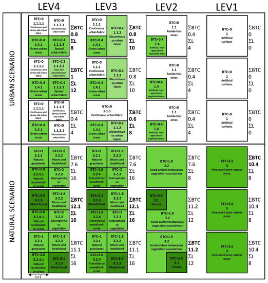
Figure 1.
Simplified landscape units representing six patterns of land cover across the four CORINE classification levels. Values represent the Biological Territorial Capacity (BTC value associated with each land cover (LC) (see Table A1, Appendix A). Green scale refers to BTC values of patches, with darker colors signifying higher ecological value. L represents the perimeter, i.e., the ecotonal zone of the LC patch with a BTC > 0. Higher values of ΣL describe more landscape diversity and the possibility of bio-energy exchange. Bold characters indicate higher total BTC and L values for each scenario.
The six scenarios of Figure 1 show that depending on the types of LC present in a landscape unit, the measures of bioenergy and length of the perimeter can vary across the CORINE level both in urban and natural scenarios: higher values of BTC can be revealed at the fourth, third or second CORINE thematic levels. To understand the relative impact on landscape connectivity of this hypothesis and, in general, of the change in thematic resolution of the LULC map, we propose to compare four thematic resolutions in a real study case using the PANDORA model (see Section 3).
3. Materials and Methods
The following Section 3.1 describes the PANDORA model. The study case is reported in Section 3.2, while Section 3.3 accounts for the data preparation and conducted assessments.
3.1. PANDORA Model
PANDORA is a “species-agnostic” modeling approach aiming to investigate the structural landscape connectivity [24,36,37]. The model integrates thermodynamic concepts, mathematical equilibrium, landscape metrics, graph, and metabolic theory [4,21,22]. The model assumes that solar energy feeds ecosystems that in turn release bioenergy through metabolism creating organized low-entropy structures [38,39]. The BTC index of vegetation metabolism is used to describe the bio-energy of each LULC patch, i.e., the flux of energy (Mcal/m2/year) that the ecological system has to dissipate in the environment to maintain its level of metastability [4]. Such bio-energy flows across the landscape and landscape elements can be limited by natural and anthropic barriers. Significant barriers to bio-energy fluxes define sub-systems called Bio-Energy Landscape Units (BELUs). PANDORA simulates the bio-energy of each BELU and the fluxes of bio-energy between adjacent BELUs using the so-called Bio-Energy Landscape Graph (BELG). The BELG, and the data used to build it, is used in the PANDORA algorithm, and by iterative computation, it calculates the mathematically asymptotic bio-energy metastable state related to a specific landscape pattern. Such an asymptotic value of bio-energy (Mas) is the PANDORA index of Bio-Energy Landscape Connectivity (BELC). Changes in the landscape pattern and factors affecting vegetational metabolism (i.e., climate, exposition, soil) that have an impact on the BELC can be measured by Mas. Moreover, PANDORA version 3.0 provides for each considered LULC patch a connectivity index (dMtot) and an ecosystem service value index for biodiversity conservation (ESV) (see Appendix B for a detailed description). The dMtot index is related to the contribution of each patch to the overall BELC. The dMtot index ranges between 0 and 100, where 100 indicates the greater contribution to BELC. The ESV index refers to the estimated ecosystem service value for biodiversity conservation of each patch, considering its habitat (i.e., LC), extension (m2), and contribution to BELC (i.e., dMtot index). The ESV can be expressed in monetary or non-monetary form. The PANDORA 3.0 model is a free and open-source plugin working on QGIS v.2.16 or earlier. Interestingly, PANDORA 3.0 uses a SQlite database for BTC values and value coefficients for ESV calculation based on the CORINE classification system. This feature makes the tool very helpful for testing different scenarios of thematic resolution. A full description of the PANDORA 3.0 model can be found in [21,22].
The PANDORA model has been used in different environmental planning contexts such as the scenario assessment of urban sprawl [4] and road development [40], or the planning of agricultural parks [22], eco-passages [41], and forestation areas [42]. The PANDORA model has been also applied in the assessment of the territorial resilience in the Douro Valley (Portugal) [43] and in the integrated spatial planning of the Parc Naturel Régional de la Montagne de Reims (France) [44]. In particular, the PANDORA version 3.0, with the possibility to also evaluate single patches in terms of ecosystem services, finds applications in urban green infrastructure planning. Pelorosso et al. (2016,2017) [21,22] used PANDORA 3.0 to evaluate the contribution of non-urbanized areas to landscape connectivity in Bari City (south Italy). Wanghe et al. (2019, 2020) [45,46] assessed urban green spaces in Tongzhou District (Beijing, China) to achieve a sustainable development strategy. The effects of land-use change and urbanization on ecosystem services for biodiversity conservation have been studied by PANDORA 3.0 in Xishuangbanna city [47] and Yunnan Province (Southwest China) [48].
3.2. Study Case
The study case is a strongly urbanized territory in the metropolitan area of Bari (Southern Italy) (Figure 2). The study area corresponds to the landscape unit known as “La Conca”, defined by the Apulia Region Territorial Landscape Plan. The extension of this territory (43.4 km2) has been previously evaluated as the best scale for landscape connectivity analysis to support sustainable urban development of the Bari city and adjacent municipalities [21]. The past and present urbanization phenomena and the growth of agricultural areas have strongly reduced naturalistic features that now are limited in the so-called Lame, natural incisions that form ephemeral rivers after heavy rainfalls [49]. The rural landscape is characterized by remaining agricultural patches intertwined with settlements, intensive cultivation of olive trees and table grapes [50]. The Lame represent, therefore, the most important connection systems from an ecological point of view, since they are characterized by the presence of spontaneous vegetation in an intensely cultivated and urbanized context.
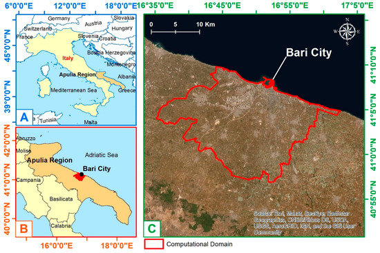
Figure 2.
Case Study “La Conca” in the metropolitan area of Bari (Southern Italy).
3.3. Data Preparation and Scenarios Assessment
In this work, four scenarios of thematic resolution have been tested by the PANDORA 3.0 model corresponding to the four levels of CORINE classification systems, namely LEV1, LEV2, LEV3, and LEV4, respectively. According to the conceptual scheme of Figure 1, the spatial resolution of the maps was maintained as fixed, but the polygons were dissolved to join adjacent LC patches having the same class. The base LULC map used in this study is the Apulia Region LULC map (scale 1:5000, Minimum Map Unit 2500 m2, 1600 m2 for urban areas) that is compliant with the standard CORINE classification system, fourth level (see Appendix A). The LULC map was produced in 2008 and updated in 2011 increasing the thematic information [21]. The BTC index has been associated with each land cover class considering previous literature and a downscaling methodology of calculation [4,21,22,40,51]. Starting from the BTC values assigned to LULC class of the third and fourth levels, the BTC indexes of the second and first levels have been calculated as the mean of the BTC index of the superior level. This procedure aims at maintaining coherence between levels considering an objective criterion of calculation. See Appendix A for the specific BTC values assigned to each LC.
The impact of thematic resolution variation on landscape connectivity was analyzed at two levels. The first level of analysis focuses on the BELC by investigating the variation of the Mas index at BELU and of the whole system. The second level of analysis regards 65 non-urbanized areas (NUAs) subjected to urban development and distributed across the study area. The aim of the NUA sample assessment was to highlight to what extent the thematic resolution affects the evaluation of similar patches (i.e., same original land cover: urban vegetated areas, BTC = 0.4) that are different in extension and spatial localization. The change in priority ranking of NUAs for conservation objectives was then analyzed according to the dMtot and ESV values (see Appendix B). In strongly urbanized areas, these indexes are usually small but the dMtot and ESV rank of NUA can support prioritization of interventions for conservation objectives and future sustainable urban expansion. A Kendall’s Tau-b coefficient was then computed between the four scenarios to test the similarity of ranks. In this work, ESV is expressed in non-monetary terms considering a value coefficient of 3 for all the NUAs [see 21]. Further model settings or details on NUAs can be found in Pelorosso et al. 2016 [21].
4. Results
Figure 3 shows the different distribution of BTC values assigned to the single land cover patches in the four scenarios of thematic aggregation. The image displays also the decreasing spatial resolution due to the aggregation of patches passing from the highest level (LEV4) to the lowest level (LEV1). The change in resolution of the patches can be also appreciated in Figure 4 by the K ecotope index at the BELU level. K ecotope index is an input parameter of PANDORA aimed at characterizing the bio-energy exchange among landcover patches with BTC >0. K ecotope takes into consideration the perimeter of the vegetated patches (the length of the ecotope zone where there is contact among different biotopes) and varies from 0 (no exchange) to 1 (maximum bioenergy exchange).
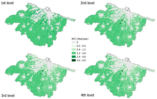
Figure 3.
BTC distribution among the four CORINE levels. See appendix A for detailed BTC values.
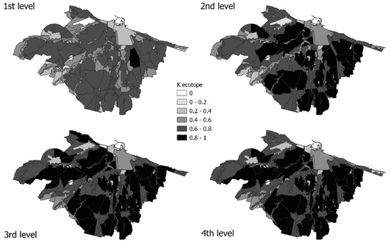
Figure 4.
Land cover patch diversity at (Bio-Energy Landscape Units) BELU level displayed by K ecotope. K ecotope is a PANDORA factor related to the perimeters (i.e., ecotone length) of vegetated land cover patches (BTC > 0).
4.1. Bio-Energy Landscape Connectivity Evaluation at BELU Level
Figure 5 shows the Bio-Energy Landscape Graphs (BELG) for the four scenarios. Small variations of bio-energy M (see also Table 1) and bio-energy fluxes can be observed among different CORINE levels, however, the effect of the LC thematic aggregation on the Bio-Energy Landscape Connectivity (BELC) is better described by the Asymptotic Generalized Biological Energy (Mas). Mas is the comprehensive PANDORA index of BELC and it represents the combined evaluation of land use, morphology, climate, anthropic and natural barriers. The graph in Figure 6 describes the evolution and the reaching of equilibrium values for each scenario relative to the Mas of all the systems (standardized value). LEV3 has the highest Mastot (0.17086), followed by LEV4 (0.17044), and they present similar evolution. Major differences in terms of evolution and equilibrium of Mastot among scenarios are in LEV1 (0.14354) and LEV2 (0.15641).
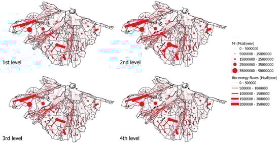
Figure 5.
Bio-Energy Landscape Graph (BELG). Circles represent the bio-energy of each BELU and arcs describe the fluxes of bio-energy between adjacent BELUs.

Table 1.
Comparison between couples of scenarios at the Bio-Energy Landscape Unit (BELU) level.
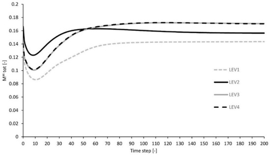
Figure 6.
Evolution and the reaching of equilibrium values for each scenario relative to the generalized bio-energy of all the systems’ Mastot (standardized values).
Figure 7 presents standardized Mas maps displaying the most important BELUs for the ecological functionality of the entire La Conca system. The diversity in the ranking of values among scenarios is also investigated by Tau-b statistics that describe the similarity of ordering among datasets (Table 1). The highest similarity among scenarios was found between LEV4 and LEV3 (Tau-b = 0.585, 0.990, 0.868, p < 0.01 for M, Mas, and K ecotope, respectively). In contrast, minor similarities have been identified between LEV4/LEV1 in terms of Mas (Tau-b = 0.894, p < 0.01), LEV2/LEV1 in terms of M (Tau-b = 0.369, p < 0.01), and LEV3/LEV1 in terms of K ecotope (Tau-b = 0.554, p < 0.01). Because small variations of Mas can be found among the scenarios, a study of the relative changes among BELUs is required to appreciate the effects of the different land cover aggregations. Figure 8 shows the change between couples of CORINE levels in terms of standardized Mas. Noteworthy is the minor Mas of several BELUs in LEV4 with respect to LEV3. Finally, the Normalized Root Mean Square Deviation (NRMSD) of Mas among scenarios is presented in Figure 9. NRMSD highlights the BELU variability among scenarios of thematic aggregation in terms of Mas. The effect of the thematic level change on Mas is evident in BELU no. 9, followed by BELU nos. 50, 42, 83, 174, 181, and 187.
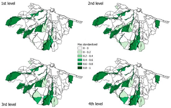
Figure 7.
Asymptotic Generalized Biological Energy (Mas)–standardized value. Note that each Masi is divided by the maximum M value for the specific BELUi.
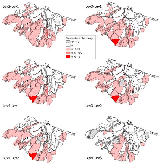
Figure 8.
Asymptotic Generalized Biological Energy (Mas) change between couples of CORINE levels–standardized values. Note that Mas changes are divided by the maximum Mas change among the six level comparison couples.
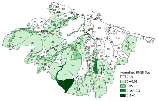
Figure 9.
Effects of the four (Land Use/Land Cover) LULC class aggregation on Bio-Energy Landscape Connectivity at BELU level: Normalized Root Mean Square Deviation (NRMSD) of asymptotic M.
4.2. Bio-Energy Landscape Connectivity Evaluation at the NUA Level
The LEV4 scenario, presenting the most detailed information about the land cover, is expected to be the optimal base layer for landscape connectivity assessment. A synthetic comparison of the 65 NUAs among the four scenarios is represented in Table 2 and Table 3. Table 2 shows data (mean, standard deviation, and maximum value of dMtot and ESV) related to each of the four scenarios, while Table 3 shows a direct comparison between pairs of scenarios (i.e., LEV2 vs. LEV1). The aim is to investigate the effect of the LULC category aggregation on NUA assessment, in particular with respect to the expected best level available for the analysis of landscape connectivity (i.e., LEV4). Interestingly, descriptive statistics of Table 2 show that the LEV3 scenario has the highest dMtot index while LEV4 presents the highest ESV values.
Table 2.
Land cover aggregation scenario comparison: descriptive statistics. Bold numbers represent maximum values.
Table 3.
Comparison between couples of scenarios at the Non-Urbanized Area (NUA) level. Bold numbers represent maximum values.
The comparison between coupled scenarios in Table 3 shows that the highest percentage increases for the values of dMtot mean and SD occur in scenario LEV2 with respect to LEV1. The couple LEV4/LEV3 presents a lower difference for average dMtot (−5.5%). This trend is reversed for average ESV values, where the difference between LEV4 and LEV3 is the greatest (+1.031%). Opposite trends between average dMtot and average ESVs are also revealed for the couples LEV3/LEV1 and LEV3/LEV2 where the average ESVs are −0.473% and −0.875%, respectively.
To highlight the closing or the distance of assessment among scenarios, the root mean squares deviations (RMSD) for both dMtot index and ESV values were computed. The RMSD confirms the greater dissimilarity between LEV3 and the other ones in terms of both the dMtot index and ESV; in particular, the highest difference is found in the couple LEV3/LEV1 (dMtot RMSD = 0.011, ESV RMSD = 11,454.8). The closer similarity is found in the couple LEV4/LEV2 (dMtot RMSD = 0.002, ESV RMSD = 174.7).
The assessment of NUAs in the four scenarios points out only small variations of indexes (see the low RMSD values in Table 3). The highest variations in real units (>|0.004| for dMtot and/or >|100| for ESV) were observed for the NUAs reported in Table 4 and Table 5, respectively. NUA no. 42 has the most variable evaluation in terms of dMtot (RMSD = 0.056) but it is stable for ESV across the scenarios (RMSD = 0). NUA no. 14 shows the highest ESV variation (RMSD = 56,719.292) with the major evaluation change between the LEV3 and LEV1 (ΔESV = −82,001.9).
Table 4.
Higher NUA assessment variations in real units (>|0.004| for dMtot) among scenarios. Bold numbers represent maximum absolute values.
Table 5.
Higher NUA assessment variations in real units (>|100| for ESV) among scenarios. Bold numbers represent maximum values.
Figure 10 shows the spatial distribution of the NUA in terms of dMtot and ESV for LEV4 scenario. It is noteworthy that the most important NUAs in terms of dMtot fall in the most important BELU for the overall ecological connectivity of La Conca. In contrast, some of the highest ESVs are associated with large NUAs, confirming the weight of the area in the calculation of the ESV (see Appendix B, Equation (A2)).
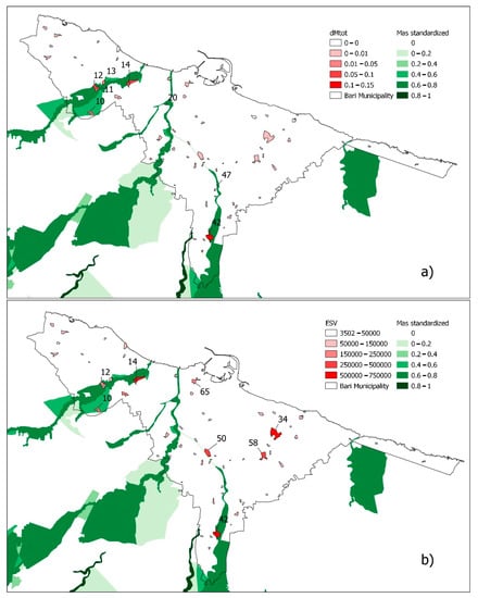
Figure 10.
Spatial visualization of NUA assessment using CORINE fourth level thematic aggregation. (a) dMtot index; (b) Ecosystem Service Value (ESV) for biodiversity conservation. Numbers represent the ID of the first ranked NUAs.
The NUA priority ranking among scenarios was evaluated by Kendall’s Tau-b statistic (Table 3). The highest similarity of ordering among datasets in terms of dMtot was found between scenarios LEV4 and LEV3 (Tau-b = 0.945, p < 0.01), followed by the couples of scenarios LEV3/ LEV2 (Tau-b = 0.902, p < 0.01) and LEV4/ LEV2 (Tau-b = 0.886, p < 0.01). In contrast, no appreciable change in priority ranking in terms of ESV was identified by the Tau-b statistic, the circumstance that confirms the strongest similarity of the couple LEV4/LEV2 (Tau-b = 0.999, p < 0.01).
Table 6 and Table 7 show the ranking difference among scenarios (respectively the dMtot and ESV ranking) where the first ten NUAs of LEV4 were taken as the reference for the comparison. NUA no. 42 was identified as the most important patch in terms of dMtot index and ESVs in all four scenarios. NUA no. 14 results in all scenarios at second and third position for dMtot and ESV, respectively. The first nine positions are stable in LEV2, LEV3, and LEV4 in terms of dMtot, while LEV1 presents an alteration of NUA ranking starting from the third position. Looking at the ESV ranking, the assessment shows greater robustness across the LC category level. Indeed, the ranking of the first five NUAs of LEV4 is confirmed at the scale of LEV1, LEV2, and LEV3.
Table 6.
NUA ranking in terms of the dMtot. The bold value represents the NUAs rank that shows the correspondence between the scenarios (LEV1, LEV2, LEV3) and the LEV4.
Table 7.
NUA ranking in terms of the ESV. The bold value represents the NUAs rank that shows the correspondence between the scenarios (LEV1, LEV2, LEV3) and the LEV4.
5. Discussions
5.1. Thematic Resolution and Bioenergy Landscape Connectivity
The obtained results show that variability of connectivity measures exist within the four thematic resolutions of the LC map corresponding to the four levels of the CORINE classification system (i.e., LEV1, LEV2, LEV3, and LEV4 scenarios).
The most detailed thematic resolution (LEV4) is expected to display a better representation of the habitats and landscape patterns. As consequence, LEV4 should be considered the most tailored data for simulating the actual ecological fluxes in terms of bio-energy, followed by LEV3, LEV2, and LEV1. However, the analysis at the whole landscape scale reveals that the Mastot of LEV3 is very similar to LEV4 (Figure 6). Indeed, LEV3 and LEV4 have strong similarities, as verified by the assessment conducted at the BELU level (Figure 7 and Table 1). The small difference between LEV3 and LEV4 can be also explained by the similar K ecotope values, the landscape metric related to the mosaic fragmentation, and bio-energy exchanges among LC patches (Figure 4 and Table 1). Besides that, LEV4 shows lower Mas values in several BELUs with respect to LEV3 (Figure 8). This phenomenon highlights that a higher thematic resolution is not always related to higher landscape connectivity.
The conceptual scheme of Figure 1 asserts that the spatial distribution of LC classes could affect connectivity evaluation more than a change in thematic resolution. While the scheme of Figure 1 shows a hypothetical isolated system, the presented results derive from the modeling of multiple bio-energy fluxes among landscape units. The variability of Mas confirms therefore that the hypothesis of Figure 1 is verified also in a real landscape connectivity case study, where the interactions between ecological systems (i.e., BELUs) are considered. Moreover, it is noteworthy that some BELUs present a higher variability of Mas values across the four scenarios (BELU no. 9, 50, 42, 83, 174, 181, and 187). Moreover, these unstable BELUs have ecological importance for the BELC of the whole system as they are in, or they are close to, the Lame system (see Figure 9). Consequently, the results prove that the thematic resolution of the LULC map can determine hotspots of landscape connectivity changes.
To understand if these global and local variations of BELC could significantly alter environmental evaluations in planning decisions, the analysis has been focused on a sample of areas distributed among the BELUs. In particular, the assessment aimed at revealing evaluation changes of a set of non-urbanized areas (NUAs) that could be developed in future urban expansions. Each NUA has been evaluated in terms of the dMtot and ESV that express the importance of the NUA for biodiversity conservation in terms of connectivity index and ecosystem service value, respectively. In general, indexes present small variations in NUAs across the four scenarios but with a varied pattern of values that deserves to be discussed. LEV3 scenario displays the highest dMtot index and the lowest ESV; LEV4 presents the highest ESV values and the lowest dMtot index (see Table 2). The comparison among couples of scenarios (Table 3) reveals the highest percentage difference of the dMtot index when considering LEV1: In this first level, the simplification of the landscape mosaic and the assigned BTC values have reduced the dMtot index of some NUAs nearly to zero; consequently, the average percentage variation of dMtot index between LEV1 and the other levels are very high. The dMtot index in the coupled scenarios LEV4/LEV3 presents the lower average percentage difference (Δ%dMtot = −5.5%) but the highest difference in real values (dMtot RMSD = 0.011). It is noteworthy that very small variations of dMtot exist across the four scenarios as the dMtot index ranges between 0 and 100. In contrast, ESV evaluation displays a minor average percentage difference with the higher changes between LEV4 and LEV3 (+1.031%). The other couples of scenarios present a certain variability of values making it difficult to define a clear lecture of the results. For example, the average ESV of the NUAs is smaller in LEV3 than LEV2 or LEV1, while, surprisingly, the more similar scenarios appear in the couple LEV4/LEV2 (dMtot RMSD = 0.002; ESV RMSD = 174.7).
These results highlight that the thematic resolution has a potential impact on the BELC, nevertheless a direct relationship among the number of LC classes and landscape connectivity does not exist and the spatial pattern of LC can strongly influence the final evaluations. Indeed, PANDORA indexes significantly vary in a few NUAs (see Table 4 and Table 5). To understand if these variations of the dMtot and ESV could affect the planning decision, a further evaluation has been carried out in NUA priority ranking for conservation actions. In general, rankings of NUA present a limited change across scenarios of thematic resolution with a higher stability of ESV ranking compared to the dMtot ranking (see Table 3, Tau-b statistics). However, the results show that the thematic resolution can determine errors in the identification of the priority of intervention. Indeed, taking into consideration LEV4 as the reference, several NUAs change position in the rankings (Table 6 and Table 7). The rankings that are based only on measures of landscape connectivity (i.e., the dMtot index) present certain stability for the LEV2, LEV3, and LEV4 within the first nine positions, while the LEV1 ranking starts to change from the third position. The ESV rankings are more stable in all four scenarios with priority changes in LEV1 and LEV3 after the fifth position. The higher stability of the ESV ranking is due to the formulation of indicators that relies on the integration of dMtot, the LC type, and the extension of the patch [21,22].
5.2. Limitations and Future Developments
The PANDORA model is based on a “species-agnostic”, or top-down, structural landscape connectivity approach usually proposed for management and planning purposes [24,36,37]. This approach considers mainly the degree of naturalness and human intervention and how these features interact with physical processes. A wide range of thematic classes of CORINE land cover can be employed in PANDORA thanks to the compatibility of the SQlite database inside the model and the possibility to assign a bio-energy value (BTC index) for each LC class until the fourth level. This possibility has allowed testing a large set of thematic resolution changes across different artificial, seminatural, and natural LC classes.
It is noteworthy that an evaluation focused on specific species could require a different modeling approach, such as least-cost path analysis, circuit theory, matrix theory, agent or individual-based modeling [21,25,26], or more detailed information on specific vegetation types, habitats, and landscape features [27].
The proposed BTC values are assigned with a logical criterion across the four CORINE thematic levels. The connectivity measures could vary by adopting different BTC assignment criteria or BTC values for specific LC classes. However, we argue that, according to [35], measured BELC would not be sensitive to the thematic resolution if the rank order of BTC values is maintained across LC classes. Indeed, connectivity estimates are usually robust against errors in cost values associated with LC classes, as the overall rank-order of the cost values remains consistent [33]. It is noteworthy that uncertainty in connectivity estimates is inevitable, as the data available often are limited, incomplete, or out-of-date [33].
From this point of view, a measure of uncertainty would be desirable. As an example, the underlying continuous variability of land cover classes could be mapped based on fuzzy sets theory [52]. In most cases, boolean membership is often used to create LULC maps by thresholding the original data based on a maximum likelihood criterion. On the contrary, the landscape under study has a continuous variability of LC in space. Hence, a fuzzy membership might be used by considering the possibility for each pixel to attain a certain class, by further creating a map for each class with membership possibilities for each entity (e.g., each pixel) [53].
Besides the boolean idea under the CORINE scheme, a further problem is mainly related to anthropogenic classes. A classification related to the underlined ecosystem processes, e.g., vegetation dynamics, would lead to better ecological insights. This caveat would lead to the conclusion that LC classes-related diversity is not always related to biodiversity in the field. This is still an open question in the literature [27]. However, the LC heterogeneity estimate would be the first exploratory tool to further guide the field-based studies to inspect in situ diversity. From this point of view, historical data, providing information on LC classes as well as the management of the different areas, could be beneficial for the effective planning of further management practices.
Finally, the LULC thematic resolution is expected to affect several environmental evaluations, consequently, similar studies deserve to be realized in different research fields in the future. For example, investigating the thematic resolution impact on hydrological modeling [54] and related research topics, such as soil erosion, sediment transport [55], and hydraulic risk [56].
6. Conclusions
Which is the best LULC thematic resolution for environmental assessment and land use planning? The present paper aims at addressing this issue, evaluating the possible impact of different thematic resolutions on landscape connectivity assessment, a crucial environmental aspect for biodiversity conservation. Answering the question is not easy, because several variables play a role in the final decision. The modeling approaches, the considered species, the availability of data and resources to produce LULC maps with a suitable spatial resolution are some of the factors that surely affect the choice of the thematic resolution of the map. The present manuscript presents the landscape connectivity assessment of four scenarios with increasing thematic resolution (namely, LEV1, LEV2, LEV3, and LEV4) corresponding to the four CORINE levels in an urban context of southern Italy. The PANDORA 3.0 model was used to evaluate Bio-Energy Landscape Connectivity (BELC) based on bio-energy fluxes among landscape units. Scenarios comparison was investigated through the indicators of landscape connectivity and ecosystem services working at three scales: the largest (whole system), the middle (Bio-Energy Landscape Unit), and the smallest one (land cover patch). The results show that with a fixed spatial resolution:
- The thematic resolution has a potential impact on the BELC but a direct relation between the number of LC classes and landscape connectivity measures does not exist.
- The higher thematic resolution is not always related to the higher measure of landscape connectivity, but LEV1 strongly differs from the other more detailed levels.
- The spatial distribution of LC classes can affect connectivity evaluation more than the change in thematic resolution.
- The changes in thematic resolution of the LULC map can determine hotspots of landscape connectivity changes.
- The changes in thematic resolution can determine errors in the identification of priority of intervention.
- The proposed index of ecosystem services provides a more stable ranking of conservation priority among different thematic resolutions.
In conclusion, we demonstrated that the thematic resolution of the LULC map impacts the landscape connectivity evaluation due to the spatial pattern of the LULC classes. Researchers and practitioners, when choosing thematic resolution, should be aware of the possible misleading assessment that is synthetically aforementioned. Moreover, measures of ecosystem services that integrate connectivity index with other ecological features could be preferred to reduce the erroneous evaluation of priority ranking for conservation objectives. Further efforts are required to investigate the impact of thematic resolution and LC classification types (e.g., fuzzy map) on different approaches to landscape connectivity (e.g., functional connectivity), and on different environmental processes (e.g., hydrological and hydraulic modeling).
Author Contributions
Conceptualization, R.P.; data gathering and methodology, R.P.; data processing, R.P.; writing—original draft preparation, review and editing of the final document by all authors; figures and tables, R.P., C.A. All authors have read and agreed to the published version of the manuscript.
Funding
This research received no external funding.
Institutional Review Board Statement
Not Applicable.
Informed Consent Statement
Not Applicable.
Data Availability Statement
The data presented in this study are available on request from the corresponding author.
Conflicts of Interest
The authors declare no conflict of interest.
Appendix A
Table A1.
Thematic levels of CORINE land cover system and BTC index.
Table A1.
Thematic levels of CORINE land cover system and BTC index.
| 1st Level | BTC Index1 (Mcal/m2/year) | 2nd Level | BTC Index2 (Mcal/m2/year) | 3rd Level | BTC Index3 (Mcal/m2/year) | 4th Level | BTC Index4 (Mcal/m2/year) |
|---|---|---|---|---|---|---|---|
| 1. ARTIFICIAL SURFACES | 0 | 1.1 Residential areas | 0 | 1.1.1 Continuous urban fabric | 0 | 1.1.1.1 Continuous and dense old urban fabric | 0 |
| 1.1.1.2 Continuous, dense and recent low urban fabric | 0 | ||||||
| 1.1.1.3 Continuous, dense and recent high urban fabric | 0 | ||||||
| 1.1.2 Discontinuous urban fabric | 0.2 * | 1.1.2.1 Discontinuous urban fabric | 0 | ||||
| 1.1.2.2 Rare and discontinuous urban fabric | 0.2 * | ||||||
| 1.1.2.3 Sprawl urban fabric | 0.4 * | ||||||
| 1.2 Industrial, commercial and transport units | 0 | 1.2.1 Industrial or commercial units | 0 | 1.2.1.1 Industrial units | 0 | ||
| 1.2.1.2 Commercial units | 0 | ||||||
| 1.2.1.3 Public and private service facilities | 0 | ||||||
| 1.2.1.4 Hospitals | 0 | ||||||
| 1.2.1.5 Techonological sites | 0 | ||||||
| 1.2.1.6 Farm facilities | 0 | ||||||
| 1.2.1.7 Abandoned sites | 0 | ||||||
| 1.2.2 Road and rail networks and associated land | 0 | 1.2.2.1 Roads networks | 0 | ||||
| 1.2.2.2 Railways networks | 0 | ||||||
| 1.2.2.3 Goods storage and marshalling facilities | 0 | ||||||
| 1.2.2.4 Telecommunication facilities | 0 | ||||||
| 1.2.2.5 Areas and networks for the distribution, production and transport of energy | 0 | ||||||
| 1.2.3 Port areas | 0 | ||||||
| 1.2.4 Airports | 0 | ||||||
| 1.3 Mine, dump and construction sites | 0 | 1.3.1 Mineral extraction sites | 0 | ||||
| 1.3.2 Dump sites and mine deposits | 0 | 1.3.2.1 Dump and mine deposits with an extension greater than 0.5 ha | 0 | ||||
| 1.3.2.2 Dumps and car demolition sites | 0 | ||||||
| 1.3.3 Construction sites | 0 | 1.3.3.1 Construction sites | 0 | ||||
| 1.3.3.2 Artificial soils | 0 | ||||||
| 1.4 Artificial, non-agricultural vegetated areas | 0.4 | 1.4.1 Green urban areas | 0.4 | ||||
| 1.4.2 Sport and leisure facilities | 0.4 | 1.4.2.1 Camping areas, bungalows and other accomodotion facilities | 0.4 | ||||
| 1.4.2.2 Sport facilities | 0.4 | ||||||
| 1.4.2.3 Leisure facilities | 0.4 | ||||||
| 1.4.2.4 Archeological sites | 0.4 | ||||||
| 1.4.3 Cemeteries ** | 0.4 | ||||||
| 2. AGRICULTURAL AREAS | 1.3 * | 2.1 Arable land | 0.9 * | 2.1.1 Non-irrigated arable land | 0.8 * | 2.1.1.1 Non irrigated arable land | 1 |
| 2.1.1.2 Field or greenhouse horticulture in non irrigated arable land | 0.7 | ||||||
| 2.1.2 Permanently irrigated land | 1 * | 2.1.2.1 Permanently irrigated arable land | 1.2 * | ||||
| 2.1.2.3 Field or greenhouse horticulture in permanently irrigated arable land | 0.8 | ||||||
| 2.1.3 Rice fields | 0.8 | ||||||
| 2.2 Permanent crops | 1.8 | 2.2.1 Vineyards | 1.5 | ||||
| 2.2.2 Fruit trees and berry plantations | 1.5 | ||||||
| 2.2.3 Olive groves | 1.5 | ||||||
| 2.2.4 Other permanent crops ** | 2.6 | ||||||
| 2.3 Pastures | 1 | 2.3.1 Pastures | 1 | ||||
| 2.4 Heterogeneous agricultural areas | 1.6 * | 2.4.1 Annual crops associated with permanent crops | 1 | ||||
| 2.4.2 Complex cultivation patterns | 1.6 | ||||||
| 2.4.3 Land principally occupied by agriculture, with significant areas of natural vegetation | 1.8 | ||||||
| 2.4.4 Agro-forestry areas | 2 | ||||||
| 3. FOREST AND SEMI NATURAL AREAS | 2.6 | 3.1 Forests | 5.5 | 3.1.1 Broad-leaved forest | 6.5 | ||
| 3.1.2 Coniferous forest | 5.5 | ||||||
| 3.1.3 Mixed forest | 5.5 | ||||||
| 3.1.4 Pastures with perennial plants ** | 5 | ||||||
| 3.2 Scrub and/or herbaceous vegetation associations | 1.9 * | 3.2.1 Natural grasslands | 1 | ||||
| 3.2.2 Moors and heathland | 1.8 | ||||||
| 3.2.3 Sclerophyllous vegetation | 2 | ||||||
| 3.2.4 Transitional woodland-scrub | 2.8 | 3.2.4.1 Natural recolonization areas | 2.8 | ||||
| 3.2.4.2 Artificial recolonization areas (reforestation) | 2.8 | ||||||
| 3.3 Open spaces with little or no vegetation | 0.3 * | 3.3.1 Beaches, dunes, sands | 0 | ||||
| 3.3.2 Bare rocks | 0 | ||||||
| 3.3.3 Sparsely vegetated areas | 0.6 | ||||||
| 3.3.4 Burnt areas or areas damaged by other causes | 0.8 | ||||||
| 3.3.5 Glaciers and perpetual snow | 0 | ||||||
| 4. WETLANDS | 0.3 | 4.1 Inland wetlands | 0.3 | 4.1.1 Inland marshes | 0.3 | ||
| 4.1.2 Peat bogs | 0.3 | ||||||
| 4.2 Maritime wetlands | 0.3 | 4.2.1 Salt marshes | 0.3 | ||||
| 4.2.2 Salines | 0.3 | ||||||
| 4.2.3 Intertidal flats | 0.3 | ||||||
| 5. WATER BODIES | 0.1 | 5.1 Inland waters | 0.1 | 5.1.1 Water courses | 0 | 5.1.1.1 Rivers and streams | 0 |
| 5.1.1.2 Channels and waterways | 0 | ||||||
| 5.1.2 Water bodies | 0.3 | 5.1.2.1 Water bodies | 0.3 | ||||
| 5.1.2.2 Water bodies for irrigation purpose | 0.3 | ||||||
| 5.1.2.3 Aquaculture | 0.3 | ||||||
| 5.2 Marine waters | 0.2 * | 5.2.1 Coastal lagoons | 0.3 | ||||
| 5.2.2 Estuaries | 0.3 | ||||||
| 5.2.3 Sea and ocean | 0 |
* Variation of BTC index with respect to the current SQLITE database in PANDORA 3.0 plugin. ** 3rd level CORINE classes present only in the Apulia land use map.
Appendix B
PANDORA 3.0 uses an algebraic hierarchy and an approximated solution of the fundamental Ordinary Differential Equations (ODEs) to calculate the final asymptotic energetic equilibrium of each patch j belonging to a Bio-Energy Landscape Unit i (BELUi). The patch evolution is then regulated by several factors related to the metabolism (i.e., BTC index), the barriers to Bio-Energy fluxes inside the BELUi and the connectivity among BELUs. The asymptotic Bio-Energy of the BELUi (Masi) is derived from the asymptotic Bio-Energy of the patches j, adjusted by some specific K parameters related to the patch ecotones, climate, solar exposition and soil type of the BELUi. The Generalized Bio-Energy of the overall system Mastot is finally calculated as the sum of all the Masi.
The dMtot index evaluates the contribution of each patch to the overall Bio-Energy Landscape Connectivity (BELC). It is calculated as follows:
where Mastotj is the Generalized Bio-Energy of the overall system that considers the asymptotic values of all the patches j under the existing barriers to energy fluxes, climatic, morphological and soil conditions.
dMtotkj indicates the importance of each patch j and land cover category k in terms of its contribution to the maintenance of the overall BELC by comparing the overall connectivity difference before (i.e., Mastotj) and after (i.e., Mastot’j) changing patch j into an urban area (i.e., impervious with no photosynthetic surface and BTC index = 0). dMtot ranges between 0 and 100, where 100 means a total BELC reduction after urbanising the patch.
The ESV index describes the Ecosystem Services Value for biodiversity conservation of a patch considering the connectivity measure described by the dMtot index, its extension and LC type as follows:
where ESVjk is the Ecosystem Services Value for biodiversity conservation of a singular patch j of land cover category k, Aj is the area (m2) of the patch j, dMtotj_max indicates the maximum value of dMtot among all the analysed patches j of the landscape without considering land cover type difference. VCk is the value coefficient for biodiversity conservation of the land cover category k. VCk can be expressed in monetary or non-monetary form. The PANDORA 3.0 model plugin reports VC default values for supporting biodiversity in the scale 0–5 [22]. Then, ESV_B defines an increased value (which can be as high as double the original value) for patches significantly important for the BELC (high dMtot index) with respect to the evaluation that considers only habitat type (land cover) and area of the patches.
References
- Song, X.P.; Hansen, M.C.; Stehman, S.V.; Potapov, P.V.; Tyukavina, A.; Vermote, E.F.; Townshend, J.R. Global land change from 1982 to 2016. Nature 2018, 560, 639–643. [Google Scholar] [CrossRef]
- Creutzig, F.; Bren D’Amour, C.; Weddige, U.; Fuss, S.; Beringer, T.; Gläser, A.; Kalkuhl, M.; Steckel, J.C.; Radebach, A.; Edenhofer, O. Assessing human and environmental pressures of global land-use change 2000–2010. Glob. Sustain. 2019, 2, e1. [Google Scholar] [CrossRef]
- Pelorosso, R.; Leone, A.; Boccia, L. Land cover and land use change in the Italian central Apennines: A comparison of assessment methods. Appl. Geogr. 2009, 29, 35–48. [Google Scholar] [CrossRef]
- Gobattoni, F.; Pelorosso, R.; Lauro, G.; Leone, A.; Monaco, R. A procedure for mathematical analysis of landscape evolution and equilibrium scenarios assessment. Landsc. Urban Plan. 2011, 103, 289–302. [Google Scholar] [CrossRef]
- Recanatesi, F.; Petroselli, A. Land Cover Change and Flood Risk in a Peri-Urban Environment of the Metropolitan Area of Rome (Italy). Water Resour. Manag. 2020, 34, 4399–4413. [Google Scholar] [CrossRef]
- Petrisor, A.I.; Sirodoev, I.; Ianos, I. Trends in the national and regional transitional dynamics of land cover and use changes in Romania. Remote Sens. 2020, 12, 230. [Google Scholar] [CrossRef]
- Apollonio, C.; Balacco, G.; Novelli, A.; Tarantino, E.; Piccinni, A.F. Land use change impact on flooding areas: The case study of Cervaro Basin (Italy). Sustainability 2016, 8, 996. [Google Scholar] [CrossRef]
- Lechner, A.M.; Rhodes, J.R. Recent Progress on Spatial and Thematic Resolution in Landscape Ecology. Curr. Landsc. Ecol. Rep. 2016, 1, 98–105. [Google Scholar] [CrossRef]
- Grafius, D.R.; Corstanje, R.; Warren, P.H.; Evans, K.L.; Hancock, S.; Harris, J.A. The impact of land use/land cover scale on modelling urban ecosystem services. Landsc. Ecol. 2016, 31, 1509–1522. [Google Scholar] [CrossRef]
- García-Álvarez, D.; Lloyd, C.D.; Van Delden, H.; Camacho Olmedo, M.T. Thematic resolution influence in spatial analysis. An application to Land Use Cover Change (LUCC) modelling calibration. Comput. Environ. Urban Syst. 2019, 78, 101375. [Google Scholar] [CrossRef]
- Giri, C.P. Remote Sensing of Land Use and Land Cover. Principles and Applications; CRC Press: Boca Raton, FL, USA, 2012; ISBN 9781420070750. [Google Scholar]
- Gennaretti, F.; Ripa, M.N.; Gobattoni, F.; Boccia, L. A methodology proposal for land cover change analysis using historical aerial photos. J. Geogr. Reg. Plan. 2011, 4, 542–556. [Google Scholar]
- Lee, J.; Cardille, J.A.; Coe, M.T. BULC-U: Sharpening resolution and improving accuracy of land-use/land-cover classifications in Google Earth Engine. Remote Sens. 2018, 10, 1455. [Google Scholar] [CrossRef]
- Tassi, A.; Vizzari, M. Object-oriented lulc classification in google earth engine combining snic, glcm, and machine learning algorithms. Remote Sens. 2020, 12, 3776. [Google Scholar] [CrossRef]
- Amici, V.; Marcantonio, M.; La Porta, N.; Rocchini, D. A multi-temporal approach in MaxEnt modelling: A new frontier for land use/land cover change detection. Ecol. Inform. 2017, 40, 40–49. [Google Scholar] [CrossRef]
- Bailey, D.; Billeter, R.; Aviron, S.; Schweiger, O.; Herzog, F. The influence of thematic resolution on metric selection for biodiversity monitoring in agricultural landscapes. Landsc. Ecol. 2007, 22, 461–473. [Google Scholar] [CrossRef]
- Anderson, J.R.; Hardy, E.E.; Roach, J.T.; Witmer, E. A Land Use and Land Cover Classification System for Use with Remote Sensor Data; US Government Printing Office: Washington, DC, USA, 1976; Volume 964.
- Büttner, G.; Kostztra, B.; Soukup, T.; Sousa, A.; Langanke, T. CLC2018 Technical Guidelines; European Environment Agency: Copenhagen, Denmark, 2017; pp. 1–60. [Google Scholar]
- Martínez-Fernández, J.; Ruiz-Benito, P.; Bonet, A.; Gómez, C. Methodological variations in the production of CORINE land cover and consequences for long-term land cover change studies. The case of Spain. Int. J. Remote Sens. 2019, 40, 8914–8932. [Google Scholar] [CrossRef]
- Varga, O.G.; Pontius, R.G.; Szabó, Z.; Szabó, S. Effects of category aggregation on land change simulation based on corine land cover data. Remote Sens. 2020, 12, 1314. [Google Scholar] [CrossRef]
- Pelorosso, R.; Gobattoni, F.; Geri, F.; Monaco, R.; Leone, A. Evaluation of Ecosystem Services related to Bio-Energy Landscape Connectivity (BELC) for land use decision making across different planning scales. Ecol. Indic. 2016, 61, 114–129. [Google Scholar] [CrossRef]
- Pelorosso, R.; Gobattoni, F.; Geri, F.; Leone, A. PANDORA 3.0 plugin: A new biodiversity ecosystem service assessment tool for urban green infrastructure connectivity planning. Ecosyst. Serv. 2017, 26, 476–482. [Google Scholar] [CrossRef]
- Pascual-Hortal, L.; Saura, S. Impact of spatial scale on the identification of critical habitat patches for the maintenance of landscape connectivity. Landsc. Urban Plan. 2007, 83, 176–186. [Google Scholar] [CrossRef]
- Marrec, R.; Abdel Moniem, H.E.; Iravani, M.; Hricko, B.; Kariyeva, J.; Wagner, H.H. Conceptual framework and uncertainty analysis for large-scale, species-agnostic modelling of landscape connectivity across Alberta, Canada. Sci. Rep. 2020, 10, 6798. [Google Scholar] [CrossRef] [PubMed]
- Babí Almenar, J.; Bolowich, A.; Elliot, T.; Geneletti, D.; Sonnemann, G.; Rugani, B. Assessing habitat loss, fragmentation and ecological connectivity in Luxembourg to support spatial planning. Landsc. Urban Plan. 2019. [Google Scholar] [CrossRef]
- Pierik, M.E.; Matteo, D.; Confalonieri, R.; Bocchi, S.; Gomarasca, S. Designing ecological corridors in a fragmented landscape: A fuzzy approach to circuit connectivity analysis. Ecol. Indic. 2016, 67, 807–820. [Google Scholar] [CrossRef]
- Kallimanis, A.S.; Koutsias, N. Geographical patterns of Corine land cover diversity across Europe: The effect of grain size and thematic resolution. Prog. Phys. Geogr. 2013, 37, 161–177. [Google Scholar] [CrossRef]
- Rocchini, D. Effects of spatial and spectral resolution in estimating ecosystem α-diversity by satellite imagery. Remote Sens. Environ. 2007, 111, 423–434. [Google Scholar] [CrossRef]
- Marshall, L.; Beckers, V.; Vray, S.; Rasmont, P.; Vereecken, N.J.; Dendoncker, N. High thematic resolution land use change models refine biodiversity scenarios: A case study with Belgian bumblebees. J. Biogeogr. 2021, 48, 345–358. [Google Scholar] [CrossRef]
- Seoane, J.; Bustamante, J.; Díaz-Delgado, R. Are existing vegetation maps adequate to predict bird distributions? Ecol. Modell. 2004, 175, 137–149. [Google Scholar] [CrossRef]
- Cushman, S.A.; Landguth, E.L. Scale dependent inference in landscape genetics. Landsc. Ecol. 2010, 25, 967–979. [Google Scholar] [CrossRef]
- Zeller, K.A.; McGarigal, K.; Cushman, S.A.; Beier, P.; Vickers, T.W.; Boyce, W.M. Sensitivity of resource selection and connectivity models to landscape definition. Landsc. Ecol. 2017, 32, 835–855. [Google Scholar] [CrossRef]
- Simpkins, C.E.; Dennis, T.E.; Etherington, T.R.; Perry, G.L.W. Effects of uncertain cost-surface specification on landscape connectivity measures. Ecol. Inform. 2017, 38, 1–11. [Google Scholar] [CrossRef]
- Amici, A.; Pelorosso, R.; Serrani, F.; Boccia, L. A nesting site suitability model for rock partridge (Alectoris graeca) in the Apennine Mountains using logistic regression. Ital. J. Anim. Sci. 2009, 8, 751–753. [Google Scholar] [CrossRef][Green Version]
- Bowman, J.; Adey, E.; Angoh, S.Y.J.; Baici, J.E.; Brown, M.G.C.; Cordes, C.; Dupuis, A.E.; Newar, S.L.; Scott, L.M.; Solmundson, K. Effects of cost surface uncertainty on current density estimates from circuit theory. PeerJ 2020, 8, e9617. [Google Scholar] [CrossRef]
- Dickson, B.G.; Albano, C.M.; Anantharaman, R.; Beier, P.; Fargione, J.; Graves, T.A.; Gray, M.E.; Hall, K.R.; Lawler, J.J.; Leonard, P.B.; et al. Circuit-theory applications to connectivity science and conservation. Conserv. Biol. 2019, 33, 239–249. [Google Scholar] [CrossRef] [PubMed]
- Theobald, D.M.; Reed, S.E.; Fields, K.; Soulé, M. Connecting natural landscapes using a landscape permeability model to prioritize conservation activities in the United States. Conserv. Lett. 2012, 5, 123–133. [Google Scholar] [CrossRef]
- Pelorosso, R.; Gobattoni, F.; Leone, A. Low-Entropy City: A thermodynamic approach to reconnect urban systems with nature. Landsc. Urban Plan. 2017, 168, 22–30. [Google Scholar] [CrossRef]
- Pelorosso, R.; Gobattoni, F.; Ripa, M.N.; Leone, A. Second law of thermodynamics and urban green infrastructure. A knowledge synthesis to address spatial planning strategies. TeMA J. Land Use Mobil. Environ. 2018, 11, 27–50. [Google Scholar] [CrossRef]
- Gobattoni, F.; Lauro, G.; Monaco, R.; Pelorosso, R. Mathematical Models in Landscape Ecology: Stability Analysis and Numerical Tests. Acta Appl. Math. 2013, 125, 173–192. [Google Scholar] [CrossRef]
- Pelorosso, R.; Gobattoni, F.; Menconi, M.E.; Vizzari, M.; Grohmann, D.; Ripa, M.; Leone, A. Landscape development scenario analysis by PANDORA model: An application in Umbria Region (Italy). In Proceedings of the International Conference Of Agricultural Engineering, CIGR-AgEng2012, Valencia, Spain, 8–12 July 2012; pp. 1–6. [Google Scholar]
- Gobattoni, F.; Groppi, M.; Monaco, R.; Pelorosso, R. New Developments and Results for Mathematical Models in Environment Evaluations. Acta Appl. Math. 2014, 132, 321–331. [Google Scholar] [CrossRef]
- Assumma, V.; Bottero, M.; De Angelis, E.; Lourenço, J.M.; Monaco, R.; Soares, A.J. A decision support system for territorial resilience assessment and planning: An application to the Douro Valley (Portugal). Sci. Total Environ. 2021, 756, 143806. [Google Scholar] [CrossRef] [PubMed]
- Monaco, R.; Negrini, G.; Salizzoni, E.; Jacinta, A.; Voghera, A. Inside-outside park planning: A mathematical approach to assess and support the design of ecological connectivity between Protected Areas and the surrounding landscape. Ecol. Eng. 2020, 149, 105748. [Google Scholar] [CrossRef]
- Wanghe, K.; Guo, X.; Luan, X.; Li, K. Assessment of Urban Green Space Based on Bio-Energy Landscape Connectivity: A Case Study on Tongzhou District in Beijing, China. Sustainability 2019, 11, 4943. [Google Scholar] [CrossRef]
- Wanghe, K.; Guo, X.; Wang, M.; Zhuang, H.; Ahmad, S.; Khan, T.U.; Xiao, Y.; Luan, X.; Li, K. Gravity model toolbox: An automated and open-source ArcGIS tool to build and prioritize ecological corridors in urban landscapes. Glob. Ecol. Conserv. 2020, e01012. [Google Scholar] [CrossRef]
- Cheng, F.; Liu, S.; Hou, X.; Wu, X.; Dong, S.; Coxixo, A. The effects of urbanization on ecosystem services for biodiversity conservation in southernmost Yunnan Province, Southwest China. J. Geogr. Sci. 2019, 29, 1159–1178. [Google Scholar] [CrossRef]
- Cheng, F.; Liu, S.; Hou, X.; Zhang, Y.; Dong, S. Response of bioenergy landscape patterns and the provision of biodiversity ecosystem services associated with land-use changes in Jinghong County, Southwest China. Landsc. Ecol. 2018. [Google Scholar] [CrossRef]
- Aquilino, M.; Tarantino, E.; Fratino, U. Multi-Temporal Land Use Analysis of an Ephemeral River Area Using an Artificial Neural Network Approach on Landsat Imagery. ISPRS Int. Arch. Photogramm. Remote Sens. Spat. Inf. Sci. 2013, XL-5/W3, 167–173. [Google Scholar] [CrossRef]
- Giordano, R.; Milella, P.; Portoghese, I.; Vurro, M.; Apollonio, C.; D’Agostino, D.; Lamaddalena, N.; Scardigno, A.; Piccinni, A.F. An innovative monitoring system for sustainable management of groundwater resources: Objectives, stakeholder acceptability and implementation strategy. In Proceedings of the 2010 IEEE Workshop on Environmental Energy and Structural Monitoring Systems, Taranto, Italy, 9 September 2010; pp. 32–37. [Google Scholar] [CrossRef]
- Ingegnoli, V. Landscape Ecology: A Widening Foundation; Springer: New York, NY, USA; Berlin, Germany, 2002. [Google Scholar]
- Zadeh, L.A. Fuzzy Sets. Inf. Control 1965, 8, 338–353. [Google Scholar] [CrossRef]
- Rocchini, D. While Boolean sets non-gently rip: A theoretical framework on fuzzy sets for mapping landscape patterns. Ecol. Complex. 2010, 7, 125–129. [Google Scholar] [CrossRef]
- Grimaldi, S.; Nardi, F.; Piscopia, R.; Petroselli, A.; Apollonio, C. Continuous hydrologic modelling for design simulation in small and ungauged basins: A step forward and some tests for its practical use. J. Hydrol. 2020. [Google Scholar] [CrossRef]
- De Brue, H.; Verstraeten, G. Impact of the spatial and thematic resolution of Holocene anthropogenic land-cover scenarios on modeled soil erosion and sediment delivery rates. Holocene 2014, 24, 67–77. [Google Scholar] [CrossRef]
- Annis, A.; Nardi, F.; Petroselli, A.; Apollonio, C.; Arcangeletti, E.; Tauro, F.; Belli, C.; Bianconi, R.; Grimaldi, S. UAV-DEMs for Small-Scale Flood Hazard Mapping. Water 2020, 12, 1717. [Google Scholar] [CrossRef]
Publisher’s Note: MDPI stays neutral with regard to jurisdictional claims in published maps and institutional affiliations. |
© 2021 by the authors. Licensee MDPI, Basel, Switzerland. This article is an open access article distributed under the terms and conditions of the Creative Commons Attribution (CC BY) license (http://creativecommons.org/licenses/by/4.0/).