A Novel Four-Stage Method for Vegetation Height Estimation with Repeat-Pass PolInSAR Data via Temporal Decorrelation Adaptive Estimation and Distance Transformation


Abstract
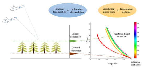
1. Introduction
2. Model-Based Inversion Algorithm
2.1. RVoG Model and Three-Stage Inversion Process
2.1.1. RVoG Model
2.1.2. Three-Stage Inversion Process
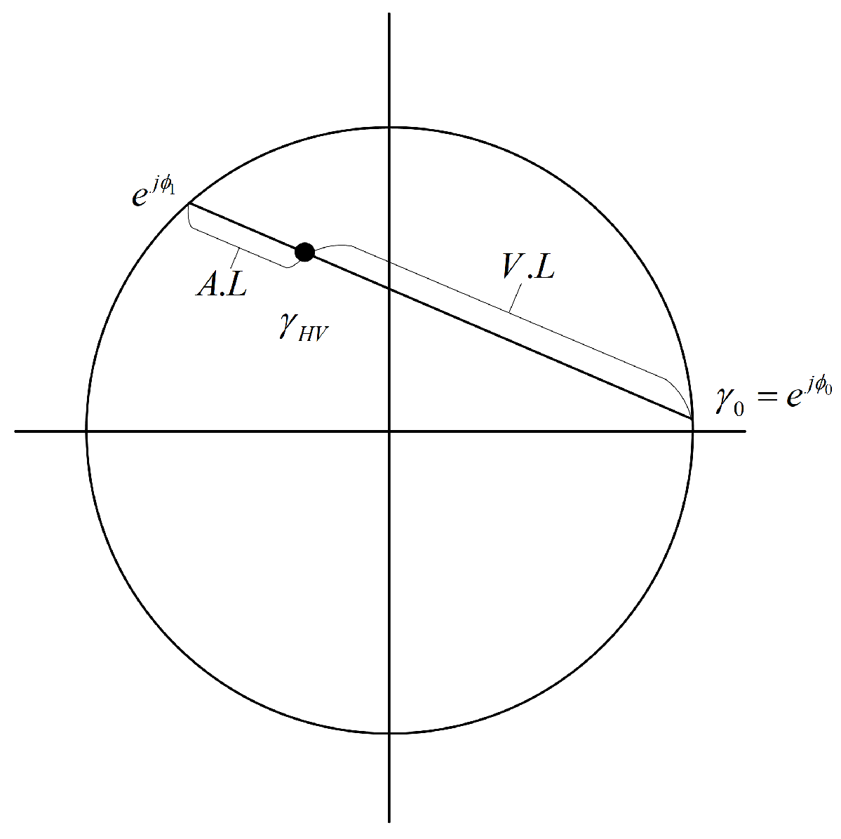
- Least squares line fit. Since Equation (5) indicates that coherence values in different polarization states lie along a straight line in CUC, the first stage is to find the best-fit line of interferometric coherence values in different polarization modes, such as HH, VV, HH-VV, HH+VV, and HV.
- Ground phase removal. In the second stage, ground phase must be determined and removed from the coherence. The phases of two intersection points of the straight line and the CUC are the candidates of ground phase. Generally, the relative location of coherence values in different polarization states along the best-fit line arranges according to Figure 1, which becomes one criterion for distinguishing the real ground phase.
- Height and extinction estimation. The pre-calculate look up table (LUT) of volume-only coherence is employed to estimate vegetation height and mean extinction in last stage. The parameters are determined by minimizing the distance between the calculated volume coherences and the observed volume coherence.
2.2. RVoG-vtd Model and Four-Stage Inversion Algorithm
2.2.1. RVoG-vtd Model
2.2.2. Four-Stage Inversion Algorithm
- Least squares line fit.
- Ground phase removal.
- Extinction estimation.
- Volume height and temporal decorrelation estimation.
2.3. GRVoG-vtd Model and a Novel Four-Stage Inversion Algorithm
2.3.1. GRVoG-vtd Model
2.3.2. A Novel Four-Stage Inversion Algorithm
- Generate the coherence in different polarization states and fit the least square line in the CUC.
- Choose the ground underlying phase from the two intersection points between the best fitted line and CUC. Calculate the volume coherence by removing the ground phase and projecting the farthest coherence from the ground coherence point to the fitted line.
- Classify sparse savannas and dense forest by the amplitude of the volume coherence using EM algorithm. Determine the constant parameter by calculating the mean value of the amplitude in sparse savanna region.
- Estimate the vegetation height and mean extinction based on the pre-calculate LUT of GRVoG-vtd model by minimizing the generalized distance between calculated volume coherences and the observed volume coherence.
2.4. Analysis of Models and Corresponding Algorithms
3. Results
3.1. Study Area
3.2. Data Set
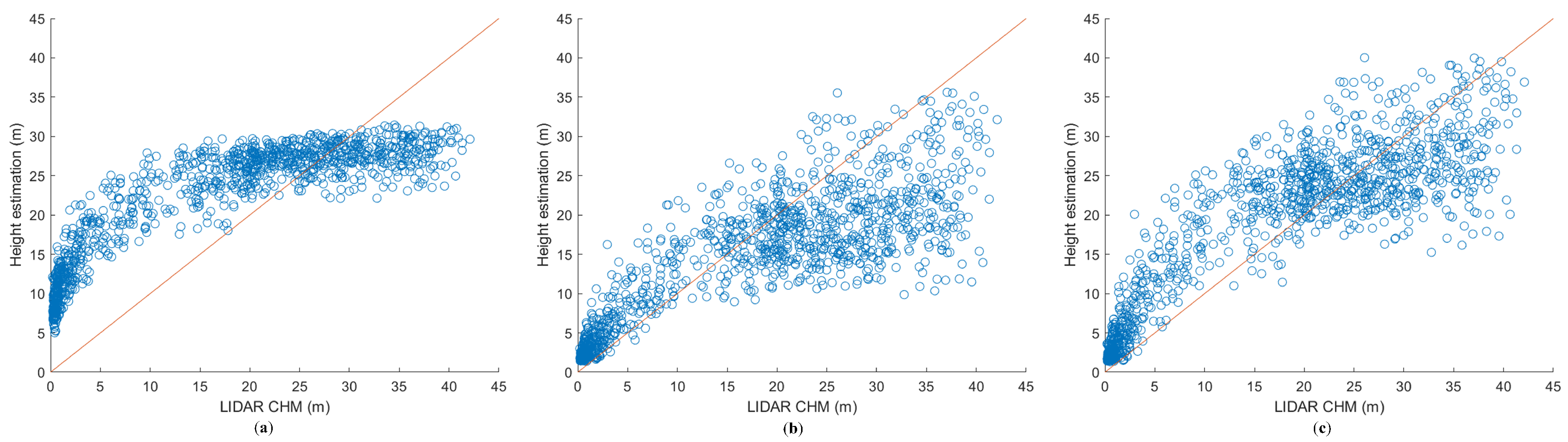
3.3. Experimental Results
4. Discussion
4.1. Analysis of Inversion Error
4.2. Discussions of Inversion Results
5. Conclusions
Author Contributions
Funding
Data Availability Statement
Acknowledgments
Conflicts of Interest
Abbreviations
| PolInSAR | Polarimetric interferometric synthetic aperture radar |
| LiDAR | Light detection and ranging |
| RVoG | Random volume over ground model |
| RVoG-vtd | Random volume over ground model with volumetric temporal decorrelation |
| GRVoG-vtd | Generalized RVoG-vtd |
| EM | Expectation-Maximum |
| DLR | German Aerospace Center |
| CUC | Complex unit circle |
| LUT | Look up table |
| GMM | Gaussian mixture model |
| RMSE | Root of mean square error |
Appendix A. The Derivation of the GRVoG Model Function
References
- Cloude, S.R.; Papathanassiou, K.P. Polarimetric optimisation in radar interferometry. Electron. Lett. 1997, 33, 1176–1178. [Google Scholar] [CrossRef]
- Papathanassiou, K.P.; Cloude, S.R. Single-baseline polarimetric SAR interferometry. IEEE Trans. Geosci. Remote Sens. 2001, 39, 2352–2363. [Google Scholar] [CrossRef]
- Cloude, S.R.; Papathanassiou, K.P. Polarimetric SAR Interferometry. IEEE Trans. Geosci. Remote Sens. 1998, 36, 1551–1565. [Google Scholar] [CrossRef]
- Yamada, H.; Sato, K.; Yamaguchi, Y.; Boerner, W.M. Interferometric phase and coherence of forest estimated by ESPRIT-based polarimetric SAR interferometry. In Proceedings of the IEEE International Geoscience and Remote Sensing Symposium, Toronto, ON, Canada, 24–28 June 2002. [Google Scholar]
- Ballester-Berman, J.D.; Lopez-Sanchez, J.M. Applying the Freeman–Durden Decomposition Concept to Polarimetric SAR Interferometry. IEEE Trans. Geosci. Remote Sens. 2009, 48, 466–479. [Google Scholar] [CrossRef]
- Aghababaee, H.; Sahebi, M.R. Model-Based Target Scattering Decomposition of Polarimetric SAR Tomography. IEEE Trans. Geosci. Remote Sens. 2018, 56, 972–983. [Google Scholar] [CrossRef]
- Treuhaft, R.N.; Madsen, S.N.; Moghaddam, M.; Van Zyl, J.J. Vegetation characteristics and underlying topography from interferometric radar. Radio Sci. 1996, 31, 1449–1485. [Google Scholar] [CrossRef]
- Treuhaft, R.N.; Siqueira, P.R. Vertical structure of vegetated land surfaces from interferometric and polarimetric radar. Radio Sci. 2016, 35, 141–177. [Google Scholar] [CrossRef]
- Lu, H.; Suo, Z.; Guo, R.; Bao, Z. S-RVoG model for forest parameters inversion over underlying topography. Electron. Lett. 2013, 49, 618–619. [Google Scholar] [CrossRef]
- Sun, X.; Wang, B.; Xiang, M.; Fu, X.; Li, Y. S-RVoG Model Inversion Based on Time-Frequency Optimization for P-Band Polarimetric SAR Interferometry. Remote Sens. 2019, 11, 1033. [Google Scholar] [CrossRef]
- Sun, X.; Wang, B.; Xiang, M.; Jiang, S.; Fu, X. Forest Height Estimation Based on Constrained Gaussian Vertical Backscatter Model Using Multi-Baseline P-Band Pol-InSAR Data. Remote Sens. 2018, 11, 42. [Google Scholar] [CrossRef]
- Wang, X.; Xu, F. A PolinSAR Inversion Error Model on Polarimetric System Parameters for Forest Height Mapping. IEEE Trans. Geosci. Remote Sens. 2019, 57, 5669–5685. [Google Scholar] [CrossRef]
- Bryan, R.; Michael, D.; Marco, L. Uncertainties in Forest Canopy Height Estimation From Polarimetric Interferometric SAR Data. IEEE J. Select. Top. Appli. Earth Observat. Remote Sens. 2018, 11, 1–14. [Google Scholar]
- Cloude, S.R.; Papathanassiou, K.P. Three-stage inversion process for polarimetric SAR interferometry. IEE Proc. Radar Sonar Navigat. 2003, 150, 125–134. [Google Scholar] [CrossRef]
- Managhebi, T.; Maghsoudi, Y.; Zoej, M.J.V. A Volume Optimization Method to Improve the Three-Stage Inversion Algorithm for Forest Height Estimation Using PolInSAR Data. IIEEE Trans. Geosci. Remote Sens. Lett. 2018, 15, 1–5. [Google Scholar] [CrossRef]
- Ballester-Berman, J.D.; Vicente-Guijalba, F.; Lopez-Sanchez, J.M. A Simple RVoG Test for PolInSAR Data. IEEE J. Select. Top. Appl. Earth Observat. Remote Sens. 2017, 8, 1028–1040. [Google Scholar] [CrossRef]
- Ghasemi, N.; Tolpekin, V.A.; Stein, A. Estimating Tree Heights Using Multibaseline PolInSAR Data With Compensation for Temporal Decorrelation, Case Study: AfriSAR Campaign Data. IEEE J. Select. Top. Appl. Earth Observat. Remote Sens. 2018, 11, 3464–3477. [Google Scholar] [CrossRef]
- Brigot, G.; Simard, M.; Colin-Koeniguer, E.; Boulch, A. Retrieval of Forest Vertical Structure from PolInSAR Data by Machine Learning Using LIDAR-Derived Features. Remote Sens. 2019, 11, 381. [Google Scholar] [CrossRef]
- Sun, X.; Wang, B.; Xiang, M.; Zhou, L.; Jiang, S. Forest Height Estimation Based on P-Band Pol-InSAR Modeling and Multi-Baseline Inversion. Remote Sens. 2020, 12, 1319. [Google Scholar] [CrossRef]
- Kumar, P.; Krishna, A.P. InSAR-Based Tree Height Estimation of Hilly Forest Using Multitemporal Radarsat-1 and Sentinel-1 SAR Data. IEEE J. Select. Top. Appl. Earth Observat. Remote Sens. 2020, 12, 5147–5152. [Google Scholar] [CrossRef]
- Xie, Y.; Fu, H.; Zhu, J.; Wang, C.; Xie, Q. A LiDAR-Aided Multibaseline PolInSAR Method for Forest Height Estimation: With Emphasis on Dual-Baseline Selection. IEEE Geosci. Remote Sens. Lett. 2019, 17, 1–10. [Google Scholar] [CrossRef]
- Pourshamsi, M.; Garcia, M.; Lavalle, M.; Balzter, H. A Machine-Learning Approach to PolInSAR and LiDAR Data Fusion for Improved Tropical Forest Canopy Height Estimation Using NASA AfriSAR Campaign Data. IEEE J. Select. Top. Appl. Earth Observat. Remote Sens. 2018, 11, 3453–3463. [Google Scholar] [CrossRef]
- Hajnsek, I.; Kugler, F.; Lee, S.K.; Papathanassiou, K.P. Tropical-Forest-Parameter Estimation by Means of Pol-InSAR: The INDREX-II Campaign. IEEE Trans. Geosci. Remote Sens. 2009, 47, 481–493. [Google Scholar] [CrossRef]
- Zebker, H.A.; Villasenor, J. Decorrelation in interferometric radar echoes. IEEE Trans. Geosci. Remote Sens. 1992, 30, 950–959. [Google Scholar] [CrossRef]
- Lavalle, M.; Khun, K. Three-Baseline Approach to Forest Tree Height Estimation. In Proceedings of the Eusar European Conference on Synthetic Aperture Radar, Berlin, Germany, 3–5 June 2014. [Google Scholar]
- Lavalle, M. A Temporal Decorrelation Model for Polarimetric Radar Interferometers. IEEE Trans. Geosci. Remote Sens. 2012, 50, 2880–2888. [Google Scholar] [CrossRef]
- Simard, M.; Denbina, M. An Assessment of Temporal Decorrelation Compensation Methods for Forest Canopy Height Estimation Using Airborne L-Band Same-Day Repeat-Pass Polarimetric SAR Interferometry. IEEE J. Select. Top. Appl. Earth Observat. Remote Sens. 2018, 11, 95–111. [Google Scholar] [CrossRef]
- Tayebe, M.; Yasser, M.; Mohammad, V.Z. Four-Stage Inversion Algorithm for Forest Height Estimation Using Repeat Pass Polarimetric SAR Interferometry Data. Remote Sens. 2018, 10, 1174. [Google Scholar]
- Pardini, M.; Tello, M.; Cazcarra-Bes, V.; Papathanassiou, K.P.; Hajnsek, I. L- and P-Band 3-D SAR Reflectivity Profiles Versus Lidar Waveforms: The AfriSAR Case. IEEE J. Select. Top. Appl. Earth Observat. Remote Sens. 2018, 11, 3386–3401. [Google Scholar] [CrossRef]
- Ngo, Y.N.; Minh, D.H.T.; Moussawi, I.; Villard, L.; Toan, T.L. Afrisar-Tropisar: Forest Biomass Retrieval by P-Band Sar Tomography. In Proceedings of the IGARSS 2018 IEEE International Geoscience and Remote Sensing Symposium, Valencia, Spain, 22–27 July 2018. [Google Scholar]
- Moussawi, I.E.; Minh, D.H.T.; Baghdadi, N.; Abdallah, C.; Strauss, O. L-Band Uavsar Tomographic Imaging in Dense Forest: Afrisar Results. In Proceedings of the IGARSS 2018 IEEE International Geoscience and Remote Sensing Symposium, Valencia, Spain, 22–27 July 2018. [Google Scholar]
- Technical Assistance for the Development of Airborne SAR and Geophysical Measurements during the AfriSAR Experiment. Available online: https://earth.esa.int/eogateway/documents/20142/37627/AfriSAR-Final-Report.pdf (accessed on 24 December 2020).
- Kugler, F.; Lee, S.K.; Hajnsek, I.; Papathanassiou, K.P. Forest Height Estimation by Means of Pol-InSAR Data Inversion: The Role of the Vertical Wavenumber. IEEE Trans. Geosci. Remote Sens. 2015, 53, 5294–5311. [Google Scholar] [CrossRef]
- Lang, R.H. Electromagnetic backscattering from a sparse distribution of lossy dielectric scatterers. Radio Sci. 1981, 16, 15–30. [Google Scholar] [CrossRef]
- Ishimaru, A. Wave Propagation and Scattering in Random Media; Academic Press: New York, NY, USA, 1978. [Google Scholar]


| Model | Bias | RMSE | |
|---|---|---|---|
| RVoG | 4.8123 | 8.6904 | 0.8699 |
| RVoG-vtd | −2.8665 | 7.7168 | 0.8438 |
| GRVoG-vtd | 1.2764 | 6.2341 | 0.8783 |
| Model | RVoG | RVoG-vtd | GRVoG-vtd | |||
|---|---|---|---|---|---|---|
| RMSE | Bias | RMSE | Bias | RMSE | Bias | |
| Sparse Savanna | 10.66 | 10.28 | 3.56 | 2.60 | 5.20 | 3.94 |
| Low Forest | 5.40 | 2.20 | 8.32 | −5.62 | 5.78 | −1.03 |
| High Forest | 7.91 | −6.21 | 10.64 | −8.62 | 7.41 | −5.82 |
Publisher’s Note: MDPI stays neutral with regard to jurisdictional claims in published maps and institutional affiliations. |
© 2021 by the authors. Licensee MDPI, Basel, Switzerland. This article is an open access article distributed under the terms and conditions of the Creative Commons Attribution (CC BY) license (http://creativecommons.org/licenses/by/4.0/).
Share and Cite
Xing, C.; Zhang, T.; Wang, H.; Zeng, L.; Yin, J.; Yang, J. A Novel Four-Stage Method for Vegetation Height Estimation with Repeat-Pass PolInSAR Data via Temporal Decorrelation Adaptive Estimation and Distance Transformation. Remote Sens. 2021, 13, 213. https://doi.org/10.3390/rs13020213
Xing C, Zhang T, Wang H, Zeng L, Yin J, Yang J. A Novel Four-Stage Method for Vegetation Height Estimation with Repeat-Pass PolInSAR Data via Temporal Decorrelation Adaptive Estimation and Distance Transformation. Remote Sensing. 2021; 13(2):213. https://doi.org/10.3390/rs13020213
Chicago/Turabian StyleXing, Cheng, Tao Zhang, Hongmiao Wang, Liang Zeng, Junjun Yin, and Jian Yang. 2021. "A Novel Four-Stage Method for Vegetation Height Estimation with Repeat-Pass PolInSAR Data via Temporal Decorrelation Adaptive Estimation and Distance Transformation" Remote Sensing 13, no. 2: 213. https://doi.org/10.3390/rs13020213
APA StyleXing, C., Zhang, T., Wang, H., Zeng, L., Yin, J., & Yang, J. (2021). A Novel Four-Stage Method for Vegetation Height Estimation with Repeat-Pass PolInSAR Data via Temporal Decorrelation Adaptive Estimation and Distance Transformation. Remote Sensing, 13(2), 213. https://doi.org/10.3390/rs13020213