Abstract
Soil organic carbon (SOC) is a key property for evaluating soil quality. SOC is thus an important parameter of agricultural soils and needs to be regularly monitored. The aim of this study is to explore the potential of synthetic aperture radar (SAR) satellite imagery (Sentinel-1), optical satellite imagery (Sentinel-2), and digital elevation model (DEM) data to estimate the SOC content under different land use types. The extreme gradient boosting (XGboost) algorithm was used to predict the SOC content and evaluate the importance of feature variables under different land use types. For this purpose, 290 topsoil samples were collected and 49 features were derived from remote sensing images and DEM. Feature selection was carried out to prevent data redundancy. Coefficient of determination (R2), mean absolute error (MAE), mean squared error (MSE), percent root mean squared error (%RMSE), ratio of performance to interquartile range (RPIQ), and corrected akaike information criterion (AICc) were employed for evaluating model performance. The results showed that Sentinel-1 and Sentinel-2 data were both important for the prediction of SOC and the prediction accuracy of the model differed with land use types. Among them, the prediction accuracy of this model is the best for orchard (R2 = 0.86 and MSE = 0.004%), good for dry land (R2 = 0.74 and MSE = 0.008%) and paddy field (R2 = 0.66 and MSE = 0.009%). The prediction model of SOC content is effective and can provide support for the application of remote sensing data to soil property monitoring.
1. Introduction
Terrestrial ecosystem is an important carbon pool, most of which is stored in soil [1]. There is an exchange of carbon dioxide (CO2) between the atmosphere and soil, which leads to the sequestration or emission of CO2 by soil [2]. Moreover, soil organic carbon (SOC) is closely related to soil fertility, plant growth, conservation of soil and water, aggregate stability, and soil nutrient cycling capability [3]. Both natural factors (soil type, climate, and topography) and human activities (land use and farming practices) affect the content of SOC [4]. However, the carbon storage in soil is limited and the carbon content in the soil will gradually reach saturation with the increase of SOC storage [5]. Therefore, it is necessary to monitor the content of SOC. However, the traditional method of measuring sample points is time-consuming and costly [6], and thus is not suitable for large-scale monitoring. In order to solve these problems, scholars gradually began to explore the use of robust and cost-effective approaches to predict SOC content.
In recent studies, scholars have mostly used laboratory-based soil reflectance spectroscopy to predict SOC content [7,8,9,10,11,12,13]. They selected several spectral bands (visible, mid-infrared, near-infrared, and short-wave infrared spectroscopy) for prediction. Although these methods have a good prediction accuracy, with coefficient of determination (R2) approximately greater than 0.83, the laboratory spectrum has some limitations; that is, it can only provide spectral data at the point scale, but not at the landscape scale [14]. The remote sensing data are easy to obtain, covering a wide range, and can be used for ground monitoring throughout the year. Therefore, it is necessary to explore the contribution of remote sensing data to SOC prediction. There have been some studies on SOC prediction based on remote sensing data that achieved good prediction results, especially optical data (e.g., Sentinel-2 [15,16,17,18,19,20,21], Landsat [22,23,24,25,26,27,28], and MODIS satellite data [29,30,31]); their bands cover from visible to short-wave infrared, providing more information. However, the application of optical data is susceptible to weather conditions, especially in the Sichuan Basin where clouds occur most frequently [32], so the available optical data are very limited. Moreover, soil surface conditions (e.g., vegetation coverage, debris, soil moisture, and soil roughness) also affect SOC prediction [19].
Synthetic aperture radar (SAR) technology has the advantages of all-weather, day and night imaging [33]. Therefore, the spectral range from remote sensing used for SOC prediction is not limited to the visible and infrared; radar can and have also be used [34,35,36]. Recent studies have found that multitemporal SAR data could capture the soil–vegetation relationship to predict soil chemical properties, and its ability depends on capturing vegetation characteristics from remote sensing images that indicate variation of soil properties [37]. Yang and Guo [38] reported fluctuation correlations between the backscattering coefficients of multitemporal Sentinel-1 images and SOC. SAR data have broad application prospects for the prediction of soil properties [33,38], but its application in predicting SOC is still limited and rarely reported in the literature due to its complexity, diversity, and availability (e.g., the preprocessing of SAR data is more complicated and has less information than optical data) [36,39]. The newly released Sentinel satellites developed by the European Space Agency (ESA) have the advantages of short revisit time (Sentinel-1: 6 days; Sentinel-2: 5 days), high spatial resolution (Sentinel-1: 5–20 m; Sentinel-2: 10–60 m), free download, and high-quality physical calibration data. They can provide a large amount of free optical and SAR remote sensing data with high spatial resolution for SOC prediction.
The hilly areas in the Sichuan Basin have diverse land use types, with small and scattered plots. Complex ground conditions add uncertainties to the SOC prediction with remote sensing data. There have been many studies on the influence of land use change on SOC content, but fewer on the prediction accuracy of SOC content under different land use types. Studies have shown that land use has a significant effect on the SOC content [40,41]. Land use effects on SOC are related to the land use conversion that has led to the exposure of soils and the rapid decomposition of SOC [42], so the prediction accuracy of SOC content may be affected by land use types. Zhou et al. [36], Zhang et al. [43], and Paul et al. [44] used land use type as a variable to predict SOC content, but the results showed that it did not contribute much to the model. In recent studies, remote sensing data were used to predict SOC content based on multiple land use types, while the results showed that the accuracy of SOC prediction using satellite remote sensing data was lower than that using airborne remote sensing and laboratory reflectance spectra data [19,45]. Therefore, it is possible to improve the prediction accuracy of SOC based on satellite remote sensing data under a single land use type.
The main purposes of this study were to (1) explore the joint application of radar and optical remote sensing in SOC prediction and (2) compare the prediction accuracy of SOC under different land use types. The SOC content was predicted by considering the relationship between SOC and environmental auxiliary variables in the vegetation-covered area. Specifically, SAR satellite imagery (Sentinel-1), optical satellite imagery (Sentinel-2), and digital elevation model (DEM) data were used as input variables. The extreme gradient boosting (XGboost) algorithm has been used to predict SOC with good prediction results [17,22,29,30]. Therefore, we used XGboost to build prediction models of SOC content under different land use types and analyze the importance of feature variables. The results of this study would contribute to the application of remote sensing data for the effective monitoring of SOC content.
2. Materials and Methods
2.1. Study Area
The study area is located in Ganning Town, Wanzhou District, Chongqing (108°13′10″–108°17′40″E, 30°39′1″–30°41′30″N) and covers 1800 hectares (Figure 1). The soil developed from purple shale is characterized by 0.5 to 0.8 m depth, relatively light texture, and susceptibility to water erosion [46,47]. The pH value of the soil varies from 4.63 to 8.43, and acid soils mainly dominate the study area. The landform type is tectonic denudation hills in eastern Sichuan. The altitude ranges from 248 to 657 m, with an average of 433 m. The slope is between 0 and 79° and the average is 13°. The study site is located in subtropical monsoon humid area, with annual average temperature of 17 °C and annual average rainfall of 1293.3 mm.
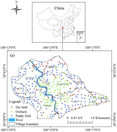
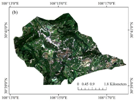
Figure 1.
(a) Location of study area and distribution of soil sample points and (b) RGB (red: 665 nm; green: 560 nm; blue: 490 nm) images acquired by optical satellite imagery (Sentinel-2) sensor.
The main land use types in the study area are orchard, dry land, and paddy field, which account for 12%, 13%, and 30% of the area, respectively. Dry land is mainly planted with wheat (Triticum aestivum L.), corn (Zea mays Linn.), sweet potato (Ipomoea batatas (L.) Lam.), and peanut (Arachis hypogaea Linn.). Orchard grows blood oranges (Citrus sinensis (L.) Osbeck). Single cropping rice (Oryza sativa L.) is planted in paddy field; the growth period of rice in the study area is from April to September, and it is used for water storage in winter. The land use types in the study area are representative of southwestern China.
2.2. Sample Collection and Preparation
Soil sampling was conducted in March 2019. According to the requirements of soil sampling point layout in DZ/T 0295–2016 Specification of Land Quality Geochemical Assessment, 290 topsoil samples were arranged based on parcel of land and grid, and the sampling medium was 0–20 cm soil column on the surface (Figure 1). About 3–5 subsoil columns were collected within a radius of 10 m around the sampling points to form one sample, and the land use type and soil type of each subsampling point were basically the same. The original weight of the samples was generally more than 1.5 kg, which was stored in a special sample bag. Samples were air-dried at room temperature and passed through a 2 mm soil sieve before soil chemical analyses. After that, soil samples weighing 0.5 g were taken, then potassium dichromate–sulfuric acid solution was added, and it was heated on the electric heating plate for digestion. Soil organic carbon (percent of content) was determined by the redox volumetric method [48].
2.3. Data Acquisition and Processing
2.3.1. Sentinel-1 Images
Sentinel-1 satellite is an earth observation system in the Copernicus Program of ESA. It consists of two satellites and carries C-band synthetic aperture radar, which can provide continuous images and is not affected by the weather [49]. Six ground range detected (GRD) format images of Interferometric Wide Swath Mode (IW) from October 2018 to September 2019 were selected in this paper. Single temporal Sentinel-1 image contains less information, so we chose multitemporal Sentinel-1 images with a growth period (one year). All images were downloaded from Sentinel Scientific Data Center of ESA. Images are VH (vertical—horizontal) and VV (vertical—vertical) dual polarization, resulting in 12 images with a resolution of 20 m (Table 1). In this study, the Sentinel-1 data were preprocessed by SNAP 7.0, including calibration, thermal noise removal, multilooking, speckle filtering, and terrain correction. Finally, it was converted into VV and VH polarization in dB format without further conversion; the mean values of VV and VH at six time points are shown in Figure 2. The mean values of VV and VH differ with time and land use type, indicating that multitemporal Sentinel-1 data may be helpful for SOC prediction [38].

Table 1.
Sentinel-1 data set.
Figure 2.
The mean values of vertical—vertical (VV) (a) and vertical—horizontal (VH) (b) of SAR satellite imagery (Sentinel-1) at six time points; 1, 2, 3, 4, 5, and 6 in the abscissa represent the times, which are 26 October 2018, 7 March 2019, 6 May 2019, 5 July 2019, 22 August 2019, and 15 September 2019, respectively.
2.3.2. Sentinel-2 Images
Sentinel-2 image acquired on 12 August 2019 was also from the official website of ESA. This is because only this image has no cloud cover in the study area, and its acquisition time is close to the sampling time. The image is of L2A level, so it does not require atmospheric correction. The data of each band was resampled to 10 m resolution in SNAP 7.0. Ten bands (B2, B3, B4, B5, B6, B7, B8, B8a, B11, B12) with higher resolution were reserved, and the four soil radiometric indices and twenty vegetation radiometric indices were calculated on this basis (Appendix A: Table A1).
2.3.3. DEM and Land Use
The elevation, slope, and aspect data of the study area were extracted by ArcGIS 10.5, based on the 5 m resolution DEM data produced by the national surveying and mapping department that are available at https://www.webmap.cn/ (accessed on 30 June 2020). Land use data were derived from the 1:10,000 land use map in 2019, which can be obtained from the Ministry of Natural Resources of the People’s Republic of China, are available at http://www.mnr.gov.cn/ (accessed on 21 June 2020). This land use map came from the land use database of Wanzhou District, which was established in 2008 and is updated by the local Ministry of Natural Resources every year [50].
2.4. Statistical Analysis
One-way analysis of variance (ANOVA) and multiple comparisons (least significant difference test, LSD) were applied to analyze the differences in SOC content under different land use types. The confidence interval was 0.05. Pearson correlation was used to analyze the correlation between features and SOC content. These statistical analyses were performed with SPSS V. 25.
2.5. XGboost Algorithm
The extreme gradient boosting is an improved algorithm based on the gradient boosting decision tree (GBDT), which can run in parallel based on the constructed boosting tree [51]. The core of the algorithm is to optimize the value of the objective function. In order to prevent overfitting, XGboost not only adds a regularization term to the cost function to control the complexity of the model, but also uses shrinkage and column subsampling. Shrinkage means that a nonnegative factor less than 1 is used to scale the newly added score after each iteration of tree boosting. Column subsampling means that only the ratio of training data samples is used to determine the XGboost model [52]. In short, the prediction process is as follows: (1) the function of projecting a set of predictor variables into an output variable is estimated by minimizing the loss function. (2) The model uses this loss function to iteratively fit the regression tree model for the calibration data. (3) The predicted values of each iteration are combined and multiplied by the weight of regression tree model to obtain the final prediction results [31]. The XGboost model implemented in Python 3.7.4 was used in this study.
The feature selection of XGboost is to establish a model based on the initial feature set, test the performance of the feature in the model, and obtain the importance of the feature. The more a feature is used to make critical decisions on the boosting tree, the higher its score [53]. The algorithm calculates the importance of features by “gain”, “frequency”, and “coverage”. Gain is the main reference factor that determines the importance of branch features. Frequency is a simplification of gain and is measured by the number of times the feature appears in all construction trees. Coverage is the relative value of feature observation [54]. The importance of features in this study is determined by gain.
For a single tree T, if J is selected as the split variable on this tree, the sum of mean square errors on all branch nodes t is calculated [54]. For example, the importance of feature j on the tree is as follows:
where it2 is the improvement of squared error of a node t, and υt is the feature associated with node t. By summing and averaging the importance of feature j on each tree, the final importance of the forest with M trees can be obtained:
2.6. Assessing Model Performance
The prediction models under total area, orchard, dry land, and paddy field were compared to explore the difference in SOC prediction under different land use types. All models were based on mixed signal including both soil and vegetation. In the previous experiment, we found that the sole use of DEM, Sentinel-1, and Sentinel-2 were relatively poor in predicting SOC (Appendix A: Table A2), so we explored their combined effect. Four models with different input combinations were built from the attribute values (corresponding to soil data points) of the predictor variables generated in Section 2.3; namely, Model A: DEM and Sentinel-1-derived features, Model B: DEM and Sentinel-2-derived features, Model C: DEM and Sentinel-1/-2-derived features, and Model D: the selected features from DEM, Sentinel-1, and Sentinel-2. We designed a set of candidate combinations to adjust the value of learning rate (0.01, 0.05, 0.1), maximum depth of tree (2, 20), minimum child weight (0, 20), and regression lambda (0, 20), number of boost round (0, 1000) for each model under total area, orchard, dry land, and paddy field. We randomly selected 80% of the sample points of each land use type as the calibration data set and the remaining 20% as the validation data set [31]. The optimal parameters for the models were calculated based on the calibration set (Appendix A: Table A3). The validation data set was employed to evaluate model performance under total area, orchard, dry land, and paddy field (Appendix A: Table A4).
Six common performance indicators including: R2, mean absolute error (MAE), mean squared error (MSE), percent root mean square error (%RMSE), ratio of performance to interquartile range (RPIQ), and corrected akaike information criterion (AICc) were used to assess model performance under different land use types. R2 varies between 0 and 1, which indicates the closeness between the observed value and the fitting regression line or the variance ratio explained by independent predictors [17]. The model has great fitting degree and stability when R2 closes to 1. The smaller the MSE and MAE, the better the predictive ability and robustness of the model [55]. %RMSE is dimensionless, and the accuracy of the model is excellent when %RMSE < 10%, good if 10% ≤ %RMSE < 20%, fair if 20% ≤ %RMSE < 30%, and poor if %RMSE ≥ 30% [56]. Generally, a larger value of RPIQ indicates better model performance. The model with the lowest AICc is the most concise.
where m is the number of samples, yi is the true value, ŷi is the predicted value, is the average value of yi, IQ is the interquartile range (IQ = Q3 − Q1) of the true value, Q1 and Q3 denote the first and third quartiles, respectively, SS is the sum squared residual, and K is the number of features.
3. Results
3.1. Statistical Analysis of SOC
The descriptive statistics of SOC under total area, orchard, dry land, and paddy field are shown in Table 2. The mean value of SOC content in total area was relatively high. For different land use types, the average contents of SOC in orchard and paddy field were higher. This is because the time of soil sampling in orchard is in the fertilization period after blood orange picking (mainly organic fertilizer), whereas paddy field is conducive to the accumulation of SOC in the process of cultivation and fertilization [57]. The mean, minimum, and maximum values of SOC in dry land were all low. The reason is that the physical protection of organic matter in dry land is weak [58], farming periodically decomposes large aggregates, exposing the previously protected organic matter in large soil aggregates [59], which is not conducive to the accumulation of SOC.
Table 2.
The statistics of SOC (%) under total area, orchard, dry land, and paddy field.
According to one-way ANOVA and multiple comparisons, the orchard, dry land, and paddy field had significant difference in SOC content (p < 0.05). The results showed that SOC content was affected by land use types to some extent [60]. Pearson correlation analysis showed that all the features had significant or slight correlation with SOC content under different land use types. In orchard, SOC content had significant correlation with Sentinel-2 data set and DEM data set. SOC content in dry land was only strongly correlated with some features of Sentinel-2 data set. In the paddy field, the three data sets all had features that had a significant correlation with the SOC content. See Table A5 (Appendix A) for details.
3.2. Analysis of SOC Prediction Results
3.2.1. Feature Selection and Model Evaluation
In order to explore the role of different remote sensing data in SOC prediction, we used twelve Sentinel-1-derived predictors, thirty-four Sentinel-2-derived predictors, and three DEM-derived predictors (Appendix A: Table A5) to establish the following three models: Model A, Model B, and Model C (Table 3). From the prediction results, the prediction accuracy of SOC under total area was significantly lower than that under three land use types. Among Model A, Model B, and Model C, the prediction accuracy of Model B was higher than that of Model A; it showed that Sentinel-1 and DEM-derived predictors were not as effective as Sentinel-2 and DEM-derived predictors in SOC prediction. However, Model C had the highest R2 (0.35, 0.85, 0.67, and 0.66, respectively) and the smallest error (e.g., MAE was 0.143%, 0.053%, 0.066%, and 0.077%, respectively). It showed that prediction model could get higher accuracy under the synergistic effect of Sentinel-1, Sentinel-2, and DEM data.
Table 3.
Prediction accuracy of models with different input combinations under total area, orchard, dry land, and paddy field.
Although Model C had the best prediction accuracy, the value of AICc was too large. For the sake of reducing the complexity of XGboost model and preventing data redundancy, feature selection was done for each land use type and total area. Firstly, the collected 49 features were input to the models. Then, the feature importance ranking was output. Finally, according to this ranking, features were added to the model from high to low. We selected those features that produced maximal R2. For example, the relationship between the number of features and R2 under total area is shown in Figure 3a. When the number of features was 39, R2 reached the largest value and then declined. The addition of following features with lower importance reduced model predictive accuracy. Therefore, the top 39 features with higher feature importance were selected as the input variables of the model under the total area. Similarly, the numbers of features were 25 for orchard, 26 for dry land, and 43 for paddy field (Figure 3). In this case, Model D was established by the selected features (detailed features and their importance scores are given in Section 3.2.2).
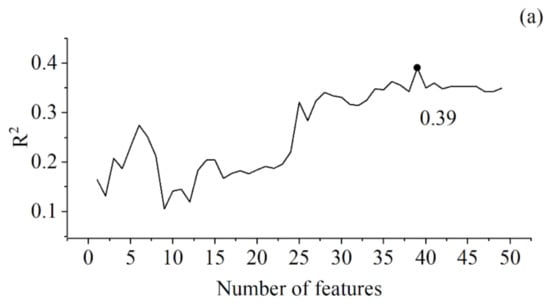
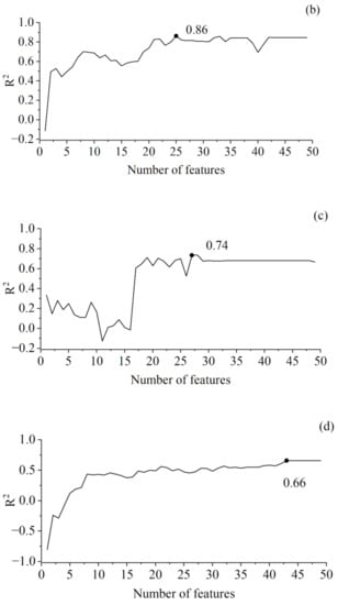
Figure 3.
Coefficient of determination (R2) of extreme gradient boosting (XGboost) changes with the selected features from digital elevation model (DEM), Sentinel-1, and Sentinel-2 under total area (a), orchard (b), dry land (c), and paddy field (d).
The prediction accuracy of Model D under different land use types and total area is shown in Table 4. The AICc of Model D was lower than that of Model C and the value of R2 did not decrease, indicating that feature selection was effective in reducing complexity of the model. For total area, the prediction accuracy was still lower than others after feature selection. However, for each land use type (Figure 4), the %RMSE in orchard, dry land, and paddy field was 7.87%, 13.11%, and 10.57%, respectively, showing that the model was excellent for orchard and good for dry land and paddy field. In addition, orchard had the highest R2 and lowest MAE and MSE, which further proves that the model had excellent prediction accuracy under this land use type. In dry land, R2, MAE, and MSE were 0.74, 0.057%, and 0.008%, respectively. Although the prediction result was not as good as that in orchard, it still showed that this model had good prediction accuracy in dry land. The value of %RMSE indicated that the prediction result of paddy field was as good as that of dry land, but the R2 of paddy field was lower than that of dry land, and MAE and MSE were higher than that of dry land, so there was a certain difference between paddy field and dry land. Although the prediction accuracy of paddy field was worse than that of orchard and dry land, the model of paddy field had better performance (RPIQ = 2.54). Comparing the prediction accuracy of the three models, it can be found that there were significant differences in the prediction accuracy of SOC for different land use types. Based on Model D, the map of SOC is presented in Figure 5.
Table 4.
Prediction accuracy of Model D with the selected features from DEM, Sentinel-1, and Sentinel-2 under total area, orchard, dry land, and paddy field.
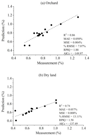
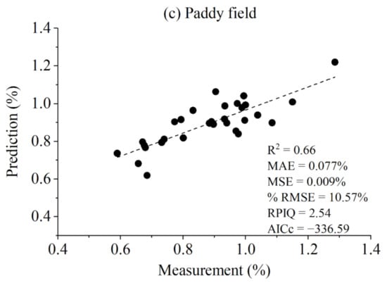
Figure 4.
Comparison of the measured and predicted soil organic carbon (SOC) (%) by Model D with the selected features from DEM, Sentinel-1, and Sentinel-2 under orchard (a), dry land (b), and paddy field (c).
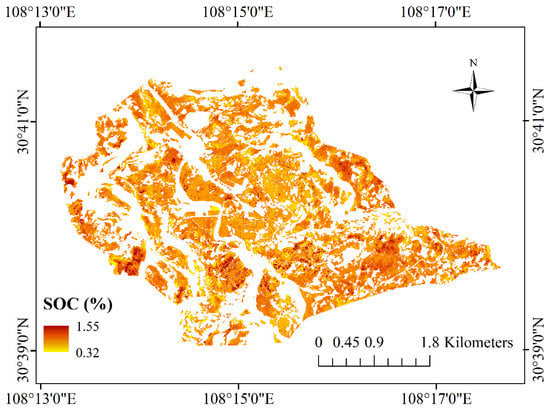
Figure 5.
Spatial distribution of SOC content based on Model D with the selected features from DEM, Sentinel-1, and Sentinel-2.
3.2.2. Importance of Predictor Variables
The feature importance score under orchard, dry land, and paddy field are shown in Figure 6. In orchard, the VV_5 (0.03) had the highest importance score, followed by CI (0.02), and BI2 (0.02) with similar scores. In dry land, BI2 (0.23), TSAVI (0.19), B8 (0.17), and MSAVI2 (0.15) of the Sentinel-2 data set were the most important. In paddy field, the B11 (0.09) band of the Sentinel-2 data set contributed the most. VV_5 (0.09) and VH_1 (0.08) of the Sentinel-1 data set also had a great contribution. For terrain indicators, only aspect (0.06) was slightly more important in paddy field, and it had little contribution to the other land use types.
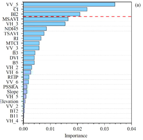
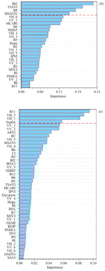
Figure 6.
Feature importance based on Model D with the selected features from DEM, Sentinel-1, and Sentinel-2 under orchard (a), dry land (b), and paddy field (c). VV_1 to VV_6 are the backscatter coefficients of VV polarization of six Sentinel-1 images, respectively (Table 1); VH_1 to VH_6 are the backscatter coefficients of VH polarization of six Sentinel-1 images, respectively (Table 1); other abbreviations are soil radiometric indices and vegetation radiometric indices of Sentinel-2 image (the meanings of these indices can be found in Appendix A: Table A1); the relative importance of the features above the red dotted line is greater than 60%.
4. Discussion
4.1. Performance of Prediction Models under Orchard, Dry Land, and Paddy Field
The results of Table 3 show that neither SAR data nor optical data alone can be used to make effective SOC prediction, and only the combination of the two can play a more comprehensive role. The usefulness of Sentinel-1 radar data in predicting SOC is proved [33]. Radar data can make up for the application defect of optical data in the hilly area of southwest China; that is, it can provide ground information in cloudy weather. Compared with existing studies, the results of SOC prediction based on multisource remote sensing data in this study are better than those based on single Sentinel-2 images (R2 = 0.56) [16] or Landsat images (R2 = 0.55) [25]. In addition, the application of high-resolution satellite images is also helpful for improving the prediction accuracy of SOC. The highest resolution of this image can reach 10 m, while Mahmoudzadeh et al. [23] and Hengl et al. [29] have reported general results by using Landsat-5 satellite data (30 m) and MODIS satellite data (250 m), respectively (R2 is about 0.5).
The effects of different land use types on the prediction of SOC content were explored. We found that the prediction accuracy under orchard, dry land, and paddy field was significantly higher than that under total area, and there were significant differences in the prediction accuracy among the three land use types (orchard > dry land > paddy field) (Table 4), which indicates that land use types have certain influence on the prediction accuracy of SOC content [12,61]. The reasons for this difference may be that: (1) the large area of orchard in the study area and the relatively uniform vegetation cover (blood orange) avoids the error of SAR data intensity value and optical data spectral information caused by the complex ground environment. (2) In the study area, the types of crop planted in dry land are diverse, which affects the feature variables, and the number of sample points was relatively insufficient, resulting in lower prediction accuracy than orchard. (3) In paddy field, soil moisture has a greater impact on SAR data, and due to the low spatial resolution and spectral resolution, as well as the effect of soil moisture [15], the performance of the short-wave infrared (SWIR) band was not good, resulting in poor prediction of SOC in paddy field. (4) Studies have shown that, in general, the prediction accuracy of the model will increase with the increase of coefficient of variation [62]. In this study, the coefficient of variation of dry land was higher than that of paddy field (Table 2), which may have had some influence on the prediction accuracy of SOC content.
It should be noted that there are still some limitations in using remote sensing data to predict SOC under a single land use type, which are mainly associated with the location-specific land use type, soil texture, and vegetation cover conditions. We used samples located in a small watershed for predictions, which may be regional (e.g., areas with the same land use type have similar vegetation and soil conditions). Further work is needed to prove whether it can be applied to other land use types and other larger areas. Furthermore, since we basically used all vegetation indices that currently exist, there is a correlation between the indices. Some excluded features (e.g., spectral bands of Sentinel-2) may have a greater correlation with SOC, but their effects have been replaced by other indices.
4.2. Variable Importance
The terrain controls the flow of solute, water, and sediment, which in turn affects the development of soil and the spatial distribution of soil properties [63]. Although terrain factors have a significant correlation with SOC content [64], the prediction ability of the model can be significantly improved by adding vegetation index and backscatter coefficient compared with those using only terrain variables [65]. On the one hand, the vegetation features have enough heterogeneity, and there is a strong interaction between vegetation features and soil properties [66]. On the other hand, the backscatter coefficient of SAR data is sensitive to the changes of surface conditions and soil moisture [67]. We found that there was a weak correlation between the polarization value of the Sentinel-1 image and the SOC content (Appendix A: Table A5), and Yang and Guo [38] have also proven that this correlation can be successfully used for SOC prediction. Therefore, both optical data (Sentinel-2) and radar data (Sentinel-1) can be used to build a predictive model of SOC content. In this study, the aspect made an important contribution to paddy field, and the other terrain variables data had a lower contribution than Sentinel-1 and Sentinel-2 data sets in orchard and dry land. Taghizadeh-Mehrjardi et al. [17] also found that Sentinel-2 bands have a greater correlation with SOC content than elevation while Zhou et al. [33] concluded that terrain variables are more important than Sentinel data in a study area with plains and plateaus. The difference may be because the range of altitude changes in this study was relatively small.
Due to the differences in the ground conditions of the three land use types, the contributions of remote sensing data in these models were different. In orchard, VV_5 had the highest score (Figure 6a); this is because the time of VV_5 (22 August 2019) was after summer pruning and weeding in orchard and it was the autumn shoot germination period of blood orange. At this time, the bare soil area in orchard increases, the contribution of ground scattering increases, and the contribution of canopy scattering decreases [68], which is more conducive to radar satellite reflecting the real situation of soil surface. VV polarization is mainly directly affected by the ground and canopy, whereas VH includes stem–ground double scattering and volume scattering [69] that has more interference information, so VV_5 is more important than VH_5 in orchard. The results in Figure 6a also indicate that CI and BI2 have made great contributions in orchard, due to soil color and soil brightness index having a high correlation with SOC content [19,70,71]. For dry land, BI2 also has a great influence on the prediction accuracy of SOC (Figure 6b). Because TSAVI and MSAVI2 have a significant correlation with SOC content (Appendix A: Table A5), and the close relationship between soil properties and vegetation coverage [66], TSAVI and MSAVI2 can effectively reflect the changes of SOC content. B8 band, which is the near-infrared band (NIR), ranks third in importance for dry land. Studies have shown that the near-infrared band has a good predictive effect on the carbon and nitrogen content in the soil [72]. In paddy field, B11 is the most important (Figure 6c). It may be that B11 band belongs to the short-wave infrared (SWIR) band, there is a strong correlation between reflectivity and SOC content in the SWIR region [15]. The importance of VH_5 (22 August 2019) and VH_1 (26 October 2018) follows B11. Firstly, VH is more sensitive to vegetation and VV is more sensitive to soil moisture [73], so VH is slightly more important than VV in paddy field. Secondly, since VH_5 is in the drainage time before rice harvest, it strengthens the contribution of stem–ground scattering in VH polarization; VH_1 is in the water storage period of paddy field, when the ground and canopy scattering of VV polarization is weakened and concentrated on the scattering of water surface, which is not conducive to reflecting SOC content in soil. It can be seen that in the three types of land use, both Sentinel-2 data set and Sentinel-1 data set have a great impact on the prediction of SOC.
5. Conclusions
This study presented and evaluated a method for predicting SOC content under different land use types based on remote sensing data. For this purpose, SAR satellite imagery (Sentinel-1), optical satellite imagery (Sentinel-2), and auxiliary DEM data were used for modeling. The influence of land use type on SOC prediction and the importance of optical and radar data under different land use types were analyzed. The overall prediction result of the model is better than some existing researches based on satellite remote sensing data [16,21,23,24,25,33], and is similar to the result of Taghizadeh-Mehrjardi et al. [17]. Among the three land use types, the prediction results of orchard (R2 = 0.86 and MSE = 0.004%) are better than dry land and paddy field. Both optical satellite imagery and radar satellite imagery have made important contributions to the prediction of SOC content. Although commonly used optical satellites, such as SPOT, Landsat 8 OLI, and Sentinel-2, have a large amount of information, it is difficult to obtain useful images because of the influence of cloud and fog. Whereas the radar satellites, such as GF-3, ALOS PALSAR, and Sentinel-1 SAR, have less information, but can obtain the continuous image. Therefore, it is necessary to combine the two images to study the real condition of the ground. Since the land use type has some influence on the prediction accuracy of SOC, in the future, analysis based on single land use type may improve the prediction results of SOC content.
Author Contributions
Methodology, H.W., H.L. and W.W.; resources, H.W. and H.L.; software, H.W.; supervision, H.L.; writing—original draft, H.W.; writing—review and editing, H.L., W.W. and X.Z. All authors have read and agreed to the published version of the manuscript.
Funding
This research received no external funding.
Institutional Review Board Statement
Not applicable.
Informed Consent Statement
Not applicable.
Data Availability Statement
Sentinel-1/-2, DEM, and land use data are publicly available online: Sentinel-1/2 images were acquired from the Copernicus Open Access Hub (https://scihub.copernicus.eu/ (accessed on 15 June 2020)), DEM were available at https://www.webmap.cn/ (accessed on 30 June 2020). Land use data were obtained from the Ministry of Natural Resources of the People’s Republic of China (http://www.mnr.gov.cn/ (accessed on 21 June 2020)); Soil sample data were obtained from Chongqing Key Laboratory of Land Quality Geological Survey and are available from the corresponding author with the permission of Chongqing Key Laboratory of Land Quality Geological Survey.
Acknowledgments
We thank the data support of Yu Li, Mingshu Yan, Lechao Yang, and Jiali Lei at Southeast Sichuan Geological Team of Chongqing Bureau of Geology and Mineral Exploration (Chongqing Key Laboratory of Land Quality Geological Survey).
Conflicts of Interest
The authors declare no conflict of interest.
Appendix A
Table A1.
Soil radiometric indices and vegetation radiometric indices.
Table A1.
Soil radiometric indices and vegetation radiometric indices.
| Type | Index | Formulation | References |
|---|---|---|---|
| Soil radiometric indices | Brightness Index (BI) | sqrt ((B42 + B32)/2) | [74] |
| Second Brightness Index (BI2) | sqrt ((B42 + B32 + B82)/3) | [74] | |
| Redness Index (RI) | B42/B33 | [75] | |
| Color Index (CI) | (B4 − B3)/(B4 + B3) | [75] | |
| Vegetation radiometric indices | Soil Adjusted Vegetation Index (SAVI) | (1 + L) × (B8 − B4)/(B8 + B4 + L) | [76] |
| Transformed Soil Adjusted Vegetation Index (TSAVI) | s × (B8 − s × B4 − a)/(s × B8 + B4 − a × s + X × (1 + s2)) | [77] | |
| Modified Soil Adjusted Vegetation Index (MSAVI) | (1 + M) × (B8 − B4)/(B8 + B4 + L) | [78] | |
| Second Modified Soil Adjusted Vegetation Index (MSAVI2) | (1/2) × (2 × B8 + 1 − sqrt ((2 × B8 + 1)2 − 8 × (B8 − B4))) | [79] | |
| Difference Vegetation Index (DVI) | B8 − B4 | [80] | |
| Ratio Vegetation Index (RVI) | B8/B4 | [81] | |
| Perpendicular Vegetation Index (PVI) | sin(b) × B8 − cos(b) × B4 | [82] | |
| Infrared Percentage Vegetation Index (IPVI) | B8/(B8 + B4) | [83] | |
| Weighted Difference Vegetation Index (WDVI) | (B8 − s × B4) | [84] | |
| Transformed Normalized Difference Vegetation Index (TNDVI) | Sqrt ((B8 − B4)/(B8 + B4) + 0.5) | [85] | |
| Green Normalized Difference Vegetation Index (GNDVI) | (B7 − B3)/(B7 + B3) | [86] | |
| Global Environmental Monitoring Index (GEMI) | eta × (1 − 0.25 × eta) − (B4 − 0.125)/(1 − B4) | [87] | |
| Atmospherically Resistant Vegetation Index (ARVI) | (B8 − rb)/(B8 + rb) | [88] | |
| Normalized Difference Index (NDI45) | (B5 − B4)/(B5 + B4) | [89] | |
| Meris Terrestrial Chlorophyll Index (MTCI) | (B6 − B5)/(B5 − B4) | [90] | |
| Modified Chlorophyll Absorption Ratio Index (MCARI) | [(B5 − B4) − 0.2 × (B5 − B3)] × (B5/B4) | [91] | |
| Red-Edge Inflection Point Index (REIP) | 705 + 35 × ((B4 + B7)/2 − B5)/(B6 − B5) | [92] | |
| Inverted Red-Edge Chlorophyll Index (IRECI) | (B7 − B4)/(B5/B6) | [93] | |
| Pigment Specific Simple Ratio algorithm (PSSRa) | B7/B4 | [94] | |
| Normalized Difference Vegetation Index (NDVI) | (B8 − B4)/(B8+ B4) | [95] |
L is a correction factor which ranges from 0 for very high vegetation cover to 1 for very low vegetation cover; a is the soil line intercept; s is the soil line slope; X is the adjustment factor to minimize soil noise; M = 1 − 2 × s × NDVI × WDVI; b is the angle between the soil line and the NIR axis, in degrees; eta = (2 × (B8A × B8A − B4 × B4) + 1.5 × B8A + 0.5 × B4)/(B8A + B4 + 0.5); rb = B4 − (B2 − B4). In this paper, L, a, s, X, and b are 0.5, 0.5, 0.5, 0.08, and 45, respectively.
Table A2.
The prediction accuracy (R2) of XGboost based on purely DEM, purely Sentinel-1, and purely Sentinel-2 under total area, orchard, dry land, and paddy field.
Table A2.
The prediction accuracy (R2) of XGboost based on purely DEM, purely Sentinel-1, and purely Sentinel-2 under total area, orchard, dry land, and paddy field.
| DEM | Sentinel-1 | Sentinel-2 | |
|---|---|---|---|
| Total area | 0.22 | 0.12 | 0.29 |
| orchard | 0.05 | 0.11 | 0.46 |
| dry land | 0.14 | 0.31 | 0.36 |
| paddy field | 0.10 | 0.04 | 0.46 |
Table A3.
The optimal values of parameters for models with different input combinations under total area, orchard, dry land, and paddy field.
Table A3.
The optimal values of parameters for models with different input combinations under total area, orchard, dry land, and paddy field.
| Land Use Type | Model | Eta | Max_Depth | Min_Child_Weight | Lambda | Num_Round |
|---|---|---|---|---|---|---|
| Total area | Model A | 0.05 | 3 | 2 | 1 | 64 |
| Model B | 0.05 | 3 | 3 | 1 | 70 | |
| Model C | 0.05 | 4 | 13 | 1 | 72 | |
| Model D | 0.05 | 4 | 13 | 1 | 72 | |
| Orchard | Model A | 0.05 | 7 | 1 | 1 | 999 |
| Model B | 0.05 | 1 | 2 | 1 | 894 | |
| Model C | 0.05 | 8 | 1 | 1 | 118 | |
| Model D | 0.05 | 8 | 1 | 1 | 118 | |
| Dry land | Model A | 0.05 | 2 | 3 | 1 | 54 |
| Model B | 0.05 | 3 | 5 | 1 | 70 | |
| Model C | 0.05 | 2 | 3 | 1 | 128 | |
| Model D | 0.05 | 2 | 3 | 1 | 128 | |
| Paddy field | Model A | 0.1 | 1 | 16 | 14 | 40 |
| Model B | 0.05 | 7 | 3 | 1 | 50 | |
| Model C | 0.1 | 6 | 1 | 1 | 41 | |
| Model D | 0.1 | 6 | 1 | 1 | 41 |
Model A, DEM and Sentinel-1-derived features; Model B, DEM and Sentinel-2-derived features data; Model C, DEM and Sentinel-1/-2-derived features; Model D, the selected features from DEM, Sentinel-1, and Sentinel-2; eta, learning rate; max_depth, maximum depth of tree; min_child_weight, minimum child weight; lambda, regression lambda; num_round, number of boost round.
Table A4.
The statistics of SOC (%) of calibration and validation data sets under total area, orchard, dry land, and paddy field.
Table A4.
The statistics of SOC (%) of calibration and validation data sets under total area, orchard, dry land, and paddy field.
| Calibration | Validation | |||||||||
|---|---|---|---|---|---|---|---|---|---|---|
| Land Use Type | Min | Max | Mean | SD | CV | Min | Max | Mean | SD | CV |
| Total area | 0.15 | 1.66 | 0.82 | 0.23 | 0.29 | 0.42 | 1.58 | 0.79 | 0.22 | 0.28 |
| Orchard | 0.40 | 1.32 | 0.75 | 0.19 | 0.26 | 0.55 | 1.28 | 0.80 | 0.18 | 0.22 |
| Dry land | 0.15 | 1.26 | 0.70 | 0.23 | 0.33 | 0.43 | 1.01 | 0.67 | 0.18 | 0.27 |
| Paddy field | 0.42 | 1.66 | 0.89 | 0.24 | 0.27 | 0.59 | 1.29 | 0.88 | 0.16 | 0.18 |
Min = minimum; Max = maximum; SD = standard deviation; CV = coefficient of variation.
Table A5.
The co-relationships between SOC (%) and environmental variables under orchard, dry land, and paddy field.
Table A5.
The co-relationships between SOC (%) and environmental variables under orchard, dry land, and paddy field.
| Type | Feature | Orchard | Dry Land | Paddy Field |
|---|---|---|---|---|
| Sentinel-1 | VH_1 | −0.11 | −0.14 | −0.01 |
| VV_1 | 0.01 | −0.12 | 0.06 | |
| VH_2 | −0.08 | 0.03 | −0.10 | |
| VV_2 | −0.11 | −0.13 | 0.06 | |
| VH_3 | −0.07 | −0.06 | −0.22 ** | |
| VV_3 | −0.10 | −0.05 | −0.18 * | |
| VH_4 | −0.16 | −0.21 | −0.11 | |
| VV_4 | −0.22 | −0.12 | −0.19 * | |
| VH_5 | −0.13 | 0.07 | −0.12 | |
| VV_5 | −0.14 | 0.03 | −0.12 | |
| VH_6 | −0.09 | −0.07 | 0.08 | |
| VV_6 | 0.00 | −0.12 | 0.08 | |
| Sentinel-2 | B2 | 0.26 * | 0.09 | −0.13 |
| B3 | 0.28 * | 0.05 | −0.15 | |
| B4 | 0.20 | 0.11 | −0.12 | |
| B5 | 0.26 * | 0.06 | −0.16 * | |
| B6 | 0.13 | −0.33 ** | −0.22 ** | |
| B7 | 0.11 | −0.33 ** | −0.09 | |
| B8 | 0.16 | −0.35 ** | −0.09 | |
| B8A | 0.11 | −0.34 ** | −0.09 | |
| B11 | 0.23 * | −0.10 | −0.33 ** | |
| B12 | 0.26 * | −0.01 | −0.24 ** | |
| BI | 0.25 * | 0.08 | −0.14 | |
| BI2 | 0.21 | −0.33 ** | −0.11 | |
| CI | 0.07 | 0.18 | −0.10 | |
| RI | −0.03 | 0.16 | −0.03 | |
| ARVI | −0.10 | −0.22 | 0.11 | |
| DVI | 0.06 | −0.35 ** | −0.02 | |
| GEMI | 0.00 | −0.34 ** | −0.01 | |
| GNDVI | −0.14 | −0.24 | 0.10 | |
| IPVI | −0.12 | −0.23 | 0.10 | |
| IRECI | −0.02 | −0.34 ** | −0.03 | |
| MCARI | 0.04 | −0.09 | 0.00 | |
| MSAVI | 0.02 | −0.34 ** | 0.01 | |
| MSAVI2 | 0.01 | −0.34 ** | 0.02 | |
| MTCI | −0.02 | −0.03 | −0.10 | |
| NDI45 | −0.09 | −0.13 | 0.09 | |
| NDVI | −0.12 | −0.23 | 0.10 | |
| PSSRA | −0.06 | −0.26 * | 0.10 | |
| PVI | 0.06 | −0.35 ** | −0.02 | |
| REIP | 0.00 | −0.14 | 0.25 ** | |
| RVI | −0.03 | −0.26 * | 0.08 | |
| SAVI | −0.01 | −0.33 ** | 0.02 | |
| TNDVI | −0.12 | −0.22 | 0.09 | |
| TSAVI | 0.17 | −0.31 ** | −0.14 | |
| WDVI | 0.02 | −0.34 ** | 0.00 | |
| DEM | Elevation | 0.01 | 0.19 | 0.21 * |
| Slope | −0.31 ** | −0.15 | −0.18 * | |
| Aspect | −0.04 | 0.05 | 0.06 |
*: Significance level at p < 0.05; **: Significance level at p < 0.01.
References
- Raich, J.W.; Potter, C.S.; Bhagawati, D. Interannual variability in global soil respiration, 1980–1994. Glob. Chang. Biol. 2002, 8, 800–812. [Google Scholar] [CrossRef]
- Karhu, K.; Auffret, M.D.; Dungait, J.A.; Hopkins, D.W.; Prosser, J.I.; Singh, B.K.; Subke, J.A.; Wookey, P.A.; Agren, G.I.; Sebastia, M.T.; et al. Temperature sensitivity of soil respiration rates enhanced by microbial community response. Nature 2014, 513, 81–84. [Google Scholar] [CrossRef]
- McBratney, A.B.; Stockmann, U.; Angers, D.A.; Minasny, B.; Field, D.J. Challenges for Soil Organic Carbon Research. In Soil Carbon; Hartemink, A.E., McSweeney, K., Eds.; Springer: Cham, Switzerland, 2014; pp. 3–16. [Google Scholar]
- Zhang, G.; Zheng, C.Y.; Wang, Y.; Li, Y.F.; Xin, Y. Soil organic carbon and microbial community structure exhibit different responses to three land use types in the North China Plain. Agric. Scand. Sect. B Soil Plant Sci. 2015, 65, 341–349. [Google Scholar] [CrossRef]
- Wang, S.Q.; Liu, J.Y.; Yu, G.R.; Pan, Y.Y.; Chen, Q.M.; Li, K.R.; Li, J.Y. Effects of land use change on the storage of soil organic carbon: A case study of the Qianyanzhou Forest Experimental Station in China. Clim. Chang. 2004, 67, 247–255. [Google Scholar]
- Aldana-Jague, E.; Heckrath, G.; Macdonald, A.; Van Wesemael, B.; Van Oost, K. UAS-based soil carbon mapping using VIS-NIR (480–1000 nm) multi-spectral imaging: Potential and limitations. Geoderma 2016, 275, 55–66. [Google Scholar] [CrossRef]
- Baldock, J.A.; Hawke, B.; Sanderman, J.; Macdonald, L.M. Predicting contents of carbon and its component fractions in Australian soils from diffuse reflectance mid-infrared spectra. Soil Res. 2013, 51, 577–583. [Google Scholar] [CrossRef]
- Lu, P.; Wang, L.; Niu, Z.; Li, L.; Zhang, W. Prediction of soil properties using laboratory VIS–NIR spectroscopy and Hyperion imagery. J. Geochem. Explor. 2013, 132, 26–33. [Google Scholar] [CrossRef]
- Liu, J.B.; Han, J.C.; Zhang, Y.; Wang, H.Y.; Kong, H.; Shi, L. Prediction of soil organic carbon with different parent materials development using visible-near infrared spectroscopy. Spectroc. Acta Pt. A Molec. Biomolec. Spectr. 2018, 204, 33–39. [Google Scholar] [CrossRef] [PubMed]
- Stevens, A.; Nocita, M.; Toth, G.; Montanarella, L.; van Wesemael, B. Prediction of Soil Organic Carbon at the European Scale by Visible and Near InfraRed Reflectance Spectroscopy. PLoS ONE 2013, 8, e66409. [Google Scholar] [CrossRef] [PubMed]
- Liu, L.F.; Ji, M.; Dong, Y.Y.; Zhang, R.C.; Buchroithner, M. Quantitative Retrieval of Organic Soil Properties from Visible Near-Infrared Shortwave Infrared (Vis-NIR-SWIR) Spectroscopy Using Fractal-Based Feature Extraction. Remote Sens. 2016, 8, 1035. [Google Scholar] [CrossRef]
- Zhang, Y.K.; Hartemink, A.E. Data fusion of vis-NIR and PXRF spectra to predict soil physical and chemical properties. Eur. J. Soil Sci. 2020, 71, 316–333. [Google Scholar] [CrossRef]
- Rossel, R.A.V.; Walvoort, D.J.J.; McBratney, A.B.; Janik, L.J.; Skjemstad, J.O. Visible, near infrared, mid infrared or combined diffuse reflectance spectroscopy for simultaneous assessment of various soil properties. Geoderma 2006, 131, 59–75. [Google Scholar] [CrossRef]
- Peng, Y.; Xiong, X.; Adhikari, K.; Knadel, M.; Grunwald, S.; Greve, M.H. Modeling Soil Organic Carbon at Regional Scale by Combining Multi-Spectral Images with Laboratory Spectra. PLoS ONE 2015, 10, e0142295. [Google Scholar] [CrossRef]
- Castaldi, A.; Chabrillat, S.; Don, A.; van Wesemael, B. Soil Organic Carbon Mapping Using LUCAS Topsoil Database and Sentinel-2 Data: An Approach to Reduce Soil Moisture and Crop Residue Effects. Remote Sens. 2019, 11, 2121. [Google Scholar] [CrossRef]
- Vaudour, E.; Gomez, C.; Fouad, Y.; Lagacherie, P. Sentinel-2 image capacities to predict common topsoil properties of temperate and Mediterranean agroecosystems. Remote Sens. Environ. 2019, 223, 21–33. [Google Scholar] [CrossRef]
- Taghizadeh-Mehrjardi, R.; Schmidt, K.; Amirian-Chakan, A.; Rentschler, T.; Zeraatpisheh, M.; Sarmadian, F.; Valavi, R.; Davatgar, N.; Behrens, T.; Scholten, T. Improving the Spatial Prediction of Soil Organic Carbon Content in Two Contrasting Climatic Regions by Stacking Machine Learning Models and Rescanning Covariate Space. Remote Sens. 2020, 12, 1095. [Google Scholar] [CrossRef]
- Castaldi, F.; Hueni, A.; Chabrillat, S.; Ward, K.; Buttafuoco, G.; Bomans, B.; Vreys, K.; Brell, M.; van Wesemael, B. Evaluating the capability of the Sentinel 2 data for soil organic carbon prediction in croplands. ISPRS J. Photogramm. Remote Sens. 2019, 147, 267–282. [Google Scholar] [CrossRef]
- Gholizadeh, A.; Zizala, D.; Saberioon, M.; Boruvka, L. Soil organic carbon and texture retrieving and mapping using proximal, airborne and Sentinel-2 spectral imaging. Remote Sens. Environ. 2018, 218, 89–103. [Google Scholar] [CrossRef]
- Zhou, T.; Geng, Y.; Ji, C.; Xu, X.; Wang, H.; Pan, J.; Bumberger, J.; Haase, D.; Lausch, A. Prediction of soil organic carbon and the C:N ratio on a national scale using machine learning and satellite data: A comparison between Sentinel-2, Sentinel-3 and Landsat-8 images. Sci. Total Environ. 2021, 755, 142661. [Google Scholar] [CrossRef]
- Vaudour, E.; Gomez, C.; Lagacherie, P.; Loiseau, T.; Baghdadi, N.; Urbina-Salazar, D.; Loubet, B.; Arrouays, D. Temporal mosaicking approaches of Sentinel-2 images for extending topsoil organic carbon content mapping in croplands. Int. J. Appl. Earth Obs. Geoinf. 2021, 96, 102277. [Google Scholar] [CrossRef]
- Ramcharan, A.; Hengl, T.; Nauman, T.; Brungard, C.; Waltman, S.; Wills, S.; Thompson, J. Soil Property and Class Maps of the Conterminous United States at 100-Meter Spatial Resolution. Soil Sci. Soc. Am. J. 2018, 82, 186–201. [Google Scholar] [CrossRef]
- Mahmoudzadeh, H.; Matinfar, H.R.; Taghizadeh-Mehrjardi, R.; Kerry, R. Spatial prediction of soil organic carbon using machine learning techniques in western Iran. Geoderma Reg. 2020, 21, e00260. [Google Scholar] [CrossRef]
- Emadi, M.; Taghizadeh-Mehrjardi, R.; Cherati, A.; Danesh, M.; Mosavi, A.; Scholten, T. Predicting and Mapping of Soil Organic Carbon Using Machine Learning Algorithms in Northern Iran. Remote Sens. 2020, 12, 2234. [Google Scholar] [CrossRef]
- Zeraatpisheh, M.; Ayoubi, S.; Jafari, A.; Tajik, S.; Finke, P. Digital mapping of soil properties using multiple machine learning in a semi-arid region, central Iran. Geoderma 2019, 338, 445–452. [Google Scholar] [CrossRef]
- Safanelli, J.L.; Chabrillat, S.; Ben-Dor, E.; Dematte, J.A.M. Multispectral Models from Bare Soil Composites for Mapping Topsoil Properties over Europe. Remote Sens. 2020, 12, 1369. [Google Scholar] [CrossRef]
- Li, X.; Shang, B.; Wang, D.; Wang, Z.; Wen, X.; Kang, Y. Mapping soil organic carbon and total nitrogen in croplands of the Corn Belt of Northeast China based on geographically weighted regression kriging model. Comput. Geosci. 2020, 135, 104392. [Google Scholar] [CrossRef]
- Zhang, Y.; Shen, H.; Gao, Q.; Zhao, L. Estimating soil organic carbon and pH in Jilin Province using Landsat and ancillary data. Soil Sci. Soc. Am. J. 2020, 84, 556–567. [Google Scholar] [CrossRef]
- Hengl, T.; Leenaars, J.G.B.; Shepherd, K.D.; Walsh, M.G.; Heuvelink, G.B.M.; Mamo, T.; Tilahun, H.; Berkhout, E.; Cooper, M.; Fegraus, E.; et al. Soil nutrient maps of Sub-Saharan Africa: Assessment of soil nutrient content at 250 m spatial resolution using machine learning. Nutr. Cycl. Agroecosyst. 2017, 109, 77–102. [Google Scholar] [CrossRef]
- Hengl, T.; Mendes de Jesus, J.; Heuvelink, G.B.; Ruiperez Gonzalez, M.; Kilibarda, M.; Blagotic, A.; Shangguan, W.; Wright, M.N.; Geng, X.; Bauer-Marschallinger, B.; et al. SoilGrids250m: Global gridded soil information based on machine learning. PLoS ONE 2017, 12, e0169748. [Google Scholar] [CrossRef] [PubMed]
- Liang, Z.; Chen, S.; Yang, Y.; Zhou, Y.; Shi, Z. High-resolution three-dimensional mapping of soil organic carbon in China: Effects of SoilGrids products on national modeling. Sci. Total Environ. 2019, 685, 480–489. [Google Scholar] [CrossRef] [PubMed]
- Cai, H.K.; Feng, X.; Chen, Q.L.; Sun, Y.; Wu, Z.M.; Tie, X. Spatial and Temporal Features of the Frequency of Cloud Occurrence over China Based on CALIOP. Adv. Meteorol. 2017, 2017. [Google Scholar] [CrossRef]
- Zhou, T.; Geng, Y.; Chen, J.; Pan, J.; Haase, D.; Lausch, A. High-resolution digital mapping of soil organic carbon and soil total nitrogen using DEM derivatives, Sentinel-1 and Sentinel-2 data based on machine learning algorithms. Sci. Total Environ. 2020, 729, 138244. [Google Scholar] [CrossRef] [PubMed]
- Poggio, L.; Gimona, A. Assimilation of optical and radar remote sensing data in 3D mapping of soil properties over large areas. Sci. Total Environ. 2017, 579, 1094–1110. [Google Scholar] [CrossRef]
- Wang, X.; Zhang, Y.; Atkinson, P.M.; Yao, H. Predicting soil organic carbon content in Spain by combining Landsat TM and ALOS PALSAR images. Int. J. Appl. Earth Obs. Geoinf. 2020, 92, 102182. [Google Scholar] [CrossRef]
- Zhou, T.; Geng, Y.; Chen, J.; Liu, M.; Haase, D.; Lausch, A. Mapping soil organic carbon content using multi-source remote sensing variables in the Heihe River Basin in China. Ecol. Indic. 2020, 114, 106288. [Google Scholar] [CrossRef]
- Yang, R.M.; Guo, W.W. Modelling of soil organic carbon and bulk density in invaded coastal wetlands using Sentinel-1 imagery. Int. J. Appl. Earth Obs. Geoinf. 2019, 82, 101906. [Google Scholar] [CrossRef]
- Yang, R.-M.; Guo, W.-W. Using time-series Sentinel-1 data for soil prediction on invaded coastal wetlands. Environ. Monit. Assess. 2019, 191, 462. [Google Scholar] [CrossRef] [PubMed]
- Ma, Y.; Minasny, B.; Wu, C. Mapping key soil properties to support agricultural production in Eastern China. Geoderma Reg. 2017, 10, 144–153. [Google Scholar] [CrossRef]
- Zhang, G.L. Changes of Soil Labile Organic Carbon in Different Land Uses in Sanjiang Plain, Heilongjiang Province. Chin. Geogr. Sci. 2010, 20, 139–143. [Google Scholar] [CrossRef]
- Fang, X.; Xue, Z.J.; Li, B.C.; An, S.S. Soil organic carbon distribution in relation to land use and its storage in a small watershed of the Loess Plateau, China. Catena 2012, 88, 6–13. [Google Scholar] [CrossRef]
- Emadi, M.; Baghernejad, M.; Memarian, H.R. Effect of land-use change on soil fertility characteristics within water-stable aggregates of two cultivated soils in northern Iran. Land Use Pol. 2009, 26, 452–457. [Google Scholar] [CrossRef]
- Zhang, H.; Wu, P.; Yin, A.; Yang, X.; Zhang, M.; Gao, C. Prediction of soil organic carbon in an intensively managed reclamation zone of eastern China: A comparison of multiple linear regressions and the random forest model. Sci. Total Environ. 2017, 592, 704–713. [Google Scholar] [CrossRef]
- Paul, S.S.; Coops, N.C.; Johnson, M.S.; Krzic, M.; Chandna, A.; Smukler, S.M. Mapping soil organic carbon and clay using remote sensing to predict soil workability for enhanced climate change adaptation. Geoderma 2020, 363, 114177. [Google Scholar] [CrossRef]
- Biney, J.K.M.; Saberioon, M.; Boruvka, L.; Houska, J.; Vasat, R.; Agyeman, P.C.; Coblinski, J.A.; Klement, A. Exploring the Suitability of UAS-Based Multispectral Images for Estimating Soil Organic Carbon: Comparison with Proximal Soil Sensing and Spaceborne Imagery. Remote Sens. 2021, 13, 308. [Google Scholar] [CrossRef]
- Lin, C.; Tu, S.; Huang, J.; Chen, Y. The effect of plant hedgerows on the spatial distribution of soil erosion and soil fertility on sloping farmland in the purple-soil area of China. Soil Tillage Res. 2009, 105, 307–312. [Google Scholar] [CrossRef]
- Wang, H.J.; Shi, X.Z.; Yu, D.S.; Weindorf, D.C.; Huang, B.; Sun, W.X.; Ritsema, C.J.; Milne, E. Factors determining soil nutrient distribution in a small-scaled watershed in the purple soil region of Sichuan Province, China. Soil Tillage Res. 2009, 105, 300–306. [Google Scholar] [CrossRef]
- Li, M.; Xi, X.H.; Xiao, G.Y.; Cheng, H.X.; Yang, Z.F.; Zhou, G.H.; Ye, J.Y.; Li, Z.H. National multi-purpose regional geochemical survey in China. J. Geochem. Explor. 2014, 139, 21–30. [Google Scholar] [CrossRef]
- Torres, R.; Snoeij, P.; Geudtner, D.; Bibby, D.; Davidson, M.; Attema, E.; Potin, P.; Rommen, B.; Floury, N.; Brown, M.; et al. GMES Sentinel-1 mission. Remote Sens. Environ. 2012, 120, 9–24. [Google Scholar] [CrossRef]
- Yu, G.M.; Yu, Q.W.; Hu, L.M.; Zhang, S.; Fu, T.T.; Zhou, X.; He, X.L.; Liu, Y.A.; Wang, S.; Jia, H.H. Ecosystem health assessment based on analysis of a land use database. Appl. Geogr. 2013, 44, 154–164. [Google Scholar] [CrossRef]
- Zhou, J.; Li, E.M.; Wang, M.Z.; Chen, X.; Shi, X.Z.; Jiang, L.S. Feasibility of Stochastic Gradient Boosting Approach for Evaluating Seismic Liquefaction Potential Based on SPT and CPT Case Histories. J. Perform. Constr. Facil. 2019, 33. [Google Scholar] [CrossRef]
- Yu, X.; Wang, Y.H.; Wu, L.F.; Chen, G.H.; Wang, L.; Qin, H. Comparison of support vector regression and extreme gradient boosting for decomposition-based data-driven 10-day streamflow forecasting. J. Hydrol. 2020, 582, 124293. [Google Scholar] [CrossRef]
- Zheng, H.T.; Yuan, J.B.; Chen, L. Short-Term Load Forecasting Using EMD-LSTM Neural Networks with a Xgboost Algorithm for Feature Importance Evaluation. Energies 2017, 10, 1168. [Google Scholar] [CrossRef]
- Jia, Y.; Jin, S.G.; Savi, P.; Gao, Y.; Tang, J.; Chen, Y.X.; Li, W.M. GNSS-R Soil Moisture Retrieval Based on a XGboost Machine Learning Aided Method: Performance and Validation. Remote Sens. 2019, 11, 1655. [Google Scholar] [CrossRef]
- Wei, L.; Yuan, Z.; Wang, Z.; Zhao, L.; Zhang, Y.; Lu, X.; Cao, L. Hyperspectral Inversion of Soil Organic Matter Content Based on a Combined Spectral Index Model. Sensors 2020, 20, 2777. [Google Scholar] [CrossRef]
- Li, M.F.; Tang, X.P.; Wu, W.; Liu, H.B. General models for estimating daily global solar radiation for different solar radiation zones in mainland China. Energy Convers. Manag. 2013, 70, 139–148. [Google Scholar] [CrossRef]
- Hua, S.; Qinghua, S.; Xiaomin, Z.; Xi, G.; Zhihong, L. Impacts of Various Agricultural Land Use Patterns on the Content of Organic Carbon in Soil in Jiangxi Province. China Land Sci. 2010, 24, 13–17. [Google Scholar]
- Liu, S.L.; Dong, Y.H.; Cheng, F.Y.; Yin, Y.J.; Zhang, Y.Q. Variation of soil organic carbon and land use in a dry valley in Sichuan province, Southwestern China. Ecol. Eng. 2016, 95, 501–504. [Google Scholar] [CrossRef]
- Liu, S.L.; Fu, B.J.; Lu, Y.H.; Chen, L.D. Effects of reforestation and deforestation on soil properties in humid mountainous areas: A case study in Wolong Nature Reserve, Sichuan province, China. Soil Use Manag. 2002, 18, 376–380. [Google Scholar] [CrossRef]
- Zhao, W.; Zhang, R.; Cao, H.; Tan, W.F. Factor contribution to soil organic and inorganic carbon accumulation in the Loess Plateau: Structural equation modeling. Geoderma 2019, 352, 116–125. [Google Scholar] [CrossRef]
- Zhang, Z.Q.; Yu, D.S.; Shi, X.Z.; Warner, E.; Ren, H.Y.; Sun, W.X.; Tan, M.Z.; Wang, H.J. Application of categorical information in the spatial prediction of soil organic carbon in the red soil area of China. Soil Sci. Plant Nutr. 2010, 56, 307–318. [Google Scholar] [CrossRef]
- Stenberg, B.; Viscarra Rossel, R.A.; Mouazen, A.M.; Wetterlind, J. Chapter Five—Visible and Near Infrared Spectroscopy in Soil Science. In Advances in Agronomy; Sparks, D.L., Ed.; Academic Press: Burlington, VT, USA, 2010; pp. 163–215. [Google Scholar]
- Li, Q.-Q.; Yue, T.X.; Wang, C.Q.; Zhang, W.J.; Yu, Y.; Li, B.; Yang, J.; Bai, G.C. Spatially distributed modeling of soil organic matter across China: An application of artificial neural network approach. Catena 2013, 104, 210–218. [Google Scholar] [CrossRef]
- Kokulan, V.; Akinremi, O.; Moulin, A.P.; Kumaragamage, D. Importance of terrain attributes in relation to the spatial distribution of soil properties at the micro scale: A case study. Can. J. Soil Sci. 2018, 98, 292–305. [Google Scholar] [CrossRef]
- Ceddia, M.B.; Gomes, A.S.; Vasques, G.M.; Pinheiro, E.F.M. Soil Carbon Stock and Particle Size Fractions in the Central Amazon Predicted from Remotely Sensed Relief, Multispectral and Radar Data. Remote Sens. 2017, 9, 124. [Google Scholar] [CrossRef]
- Mahmoudabadi, E.; Karimi, A.; Haghnia, G.H.; Sepehr, A. Digital soil mapping using remote sensing indices, terrain attributes, and vegetation features in the rangelands of northeastern Iran. Environ. Monit. Assess. 2017, 189, 500. [Google Scholar] [CrossRef] [PubMed]
- Kasischke, E.S.; Melack, J.M.; Dobson, M.C. The use of imaging radars for ecological applications—A review. Remote Sens. Environ. 1997, 59, 141–156. [Google Scholar] [CrossRef]
- Veloso, A.; Mermoz, S.; Bouvet, A.; Toan, T.L.; Planells, M.; Dejoux, J.-F.; Ceschia, E. Understanding the temporal behavior of crops using Sentinel-1 and Sentinel-2-like data for agricultural applications. Remote Sens. Environ. 2017, 199, 415–426. [Google Scholar] [CrossRef]
- Brown, S.C.M.; Quegan, S.; Morrison, K.; Bennett, J.C.; Cookmartin, G. High-resolution measurements of scattering in wheat canopies—Implications for crop parameter retrieval. IEEE Trans. Geosci. Remote Sens. 2003, 41, 1602–1610. [Google Scholar] [CrossRef]
- Pretorius, M.L.; Van Huyssteen, C.W.; Brown, L.R. Soil color indicates carbon and wetlands: Developing a color-proxy for soil organic carbon and wetland boundaries on sandy coastal plains in South Africa. Environ. Monit. Assess. 2017, 189, 18. [Google Scholar] [CrossRef]
- Kumar, N.; Velmurugan, A.; Hamm, N.A.S.; Dadhwal, V.K. Geospatial Mapping of Soil Organic Carbon Using Regression Kriging and Remote Sensing. J. Indian Soc. Remote Sens. 2018, 46, 705–716. [Google Scholar] [CrossRef]
- Dinakaran, J.; Bidalia, A.; Kumar, A.; Hanief, M.; Meena, A.; Rao, K.S. Near-Infrared-Spectroscopy for Determination of Carbon and Nitrogen in Indian Soils. Commun. Soil Sci. Plant Anal. 2016, 47, 1503–1516. [Google Scholar] [CrossRef]
- Gao, Q.; Zribi, M.; Escorihuela, M.J.; Baghdadi, N.; Segui, P.Q. Irrigation Mapping Using Sentinel-1 Time Series at Field Scale. Remote Sens. 2018, 10, 1495. [Google Scholar] [CrossRef]
- Escadafal, R.; Girard, M.C.; Courault, D. Munsell Soil Color and Soil Reflectance in the Visible Spectral Bands of Landsat Mss and Tm Data. Remote Sens. Environ. 1989, 27, 37–46. [Google Scholar] [CrossRef]
- Pouget, M.; Madeira, J.; Le Floch, E.; Kamal, S. Caracteristiques Spectrales des Surfaces Sableuses de La Region Cotiere Nord-Ouest de L’Egypte: Application Aux Donnees Satellitaires SPOT. In Proceedings of the 2eme JoumCes de T&detection: Caracterisation et Suivi des Milieux Terrestres En Regions Arides et Tropicales, Paris, France, 4–6 December 1990; pp. 27–38. [Google Scholar]
- Huete, A.R. A Soil-Adjusted Vegetation Index (Savi). Remote Sens. Environ. 1988, 25, 295–309. [Google Scholar] [CrossRef]
- Baret, F.; Guyot, G. Potentials and Limits of Vegetation Indexes for Lai and Apar Assessment. Remote Sens. Environ. 1991, 35, 161–173. [Google Scholar] [CrossRef]
- Qi, J.; Chehbouni, A.; Huete, A.R.; Kerr, Y.H.; Sorooshian, S. A Modified Soil Adjusted Vegetation Index. Remote Sens. Environ. 1994, 48, 119–126. [Google Scholar] [CrossRef]
- Qi, J.; Kerr, Y.; Chehbouni, A. External Factor Consideration in Vegetation Index Development. In Proceedings of the 6th International Symposium on Physical Measurements and Signatures in Remote Sensing, Val D’Isere, France, 17–22 January 1994; pp. 723–730. [Google Scholar]
- Moreau, L.; Li, Z.Q. A new approach for remote sensing of canopy absorbed photosynthetically active radiation. 2. Proportion of canopy absorption. Remote Sens. Environ. 1996, 55, 192–204. [Google Scholar] [CrossRef]
- Gupta, R.K. Comparative-Study of Avhrr Ratio Vegetation Index and Normalized Difference Vegetation Index in District Level Agricultural Monitoring. Int. J. Remote Sens. 1993, 14, 53–73. [Google Scholar] [CrossRef]
- Richardson, A.J.; Wiegand, C.L. Distinguishing Vegetation from Soil Background Information. Photogramm. Eng. Remote Sens. 1977, 43, 1541–1552. [Google Scholar]
- Crippen, R.E. Calculating the Vegetation Index Faster. Remote Sens. Environ. 1990, 34, 71–73. [Google Scholar] [CrossRef]
- Clevers, J.G.P.W. The Derivation of a Simplified Reflectance Model for the Estimation of Leaf-Area Index. Remote Sens. Environ. 1988, 25, 53–69. [Google Scholar] [CrossRef]
- Zhou, X.N.; Lin, D.D.; Yang, H.M.; Chen, H.G.; Sun, L.P.; Yang, G.J.; Hong, Q.B.; Brown, L.; Malone, J.B. Use of landsat TM satellite surveillance data to measure the impact of the 1998 flood on snail intermediate host dispersal in the lower Yangtze River Basin. Acta Trop. 2002, 82, 199–205. [Google Scholar] [CrossRef]
- Gitelson, A.A.; Kaufman, Y.J.; Merzlyak, M.N. Use of a green channel in remote sensing of global vegetation from EOS-MODIS. Remote. Sens. Environ. 1996, 58, 289–298. [Google Scholar] [CrossRef]
- Leprieur, C.; Kerr, Y.H.; Pichon, J.M. Critical assessment of vegetation indices from AVHRR in a semi-arid environment. Int. J. Remote Sens. 1996, 17, 2549–2563. [Google Scholar] [CrossRef]
- Kaufman, Y.J.; Tanre, D. Atmospherically Resistant Vegetation Index (Arvi) for Eos-Modis. IEEE Trans. Geosci. Remote Sens. 1992, 30, 261–270. [Google Scholar] [CrossRef]
- Valerio, F.; Ferreira, E.; Godinho, S.; Pita, R.; Mira, A.; Fernandes, N.; Santos, S.M. Predicting Microhabitat Suitability for an Endangered Small Mammal Using Sentinel-2 Data. Remote Sens. 2020, 12, 562. [Google Scholar] [CrossRef]
- Dash, J.; Curran, P.J. The MERIS terrestrial chlorophyll index. Int. J. Remote Sens. 2004, 25, 5403–5413. [Google Scholar] [CrossRef]
- Daughtry, C.S.T.; Walthall, C.L.; Kim, M.S.; de Colstoun, E.B.; McMurtrey, J.E. Estimating corn leaf chlorophyll concentration from leaf and canopy reflectance. Remote Sens. Environ. 2000, 74, 229–239. [Google Scholar] [CrossRef]
- Vogelmann, J.E.; Rock, B.N.; Moss, D.M. Red Edge Spectral Measurements from Sugar Maple Leaves. Int. J. Remote Sens. 1993, 14, 1563–1575. [Google Scholar] [CrossRef]
- Frampton, W.J.; Dash, J.; Watmough, G.; Milton, E.J. Evaluating the capabilities of Sentinel-2 for quantitative estimation of biophysical variables in vegetation. ISPRS J. Photogramm. Remote Sens. 2013, 82, 83–92. [Google Scholar] [CrossRef]
- Blackburn, G.A. Quantifying chlorophylls and caroteniods at leaf and canopy scales: An evaluation of some hyperspectral approaches. Remote Sens. Environ. 1998, 66, 273–285. [Google Scholar] [CrossRef]
- Huete, A.; Didan, K.; Miura, T.; Rodriguez, E.P.; Gao, X.; Ferreira, L.G. Overview of the radiometric and biophysical performance of the MODIS vegetation indices. Remote Sens. Environ. 2002, 83, 195–213. [Google Scholar] [CrossRef]


Publisher’s Note: MDPI stays neutral with regard to jurisdictional claims in published maps and institutional affiliations. |
© 2021 by the authors. Licensee MDPI, Basel, Switzerland. This article is an open access article distributed under the terms and conditions of the Creative Commons Attribution (CC BY) license (http://creativecommons.org/licenses/by/4.0/).