
Interannual and Seasonal Variations of Hydrological Connectivity in a Large Shallow Wetland of North China Estimated from Landsat 8 Images


Abstract
1. Introduction
2. Materials and Methods
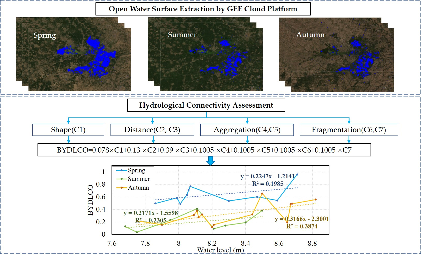
2.1. Study Area and Data
2.2. Methodology
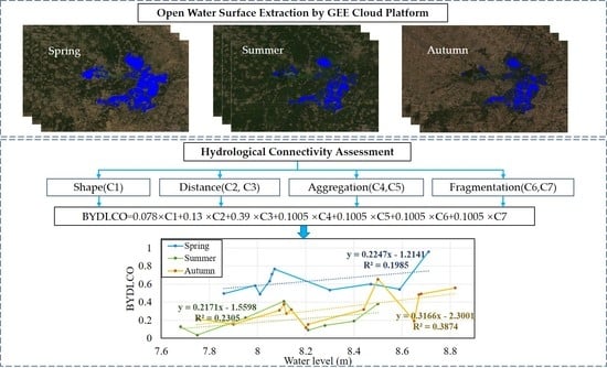
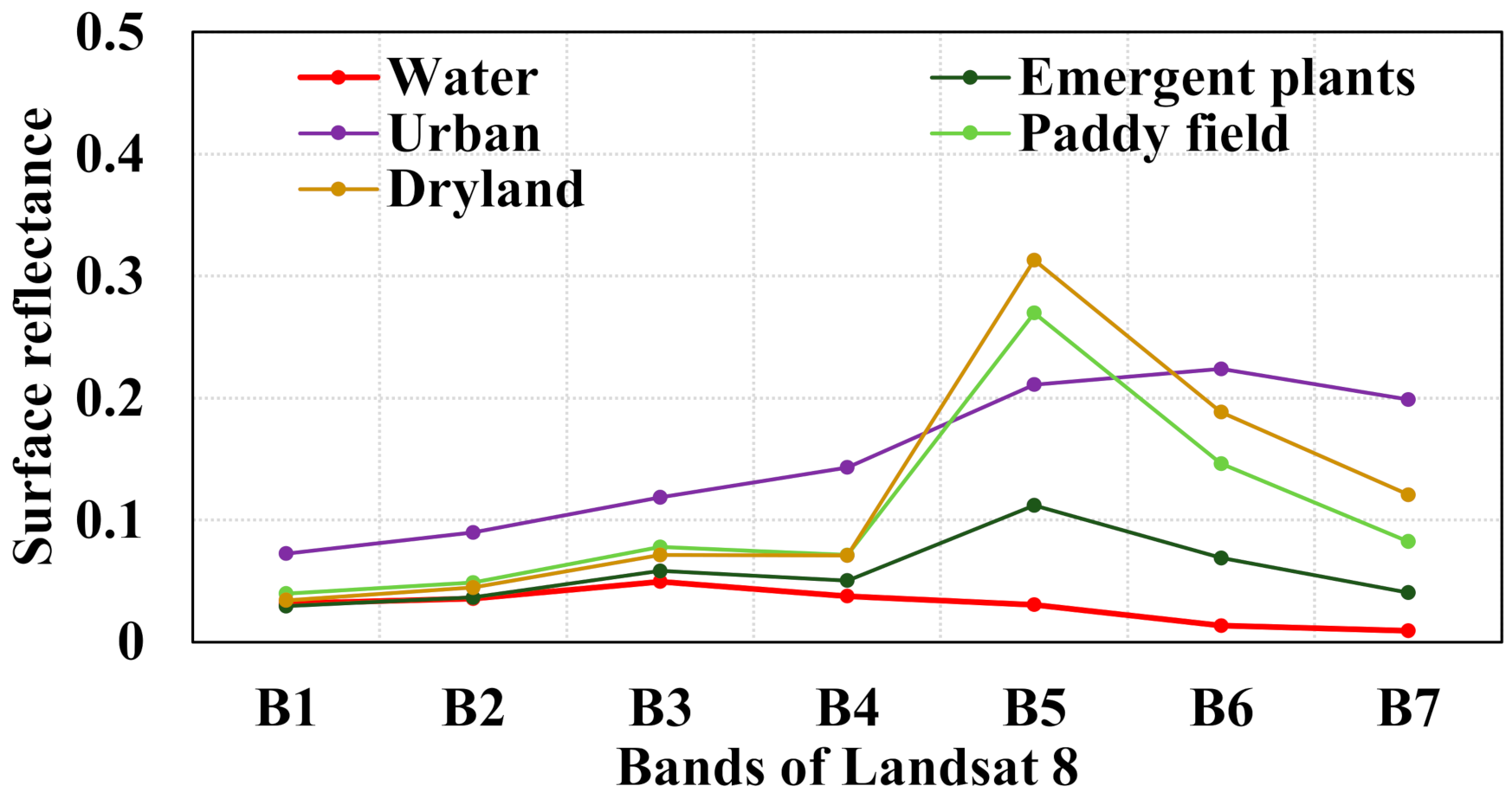
2.2.1. Surface Open Water Mapping
2.2.2. Assessment of Hydrological Connectivity in BYDL
3. Results
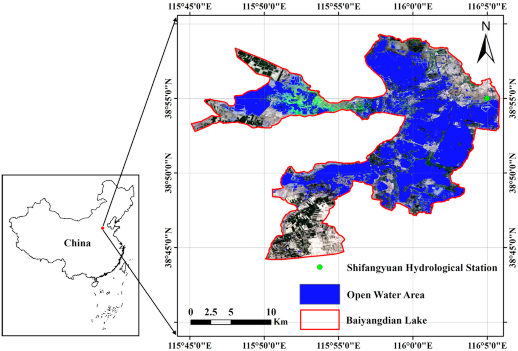
3.1. Comparison of Open Water Surface Extraction Methods
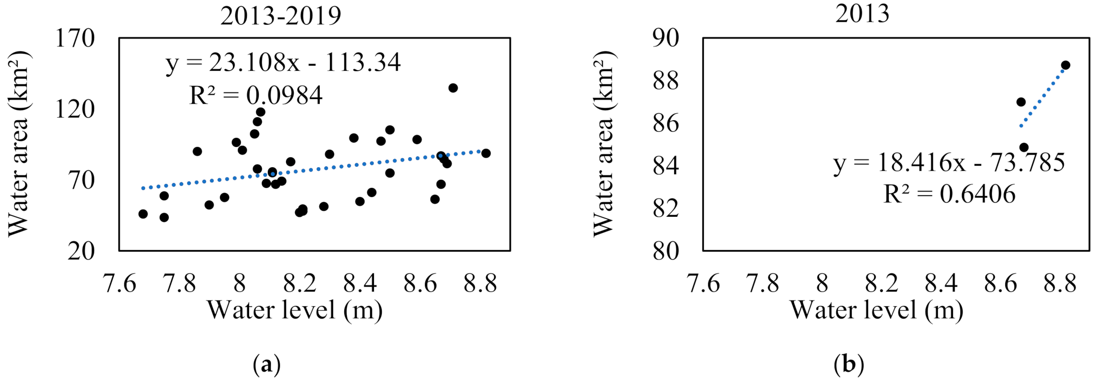
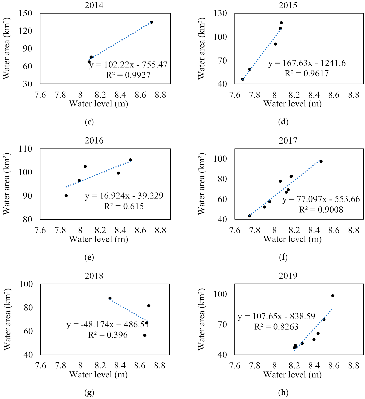
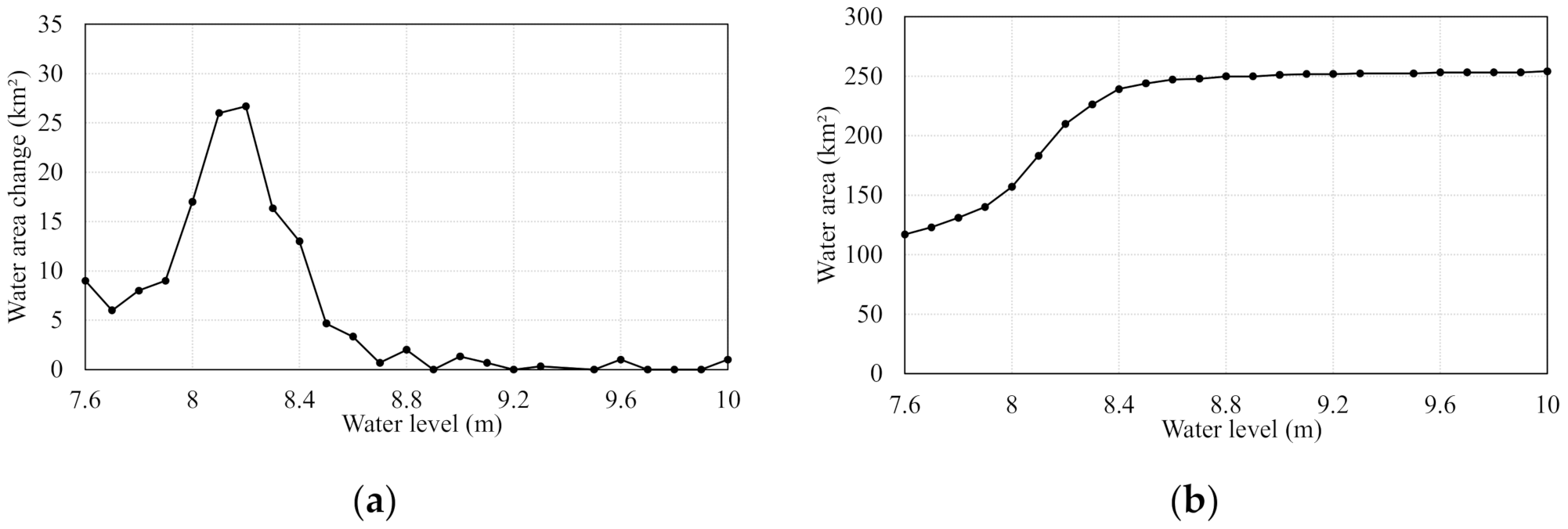
3.2. Variations in Open Water Surface with Water Level and Season
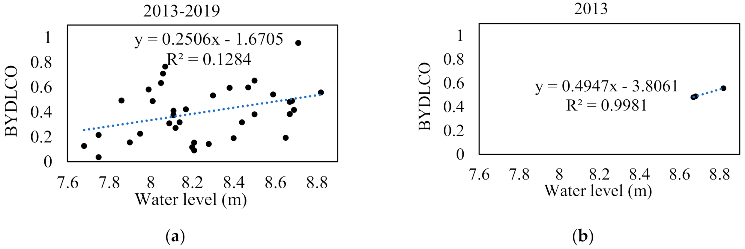
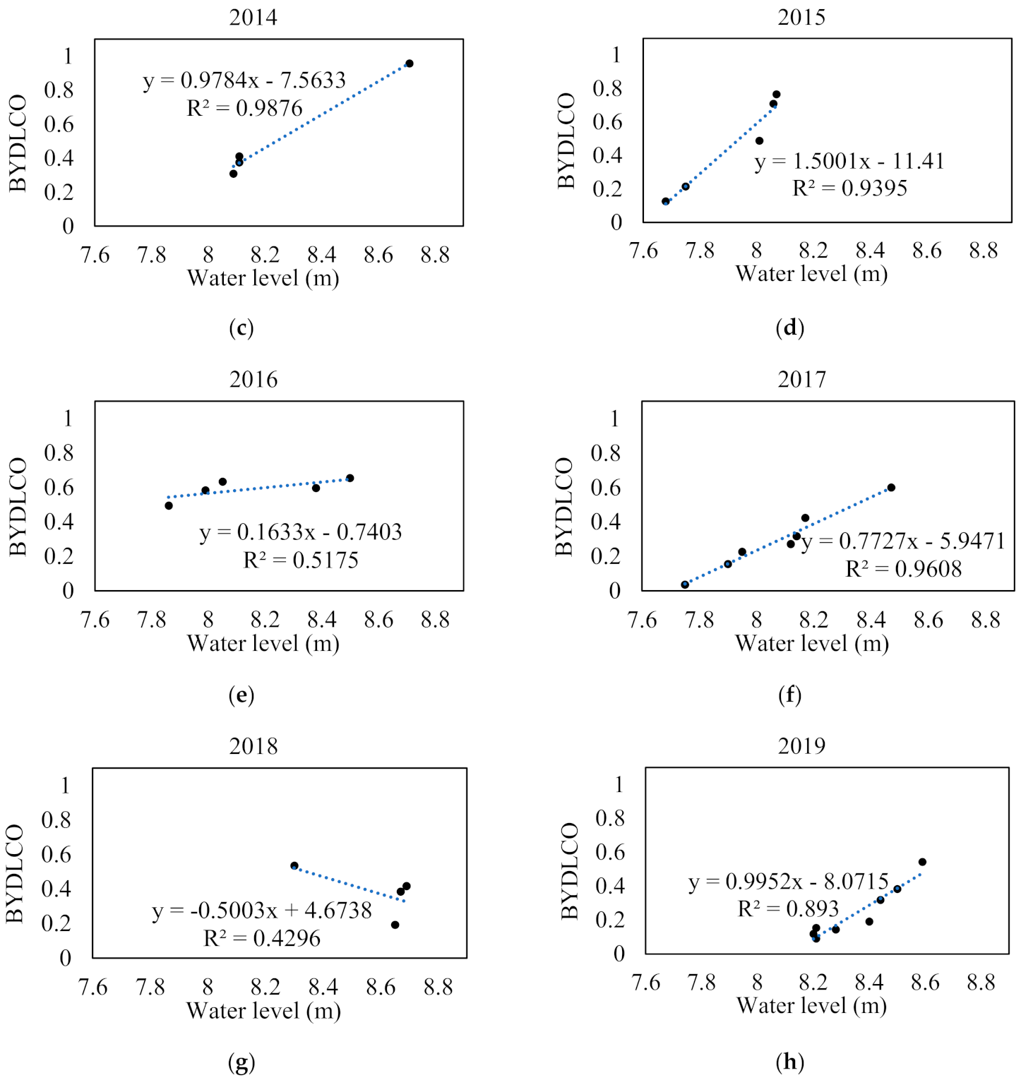
3.3. Temporal Variation in BYDL Hydrological Connectivity
4. Discussion
4.1. Accuracy of Extracting Open Water Area in BYDL from Landsat 8 Images
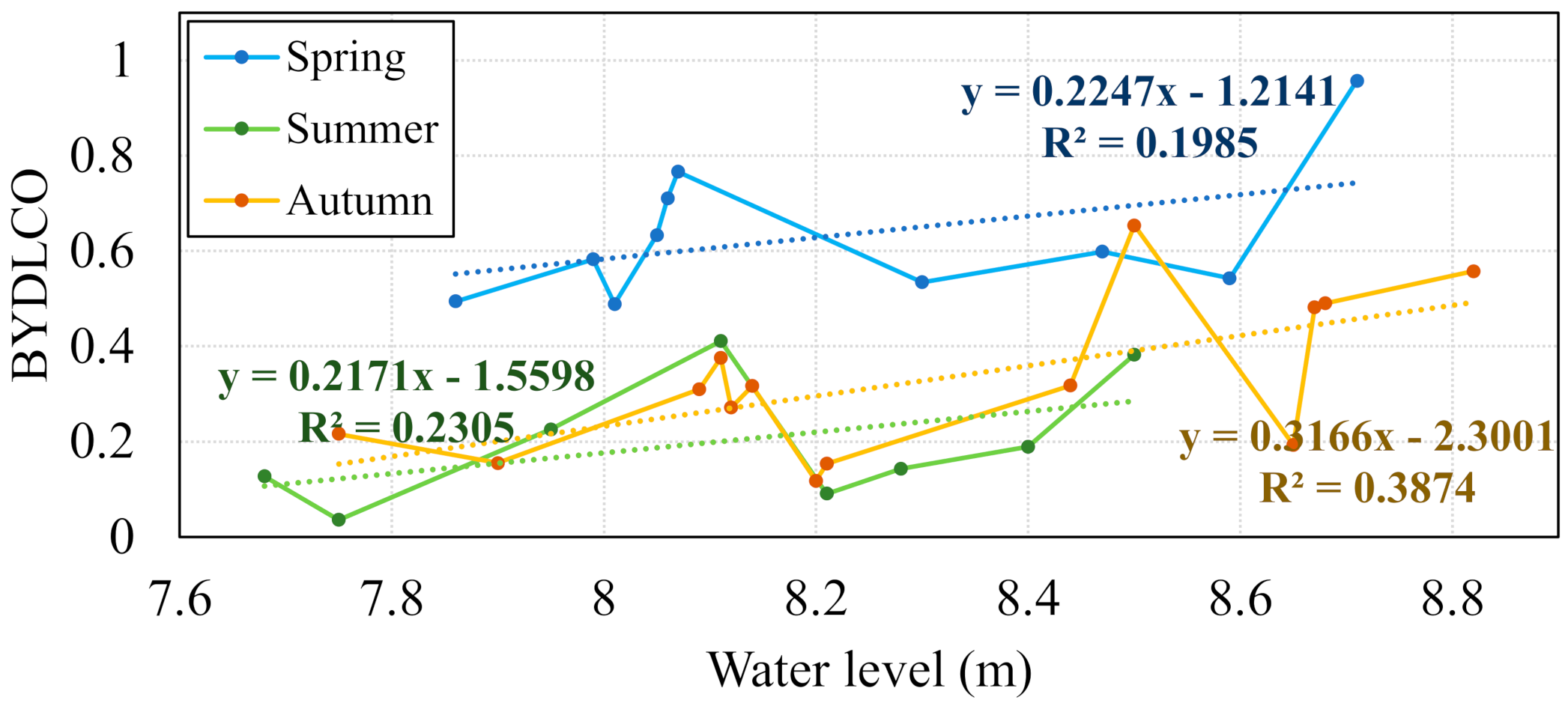
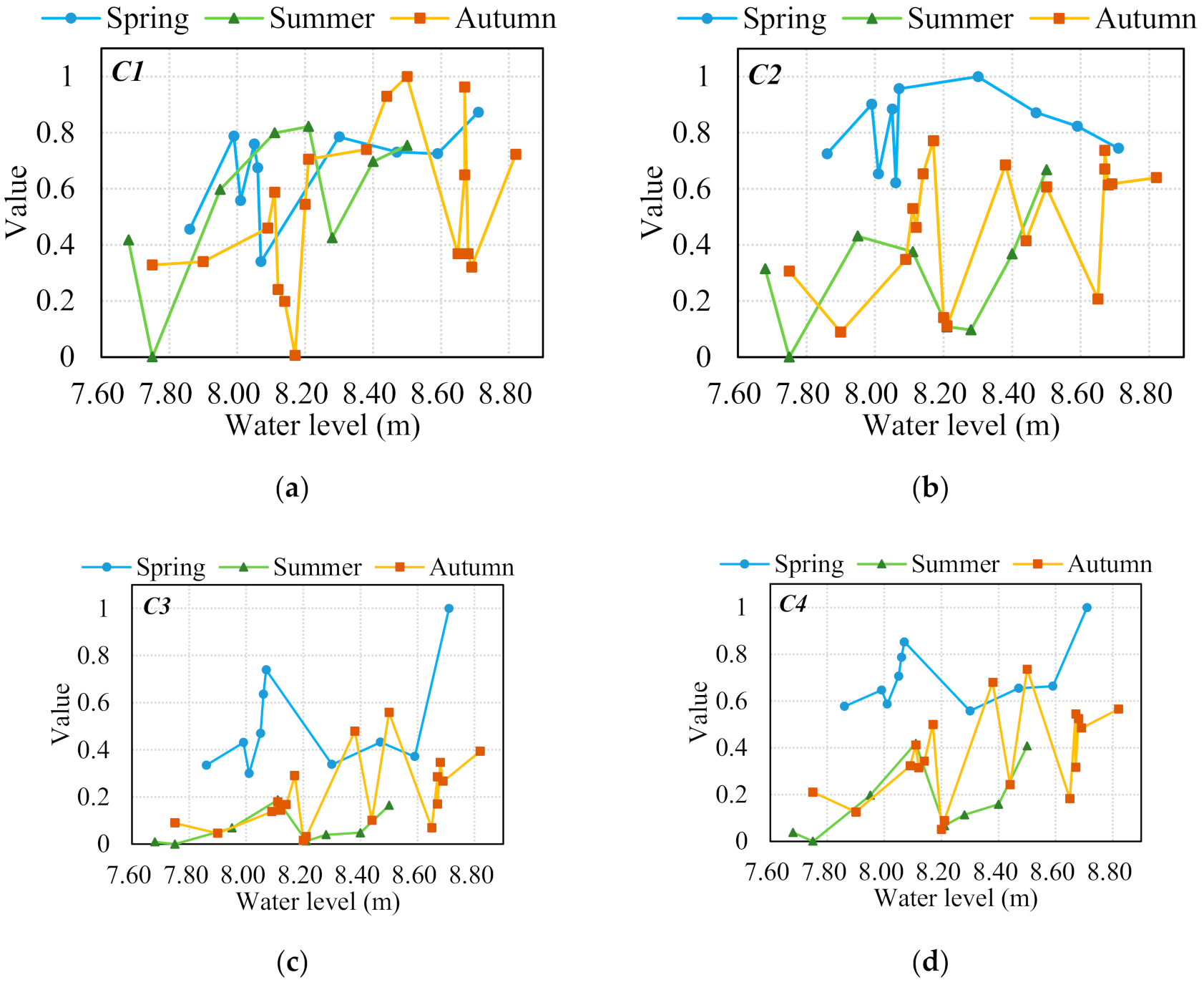
4.2. Interannual and Seasonal Variations in Hydrological Connectivity of BYDL
5. Conclusions
Author Contributions
Funding
Institutional Review Board Statement
Informed Consent Statement
Data Availability Statement
Conflicts of Interest
References
- Wang, X.; Shang, S.; Qu, Z.; Liu, T.; Melesse, A.M.; Yang, W. Simulated wetland conservation-restoration effects on water quantity and quality at watershed scale. J. Environ. Manag. 2010, 91, 1511–1525. [Google Scholar] [CrossRef]
- Vanderhoof, M.K.; Lane, C.R.; McManus, M.G.; Alexander, L.C.; Christensen, J.R. Wetlands inform how climate extremes influence surface water expansion and contraction. Hydrol. Earth Syst. Sci. 2018, 22, 1851–1873. [Google Scholar] [CrossRef]
- Junk, W.; Wantzen, K. The flood pulse concept: New aspects, approaches and applications—An update. Available online: https://www.researchgate.net/publication/274511459_The_Flood_Pulse_Concept_New_Aspects_Approaches_and_Applications-An_Update (accessed on 21 January 2021).
- Lane, C.R.; Leibowitz, S.G.; Autrey, B.C.; LeDuc, S.D.; Alexander, L.C. Hydrological, Physical, and Chemical Functions and Connectivity of Non-Floodplain Wetlands to Downstream Waters: A Review. JAWRA J. Am. Water Resour. Assoc. 2018, 54, 346–371. [Google Scholar] [CrossRef]
- Pringle, C.M. Hydrologic connectivity and the management of biological reserves: A global perspective. Ecol. Appl. 2001, 11, 981–998. [Google Scholar] [CrossRef]
- Bracken, L.J.; Croke, J. The concept of hydrological connectivity and its contribution to understanding runoff-dominated geomorphic systems. Hydrol. Process. Int. J. 2007, 21, 1749–1763. [Google Scholar] [CrossRef]
- Obolewski, K. Macrozoobenthos patterns along environmental gradients and hydrological connectivity of oxbow lakes. Ecol. Eng. 2011, 37, 796–805. [Google Scholar] [CrossRef]
- Dierauer, J.; Pinter, N.; Remo, J.W.F. Evaluation of levee setbacks for flood-loss reduction, Middle Mississippi River, USA. J. Hydrol. 2012, 450, 1–8. [Google Scholar] [CrossRef]
- Li, Y.; Zhang, Q.; Cai, Y.; Tan, Z.; Wu, H.; Liu, X.; Yao, J. Hydrodynamic investigation of surface hydrological connectivity and its effects on the water quality of seasonal lakes: Insights from a complex floodplain setting (Poyang Lake, China). Sci. Total Environ. 2019, 660, 245–259. [Google Scholar] [CrossRef]
- Xie, C.; Cui, B.; Xie, T.; Yu, S.; Liu, Z.; Chen, C.; Ning, Z.; Wang, Q.; Zou, Y.; Shao, X. Hydrological connectivity dynamics of tidal flat systems impacted by severe reclamation in the Yellow River Delta. Sci. Total Environ. 2020, 739, 139860. [Google Scholar] [CrossRef]
- Meng, B.; Liu, J.; Bao, K.; Sun, B. Methodologies and Management Framework for Restoration of Wetland Hydrologic Connectivity: A Synthesis. Integr. Environ. Assess. Manag. 2020, 16, 438–451. [Google Scholar] [CrossRef] [PubMed]
- Bracken, L.J.; Wainwright, J.; Ali, G.A.; Tetzlaff, D.; Smith, M.W.; Reaney, S.M.; Roy, A.G. Concepts of hydrological connectivity: Research approaches, pathways and future agendas. Earth Sci. Rev. 2013, 119, 17–34. [Google Scholar] [CrossRef]
- Rokni, K.; Ahmad, A.; Selamat, A.; Hazini, S. Water Feature Extraction and Change Detection Using Multitemporal Landsat Imagery. Remote Sens. 2014, 6, 4173–4189. [Google Scholar] [CrossRef]
- Pekel, J.F.; Cottam, A.; Gorelick, N.; Belward, A.S. High-resolution mapping of global surface water and its long-term changes. Nature 2016, 540, 418–422. [Google Scholar] [CrossRef]
- Bijeesh, T.V.; Narasimhamurthy, K.N. Surface water detection and delineation using remote sensing images: A review of methods and algorithms. Sustain. Water Resour. Manag. 2020, 6, 1–23. [Google Scholar] [CrossRef]
- Huang, C.; Chen, Y.; Zhang, S.; Wu, J. Detecting, Extracting, and Monitoring Surface Water From Space Using Optical Sensors: A Review. Rev. Geophys. 2018, 56, 333–360. [Google Scholar] [CrossRef]
- Ullah, M.; Li, J.; Wadood, B. Analysis of Urban Expansion and its Impacts on Land Surface Temperature and Vegetation Using RS and GIS, A Case Study in Xi’an City, China. Earth Syst. Environ. 2020, 4, 583–597. [Google Scholar] [CrossRef]
- Pathak, C.; Chandra, S.; Maurya, G.; Rathore, A.; Sarif, M.O.; Gupta, R.D. The Effects of Land Indices on Thermal State in Surface Urban Heat Island Formation: A Case Study on Agra City in India Using Remote Sensing Data (1992–2019). Earth Syst. Environ. 2020, 5, 135–154. [Google Scholar] [CrossRef]
- Most, M.V.D.; Hudson, P.F. The influence of floodplain geomorphology and hydrologic connectivity on alligator gar (Atractosteus spatula) habitat along the embanked floodplain of the Lower Mississippi River. Geomorphology 2018, 302, 62–75. [Google Scholar] [CrossRef]
- Long, C.M.; Pavelsky, T.M. Remote sensing of suspended sediment concentration and hydrologic connectivity in a complex wetland environment. Remote Sens. Environ. 2013, 129, 197–209. [Google Scholar] [CrossRef]
- Hudson, P.F.; Heitmuller, F.T.; Leitch, M.B. Hydrologic connectivity of oxbow lakes along the lower Guadalupe River, Texas: The influence of geomorphic and climatic controls on the “flood pulse concept”. J. Hydrol. 2012, 414, 174–183. [Google Scholar] [CrossRef]
- McFeeters, S.K. The use of the normalized difference water index (NDWI) in the delineation of open water features. Int. J. Remote Sens. 1996, 17, 1425–1432. [Google Scholar] [CrossRef]
- Jiang, H.; Feng, M.; Zhu, Y.; Lu, N.; Huang, J.; Xiao, T. An Automated Method for Extracting Rivers and Lakes from Landsat Imagery. Remote Sens. 2014, 6, 5067–5089. [Google Scholar] [CrossRef]
- Jia, K.; Jiang, W.; Li, J.; Tang, Z. Spectral matching based on discrete particle swarm optimization: A new method for terrestrial water body extraction using multi-temporal Landsat 8 images. Remote Sens. Environ. 2018, 209, 1–18. [Google Scholar] [CrossRef]
- Melack, J.M.; Hess, L.L. Remote Sensing of the Distribution and Extent of Wetlands in the Amazon Basin. In Amazonian Floodplain Forests; Springer: Berlin/Heidelberg, Germany, 2010; pp. 43–59. [Google Scholar]
- Schumann, G.J.P.; Moller, D.K. Microwave remote sensing of flood inundation. Phys. Chem. EarthParts A/B/C 2015, 83–84, 84–95. [Google Scholar] [CrossRef]
- Lang, M.W.; McCarty, G.W. Lidar Intensity for Improved Detection Of Inundation Below The Forest Canopy. Wetlands 2009, 29, 1166–1178. [Google Scholar] [CrossRef]
- Gala, T.S.; Melesse, A.M. Monitoring prairie wet area with an integrated LANDSAT ETM plus, RADARSAT-1 SAR and ancillary data from LIDAR. Catena 2012, 95, 12–23. [Google Scholar] [CrossRef]
- Lang, M.W.; Kim, V.; McCarty, G.W.; Li, X.; Yeo, I.; Huang, C.; Du, L. Improved Detection of Inundation below the Forest Canopy using Normalized LiDAR Intensity Data. Remote Sens. 2020, 12, 707. [Google Scholar] [CrossRef]
- Huang, C.; Peng, Y.; Lang, M.; Yeo, I.; McCarty, G. Wetland inundation mapping and change monitoring using Landsat and airborne LiDAR data. Remote Sens. Environ. 2014, 141, 231–242. [Google Scholar] [CrossRef]
- Jin, H.; Huang, C.; Lang, M.W.; Yeo, I.; Stehman, S.V. Monitoring of wetland inundation dynamics in the Delmarva Peninsula using Landsat time-series imagery from 1985 to 2011. Remote Sens. Environ. 2017, 190, 26–41. [Google Scholar] [CrossRef]
- Ordoyne, C.; Friedl, M.A. Using MODIS data to characterize seasonal inundation patterns in the Florida Everglades. Remote Sens. Environ. 2008, 112, 4107–4119. [Google Scholar] [CrossRef]
- Malinowski, R.; Groom, G.; Schwanghart, W.; Heckrath, G. Detection and Delineation of Localized Flooding from World View-2 Multispectral Data. Remote Sens. 2015, 7, 14853–14875. [Google Scholar] [CrossRef]
- Tockner, K.; Pennetzdorfer, D.; Reiner, N.; Schiemer, F.; Ward, J. Hydrological connectivity, and the exchange of organic matter and nutrients in a dynamic river–floodplain system (Danube, Austria). Freshw. Biol. 1999, 41, 521–535. [Google Scholar] [CrossRef]
- Park, E. Characterizing channel-floodplain connectivity using satellite altimetry: Mechanism, hydrogeomorphic control, and sediment budget. Remote Sens. Environ. 2020, 243, 111783. [Google Scholar] [CrossRef]
- Zhuang, C.; Ouyang, Z.; Xu, W.; Bai, Y.; Zhou, W.; Zheng, H.; Wang, X. Impacts of human activities on the hydrology of Baiyangdian Lake, China. Environ. Earth Sci. 2011, 62, 1343–1350. [Google Scholar] [CrossRef]
- Li, Y.; Wang, L.; Zheng, H.; Jin, H.; Xu, T.; Yang, P.; Tijiang, X.; Yan, Z.; Ji, Z.; Lu, J.; et al. Evolution Characteristics for Water Eco-Environment of Baiyangdian Lake with 3S Technologies in the Past 60 Years. In Proceedings of the International Conference on Computer and Computing Technologies in Agriculture; Springer: Berlin/Heidelberg, Germany, 2011; pp. 434–460. Available online: https://hal.inria.fr/hal-01361013/document (accessed on 20 March 2021).
- Park, E.; Latrubesse, E.M. The hydro-geomorphologic complexity of the lower Amazon River floodplain and hydrological connectivity assessed by remote sensing and field control. Remote Sens. Environ. 2017, 198, 321–332. [Google Scholar] [CrossRef]
- Liu, D.; Wang, X.; Zhang, Y.; Yan, S.; Cui, B.; Yang, Z. A Landscape Connectivity Approach for Determining Minimum Ecological Lake Level: Implications for Lake Restoration. Water 2019, 11, 2237. [Google Scholar] [CrossRef]
- Wang, X.; Wang, W.; Jiang, W.; Jia, K.; Rao, P.; Lv, J. Analysis of the Dynamic Changes of the Baiyangdian Lake Surface Based on a Complex Water Extraction Method. Water 2018, 10, 1616. [Google Scholar] [CrossRef]
- Stevaux, J.C.; Corradini, F.A.; Aquino, S. Connectivity processes and riparian vegetation of the upper Paraná River, Brazil. J. South. Am. Earth Sci. 2013, 46, 113–121. [Google Scholar] [CrossRef]
- You, X.; Liu, J.; Zhang, L. Ecological modeling of riparian vegetation under disturbances: A review. Ecol. Model. 2015, 318, 293–300. [Google Scholar] [CrossRef]
- Liu, X.; Zhang, Q.; Li, Y.; Tan, Z.; Werner, A.D. Satellite image-based investigation of the seasonal variations in the hydrological connectivity of a large floodplain (Poyang Lake, China). J. Hydrol. 2020, 585, 124810. [Google Scholar] [CrossRef]
- Cabezas, A.; Gonzalez-Sanchis, M.; Gallardo, B.; Comin, F.A. Using continuous surface water level and temperature data to characterize hydrological connectivity in riparian wetlands. Environ. Monit. Assess. 2011, 183, 485–500. [Google Scholar] [CrossRef] [PubMed]
- Wright, K.; Hiatt, M.; Passalacqua, P. Hydrological Connectivity in Vegetated River Deltas: The Importance of Patchiness Below a Threshold. Geophys. Res. Lett. 2018, 45, 10416–10427. [Google Scholar] [CrossRef]
- Zhu, M.; Wang, S.; Kong, X.; Zheng, W.; Feng, W.; Zhang, X.; Yuan, R.; Song, X.; Sprenger, M. Interaction of Surface Water and Groundwater Influenced by Groundwater Over-Extraction, Waste Water Discharge and Water Transfer in Xiong’an New Area, China. Water 2019, 11, 539. [Google Scholar] [CrossRef]
- Bai, J.; Guan, Y.; Liu, P.; Zhang, L.; Cui, B.; Li, X.; Liu, X. Assessing the safe operating space of aquatic macrophyte biomass to control the terrestrialization of a grass-type shallow lake in China. J. Environ. Manag. 2020, 266, 110479. [Google Scholar] [CrossRef]
- Cui, G.; Liu, Y.; Tong, S. Analysis of the causes of wetland landscape patterns and hydrological connectivity changes in Momoge National Nature Reserve based on the Google Earth Engine Platform. Arab. J. Geosci. 2021, 14, 1–16. [Google Scholar] [CrossRef]
- Busker, T.; Roo, A.; Gelati, E.; Schwatke, C.; Adamovic, M.; Bisselink, B.; Pekel, J.F.; Cottam, A. A global lake and reservoir volume analysis using a surface water dataset and satellite altimetry. Hydrol. Earth Syst. Sci. 2019, 23, 669–690. [Google Scholar] [CrossRef]
- Schultz, G.A.; Engman, E.T. Remote Sensing in Hydrology and Water Management; Springer: Berlin Heidelberg, Germany, 2000. [Google Scholar]
- Xu, H. A Study on Information Extraction of Water Body with the Modified Normalized Difference Water Index (MNDWI). J. Remote Sens. 2005, 9, 589–595. [Google Scholar]
- Feyisa, G.L.; Meilby, H.; Fensholt, R.; Proud, S.R. Automated Water Extraction Index: A new technique for surface water mapping using Landsat imagery. Remote Sens. Environ. 2014, 140, 23–35. [Google Scholar] [CrossRef]
- Fisher, A.; Flood, N.; Danaher, T. Comparing Landsat water index methods for automated water classification in eastern Australia. Remote Sens. Environ. 2016, 175, 167–182. [Google Scholar] [CrossRef]
- Prewitt, J.M.; Mendelsohn, M.L. The analysis of cell images. Ann. New York Acad. Sci. 1966, 128, 1035–1053. [Google Scholar] [CrossRef]
- Otsu, N. A Threshold Selection Method from Gray-Level Histograms. IEEE Trans. Syst. Man. Cybern. 2007, 9, 62–66. [Google Scholar] [CrossRef]
- Congalton, R.G. A review of assessing the accuracy of classifications of remotely sensed data. Remote Sens. Environ. 1991, 37, 270–279. [Google Scholar] [CrossRef]
- Baker, W.L.; Cai, Y. The r. le programs for multiscale analysis of landscape structure using the GRASS geographical information system. Landsc. Ecol. 1992, 7, 291–302. [Google Scholar] [CrossRef]
- Weldon, A.J.; Haddad, N.M. The effects of patch shape on Indigo Buntings: Evidence for an ecological trap. Ecology 2005, 86, 1422–1431. [Google Scholar] [CrossRef]
- Yue, T.; Xu, B.; Liu, J. A patch connectivity index and its change in relation to new wetland at the Yellow River Delta. Int. J. Remote Sens. 2004, 25, 4617–4628. [Google Scholar] [CrossRef]
- McGarigal, K.M. FRAGSTATS: Spatial Pattern Analysis Program for Quantifying Landscape Structure; US Department of Agriculture, Forest Service, Pacific Northwest Research Station: Portland, OR, USA, 1995; Volume 351.
- Saura, S.; Pascual-Hortal, L. A new habitat availability index to integrate connectivity in landscape conservation planning: Comparison with existing indices and application to a case study. Landsc. Urban Plan. 2007, 83, 91–103. [Google Scholar] [CrossRef]
- Smith, B.; Wilson, J.B. A consumer’s guide to evenness indices. Oikos 1996, 76, 70–82. [Google Scholar] [CrossRef]
- De Macedo-Soares, P.; Petry, A.; Farjalla, V.; Caramaschi, E. Hydrological connectivity in coastal inland systems: Lessons from a Neotropical fish metacommunity. Ecol. Freshw. Fish. 2010, 19, 7–18. [Google Scholar] [CrossRef]
- He, H.S.; DeZonia, B.E.; Mladenoff, D.J. An aggregation index (AI) to quantify spatial patterns of landscapes. Landsc. Ecol. 2000, 15, 591–601. [Google Scholar] [CrossRef]
- Nafi’Shehab, Z.; Jamil, N.R.; Aris, A.Z.; Shafie, N.S. Spatial variation impact of landscape patterns and land use on water quality across an urbanized watershed in Bentong, Malaysia. Ecol. Indic. 2021, 122, 107254. [Google Scholar]
- Jaeger, J.A. Landscape division, splitting index, and effective mesh size: New measures of landscape fragmentation. Landsc. Ecol. 2000, 15, 115–130. [Google Scholar] [CrossRef]
- Saura, S.; Torné, J. Conefor Sensinode 2.2: A software package for quantifying the importance of habitat patches for landscape connectivity. Environ. Model. Softw. 2008, 24, 135–139. [Google Scholar] [CrossRef]
- Zhang, T.; Ren, H.; Qin, Q.; Zhang, C.; Sun, Y. Surface water extraction from Landsat 8 OLI imagery using the LBV transformation. IEEE J. Sel. Top. Appl. Earth Obs. Remote Sens. 2017, 10, 4417–4429. [Google Scholar] [CrossRef]
- Tang, C.; Yi, Y.; Yang, Z.; Zhou, Y.; Zerizghi, T.; Wang, X.; Cui, X.; Duan, P. Planktonic indicators of trophic states for a shallow lake (Baiyangdian Lake, China). Limnologica 2019, 78, 125712. [Google Scholar] [CrossRef]
- Yang, L.; Chen, S.; Lu, Y.; Yao, M. The Assessment of Hydrochemistry Characteristics and Eutrophication Level of Lake Baiyangdian, North of China. Available online: https://www.scientific.net/AMR.864-867.2357 (accessed on 21 January 2021).
- Han, Z.; Cui, B. Performance of macrophyte indicators to eutrophication pressure in ponds. Ecol. Eng. 2016, 96, 8–19. [Google Scholar] [CrossRef]
- Yin, J.; Cheng, W.; Yan, L.; Chen, X. Change of water resources in the Baiyangdian Wetland. Water Resour. Prot. 2009, 25, 52–58. [Google Scholar]
- Liu, D.; Wang, X.; Aminjafari, S.; Yang, W.; Cui, B.; Yan, S.; Zhang, Y.; Zhu, J.; Jaramillo, F. Using InSAR to identify hydrological connectivity and barriers in a highly fragmented wetland. Hydrol. Process. 2020, 34, 4417–4430. [Google Scholar] [CrossRef]
- Sun, W.; Ishidaira, H. Prospects for Extracting River Cross-sectional Information From High Resolution DSM Generated from ALOS PRISM Data. Available online: https://www.jstage.jst.go.jp/article/jshwr/22/0/22_0_88/_pdf (accessed on 21 January 2021).
- Huang, C.; Chen, Y.; Zhang, S.; Li, L.; Shi, K.; Liu, R. Spatial Downscaling of Suomi NPP–VIIRS Image for Lake Mapping. Water 2017, 9, 834. [Google Scholar] [CrossRef]
- Shah, C.A. Automated Lake Shoreline Mapping at Subpixel Accuracy. IEEE Geosci. Remote Sens. Lett. 2011, 8, 1125–1129. [Google Scholar] [CrossRef]
- Hudson, P.; Sounny-Slitine, M.; LaFevor, M. A new longitudinal approach to assess hydrologic connectivity: Embanked floodplain inundation along the lower Mississippi River. Hydrol. Process. 2013, 27, 2187–2196. [Google Scholar] [CrossRef]
- Bertoldi, W.; Drake, N.A.; Gurnell, A.M. Interactions between river flows and colonizing vegetation on a braided river: Exploring spatial and temporal dynamics in riparian vegetation cover using satellite data. Earth Surf. Process. Landf. 2011, 36, 1474–1486. [Google Scholar] [CrossRef]
- Zhang, Y.; Wang, X.; Li, C.; Cai, Y.; Yang, Z.; Yi, Y. NDVI dynamics under changing meteorological factors in a shallow lake in future metropolitan, semiarid area in North China. Sci. Rep. 2018, 8, 1–13. [Google Scholar] [CrossRef] [PubMed]
- Wang, C.; Zhu, P.; Wang, P.-f.; Zhang, W.-m. Effects of aquatic vegetation on flow in the Nansi Lake and its flow velocity modeling. J. Hydrodyn. 2006, 18, 640–648. [Google Scholar] [CrossRef]
- Kothyari, U.C.; Hayashi, K.; Hashimoto, H. Drag coefficient of unsubmerged rigid vegetation stems in open channel flows. J. Hydraul. Res. 2009, 47, 691–699. [Google Scholar] [CrossRef]
- Yi, Y.; Xie, H.; Yang, Y.; Zhou, Y.; Yang, Z. Suitable habitat mathematical model of common reed (Phragmites australis) in shallow lakes with coupling cellular automaton and modified logistic function. Ecol. Model. 2020, 419, 108938. [Google Scholar] [CrossRef]


| Band | Description | Wavelength (μm) |
|---|---|---|
| Blue Band | 0.45–0.51 | |
| Green Band | 0.53–0.59 | |
| Red Band | 0.64–0.67 | |
| Near-infrared Band | 0.85–0.88 | |
| Shortwave infrared Band 1 | 1.57–1.65 | |
| Shortwave infrared Band 2 | 2.11–2.29 |
| Aspect | Index | Interpretations |
|---|---|---|
| Shape | Related circumscribing circle (C1) | Movement efficiency within a water patch. |
| Distance | Euclidean nearest neighbor distance (C2) | Mean distance between water patches. |
| Probability of connectivity (C3) | Possibility of connection between patches. | |
| Aggregation | Shannon’s evenness index (C4) | Evenness of water patch distribution in the landscape. |
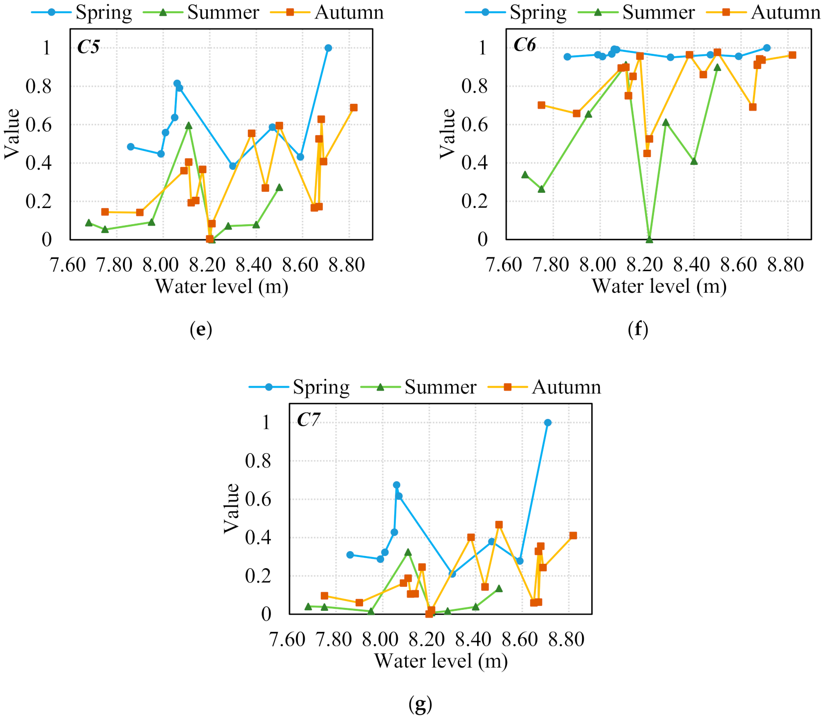
| Aggregation index (C5) | Like adjacency among water patches | |
| Fragmentation | Splitting index (C6) | Fragmentation degree of water patches |
| Average area (C7) | Average water patch area. |
| Date | Water Level (m) | Water Indexes | |||||||
|---|---|---|---|---|---|---|---|---|---|
| NDWI | MNDWI | AWEIsh | AWEInsh | WI2015 | NIR | NIR | NIR | ||
| Threshold for Open Water Surface | |||||||||
| >−0.049 | >0.251 | >0.005 | >0.024 | >3.219 | <0.007 | Based on Otsu Method | Based on 2-Mode Method | ||
| 22 August 2015 | 7.68 | 0.9650 | 0.9775 | 0.9475 | 0.9775 | 0.9475 | 0.9925 | 0.9950 | 0.9875 |
| 28 September 2017 | 7.90 | 0.9775 | 0.9825 | 0.9650 | 0.9825 | 0.9600 | 0.9875 | 0.9900 | 0.9900 |
| 30 June 2019 | 8.21 | 0.9750 | 0.9700 | 0.9650 | 0.9700 | 0.9625 | 0.9925 | 0.9875 | 0.9925 |
| 4 March 2017 | 8.47 | 0.9725 | 0.9675 | 0.9700 | 0.9675 | 0.9700 | 0.9750 | 0.9750 | 0.9750 |
| 28 November 2016 | 8.50 | 0.9850 | 0.9725 | 0.9825 | 0.9775 | 0.9850 | 0.9825 | 0.9800 | 0.9900 |
| 3 October 2013 | 8.82 | 0.9825 | 0.9825 | 0.9850 | 0.9850 | 0.9850 | 0.9350 | 0.9775 | 0.9850 |
| 3 December 2018 | 8.69 | 0.9875 | 0.6000 | 0.8775 | 0.6075 | 0.8325 | 0.9950 | 0.9925 | 0.9925 |
| Average | 0.9779 | 0.9218 | 0.9561 | 0.9239 | 0.9489 | 0.9800 | 0.9854 | 0.9875 | |
| Standard deviation | 0.0078 | 0.1420 | 0.0368 | 0.1397 | 0.0531 | 0.0210 | 0.0078 | 0.0061 | |
Publisher’s Note: MDPI stays neutral with regard to jurisdictional claims in published maps and institutional affiliations. |
© 2021 by the authors. Licensee MDPI, Basel, Switzerland. This article is an open access article distributed under the terms and conditions of the Creative Commons Attribution (CC BY) license (http://creativecommons.org/licenses/by/4.0/).
Share and Cite
Li, Z.; Sun, W.; Chen, H.; Xue, B.; Yu, J.; Tian, Z. Interannual and Seasonal Variations of Hydrological Connectivity in a Large Shallow Wetland of North China Estimated from Landsat 8 Images. Remote Sens. 2021, 13, 1214. https://doi.org/10.3390/rs13061214
Li Z, Sun W, Chen H, Xue B, Yu J, Tian Z. Interannual and Seasonal Variations of Hydrological Connectivity in a Large Shallow Wetland of North China Estimated from Landsat 8 Images. Remote Sensing. 2021; 13(6):1214. https://doi.org/10.3390/rs13061214
Chicago/Turabian StyleLi, Ziqi, Wenchao Sun, Haiyang Chen, Baolin Xue, Jingshan Yu, and Zaifeng Tian. 2021. "Interannual and Seasonal Variations of Hydrological Connectivity in a Large Shallow Wetland of North China Estimated from Landsat 8 Images" Remote Sensing 13, no. 6: 1214. https://doi.org/10.3390/rs13061214
APA StyleLi, Z., Sun, W., Chen, H., Xue, B., Yu, J., & Tian, Z. (2021). Interannual and Seasonal Variations of Hydrological Connectivity in a Large Shallow Wetland of North China Estimated from Landsat 8 Images. Remote Sensing, 13(6), 1214. https://doi.org/10.3390/rs13061214