Abstract
Synthetic aperture radar (SAR) is a significant application in maritime monitoring, which can provide SAR data throughout the day and in all weather conditions. With the development of artificial intelligence and big data technologies, the data-driven convolutional neural network (CNN) has become widely used in ship detection. However, the accuracy, feature visualization, and analysis of ship detection need to be improved further, when the CNN method is used. In this letter, we propose a two-stage ship detection for land-contained sea area without a traditional sea-land segmentation process. First, to decrease the possibly existing false alarms from the island, an island filter is used as the first step, and then threshold segmentation is used to quickly perform candidate detection. Second, a two-layer lightweight CNN model-based classifier is built to separate false alarms from the ship object. Finally, we discuss the CNN interpretation and visualize in detail when the ship is predicted in vertical–horizontal (VH) and vertical–vertical (VV) polarization. Experiments demonstrate that the proposed method can reach an accuracy of 99.4% and an F1 score of 0.99 based on the Sentinel-1 images for a ship with a size of less than 32 × 32.
1. Introduction
Ship detection plays a crucial role in maritime transportation, maritime surveillance applications in fishing, and maritime rights maintenance. Synthetic aperture radar (SAR), as active remote sensing, is most suitable for ship detection because it is sensitive to hard targets. Furthermore, SAR works throughout the day and in all weather conditions. In recent years, many SAR satellites, such as Radarsat1/2, TerraSAR-X, Sentinel-1, COSMO-SkyMed, and GF-3, have been providing a wide variety of SAR images with different resolutions, modes, and polarizations for maritime application, thereby enabling ship detection.
According to previous research, ship detection usually involves land-ocean segmentation, preprocessing, prescreening, and discrimination. Constant false alarm rate (CFAR) [1,2,3,4], as a traditional method, is typically used in ship detection. Furthermore, these methods are dependent on the statistical distribution of sea clutter, which is difficult to accurately estimate because of sea waves and ocean currents. Besides, the window size of protection and background influences the detection effectiveness. Land-ocean segmentation is also unavoidable, thereby causing poor robustness for SAR imagery in those methods. These traditional ship-detection methods require extensive calculations to address the parameters of statistical distribution, which is not sufficiently flexible and intelligent, and the detection speed does not meet actual needs.
At present, with the development of big data and deep learning technologies, convolutional neural networks (CNN) are widely used in mapping ice-wedge polygon (IWP) [5,6], identifying damaged buildings [7], classifying sea ice cover and land type [8,9,10], and so on. Those CNN models successfully developed an automatic extraction framework for high spatial resolution remote sensing applications in a large-scale application. However, those CNN models need the input data and ground truth annotation one-to-one correspondence. In some research fields, the ground truth data are not easy to obtain due to lack of expert knowledge and time consumption. Besides, a growing number of researchers are beginning to study object detection based on convolutional neural network (CNN) methods. Single-stage methods, such as a proposed region-based convolutional network (R-CNN) [11], Fast R-CNN [12], and Faster R-CNN [13], and two-stage methods such as SSD [14], YOLO V1/V2/V3/V4 [14,15,16,17,18], and RetinaNet [19], have exhibited impressive results on various object detection benchmarks based on PASCAL VOC [20] and MS COCO [21] datasets. However, the natural images differ from the SAR images, which are produced through a coherent imaging process that leads to foreshortening, layover, and shadowing. Apart from the image mechanisms, targets in SAR images vary, such as ghosts, islands, artificial objects, island, or a harbor that displays similar backscattering mechanisms to ships, which lead to a high rate of false alarms. Therefore, to apply the deep learning algorithm to the SAR data, researchers have constructed SAR Ship Detection Dataset [22], SAR-Ship-Dataset [23], OpenSAR [24], and high-resolution SAR image dataset [25] containing Sentinel-1, Radarsat-2, TerraSAR-X, COSMO-SkyMe, and GaoFen-3 images. These datasets vary in polarization (HH, HV, VH, and VV), resolution (0.5, 1, 3, 5, 8, and 10 m), incidence angle, imaging mode, and background.
Compared with the PASCAL and COCO datasets, the SAR datasets have a low volume. When training the object detectors for ship detection in SAR images, finetuning or transfer learning is widely used. These CNN methods have been used for target detection in SAR images, ship detection [26], and land target detection [27], and have performed better than the traditional methods.
The deficiency of the method is that average precision is low because the models fail to consider the SAR image mechanisms [22]. However, the pretraining time and detection speed of classical object detectors usually do not meet the requirements of real-time ship detection, maritime rescue, and emergency military decision-making. In recent years, many researchers have paid attention to ship detection using CNN objectors. A grid CNN was proposed and proved to improve the accuracy and speed of ship detection [28]. Receptive pyramid network extraction strategies and attention mechanism technology are proved to improve the accuracy of ship detection [29]. These methods have relatively deep convolutional layers, hundreds of millions of parameters, and involve a long training time. Besides, in the data-driven CNN model, it is not easy and time-consuming to obtain the true value of the target bounding box corresponding to the input image. Therefore, these methods do not meet the requirements of fast processing, real-time response, and large-scale detection.
To achieve low complexity and high reliability through a CNN, some researchers have begun to split the images into small patches in the pre-screening stage and then use a relatively lightweight CNN model to classify the patches. Thereafter, the classification results are mapped onto the original images. A two-stage framework involves pre-screening and a relatively simple CNN architecture have been proposed [30,31], but in the pre-screening stage where a simple constant false alarm rate detector is used. As mentioned, the CFAR detector falls into a large number of calculations to solve the parameters of the statistical distribution and ignores small targets. Six convolutional layers, three max-pooling layers, and two full-connection layers are proposed to ship classification based on GF3-SAR images [26]. In these methods, CFAR and Ostu are typically used to obtain candidate targets in the pre-screening stage, and then a simple CNN model is used to reduce false alarms and recognize the ship. Unfortunately, time consumption is increased when sea-land segmentation and CFAR detector are applied in the pre-screening stage. Although the Ostu improves the speed of the pre-screening stage, the threshold may not work effectively and may cause an excessive number of false alarms. After the SAR image preprocessing, the CNN model can perform ship detection from all patches, but the accuracy of ship detection needs to be improved for the small-level ship. Besides, scholars had analyzed and discussed the ship detection in the CNN method, but the feature visualization and analysis of ship detection in both VH and VV polarization were less discussed, which is important in understanding ship detection through the CNN method. Thus, in this letter, we are mainly concerned with ship detection accuracy and feature visualization and analysis by using the VH and VV polarization.
Considering these difficulties, we propose a two-stage ship-detection method. In the first stage, Lee and island filters are used to reduce the noise and false alarms. Then, an exponential inverse cumulative distribution function (EICDF) [32,33] is applied to quickly estimate the segmentation threshold and obtain candidate detection results with relatively few false alarms. Then, all candidates are put in a lightweight CNN to accurately recognize the ships. Finally, the feature visualization and analysis of ship detection are carried out by the Grad-class activation mapping (Grad-CAM). The main contributions of the work are as follows:
- The first ship detection method for SAR images is proposed. To quickly obtain candidate detection results, this study presents a fast threshold segmentation for candidate detection, which has been proved to reduce false alarms, obtain all candidate ships with different scales, and save time in the offshore area.
- Most detectors consist of deep architecture and millions of parameters, thereby resulting in complex extraction features and lengthy pretraining time. In this study, a simple lightweight CNN architecture, which is fast and effective, was proposed to detect the ship.
- The Grad-CAM was introduced to explain and visualize the CNN model, and then analyze the great attention pixel when the ship and false alarm were predicted.
The rest of this paper is organized as follows. In Section 2, we present the details of the dataset, data pre-processing, and the proposed method. Section 3 reports the experiment results. Section 4 and Section 5 present the discussion and conclusions, respectively. Finally, a summary of this paper is provided.
2. Dataset and Proposed Methodology
In this section, first, the Sentinel-1 SAR images are introduced in detail. Second, the data progress, candidate targets, and dataset conduction are described. Third, the lightweight CNN model is presented.
2.1. Dataset
In this section, three Sentinel-1 SAR images located in the East Sea of China and one Sentinel-1SAR image located in the Huanghai Sea were used in the experiment as shown in Figure 1. The SAR images contain VH and VV polarizations with a pixel resolution of 10 m × 10 m, and the real resolution is 22 m × 20 m in azimuth and range. The information of SAR images includes the acquisition time of the image, the swath width, and the image mode is presented in Table 1.
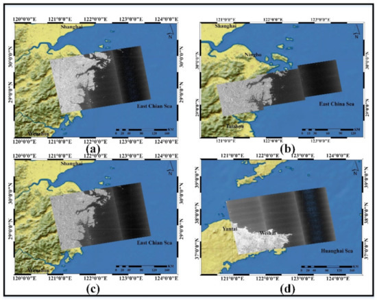
Figure 1.
Image coverage of three Sentinel-1 images: (a) 23 June 2020; (b) 11 July 2020; (c) 17 July 2020; (d) 13 February 2021.

Table 1.
Detailed information of Sentinel-1.
2.2. Data Pre-Processing
In the section, the process of Sentinel-1 SAR images is described in detail. Figure 2 shows the complete workflow of ship detection. The workflow consists of four steps: pre-processing, candidate target and dataset construction, CNN model building, and training and ship detection.
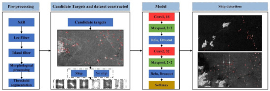
Figure 2.
Workflow of ship detection.
The presence of speckle noise in SAR images causes difficulty in interpretation, thereby degrading the image quality. Therefore, the refined Lee filter [34] was used to improve the quality of the image and eliminate the coherence noise before the SAR image input (Figure 3a). In previous research, land-ocean segmentation was unavoidable in the pre-process to reduce the false alarms from land, harbor, and island. In the SAR images, the false alarms are mainly from stones, rocks, artificial targets, and island can usually provide similar backscatter coefficients of ships. Therefore, the island filter is applied to reduce the false alarms from the island, which is proved effective [30,35], as shown in Figure 3b. The ship candidates on the dark sea surface are reserved, and similar changes are visible on the edge of the island and reef (see Figure 3c). In summary, the false alarm of the island and reef is reduced more than that of the ship, leading to an increase in the ship-island contrast. To achieve ship target enhancement, we applied the morphological process consisting of erosion and dilation to improve contrast (see Figure 3d). Generally, the ship for detection is assumed to fit a permanent distribution, and then the threshold is calculated through probability density function. Similar to the CFAR method, after the morphological process, the image is similar to exponent distribution, and then the threshold is estimated by EICDF method with the input image mean value and a priori value of 0.999. The segmentation result is shown in Figure 3e. Finally, eight-connected domain processing was applied in the segmentation, and the preliminary result is shown in Figure 3f. After eight-connected domain processing, we can get the minimum bounding rectangle of the candidate target. Then, we can obtain all candidate slices according to the minimum bounding rectangle. Noteworthy, taken the centroid of the target as the origin, the slices are extended to 32 × 32 for the minimum bounding rectangle less than 32 × 32 and the slices are resized 32 × 32 for the minimum bounding rectangle of more than 32 × 32.
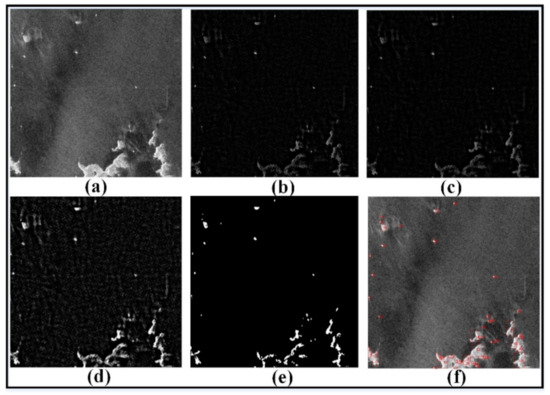
Figure 3.
Pre-processing of SAR image: (a) SAR image, (b) image of island filter, (c) image of Gaussian filter, (d) image of the morphological process, (e) binary image, and (f) candidate result.
2.3. Candidate Detection
In this section, the candidate detection is discussed in detail based on the threshold calculation. In the candidate detection stage, the SAR images acquired on 11 July 2020 (No.2) and 17 July 2020 (No.3) were used. The two SAR images were cropped into 1000 × 1000 sub-images, with 50% overlap, then all sub-images were preprocessed according to the data-process method described above. Figure 4a shows four SAR image background scenes with the size of 1000 × 1000 in the flow of candidate detection. Scene 1, screen 2, and screen 3 include different land and islands and different scale ships, and scene 4 includes ships in inhomogeneous conditions. The contrast between the candidate target and sea background of the SAR data is more obvious after data preprocessing. Thus, we had an opportunity to detect the targets using the traditional method. The CFAR was proved available when it was used to detect the candidates in [30]. However, the CFAR was usually slow due to the parameter calculation of the sliding window in the entire image. In addition, the parameter estimation may not work well under the inhomogeneous conditions of the sea background. Thus, the threshold segmentation was considered to save time and avoid excessive calculation. In previous studies, the Otsu method was one of the most successful technologies used in image segmentation. However, the method was not effective in cases where the difference of the variance in object and background was significant [36]. In our experiment, the image presented exponential distribution (Figure 4c) after the morphological process (Figure 4b), and the EICDF could effectively estimate the threshold. To quantitatively compare the effectiveness of the method, we further discuss the aforementioned methods. Figure 4d–f shows the candidate results of the Ostu, CFAR, and EICDF methods. The results indicated that the ships and false alarms can be detected in both methods. The remarkable difference was the EICDF estimation with less time cost and false alarms compared with Otsu and CFAR. Table 2 lists the number of candidates and time cost. Our goal was to detect all ships with the least time cost and false alarms. In the four different screens, although all of the ships were detected in both methods, the number of false alarms and time cost were different. CFAR had a large number of false alarms and time cost than Otsu and ELCDF. The number of candidates was closer in Otsu and ELCDF, but ELCDF took less time than Ostu. Hence, it is proved that the ELCDF is effective with the least time cost and candidates.
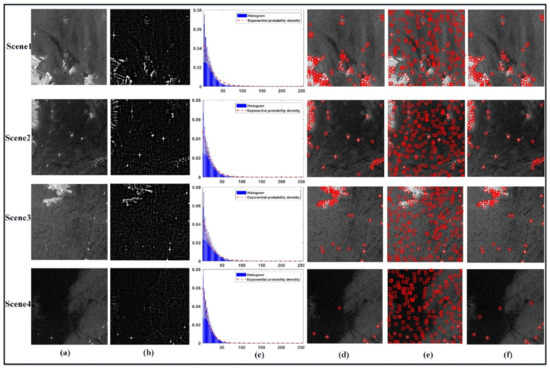
Figure 4.
Progress of candidate detection: (a) original image, (b) morphological process, (c) histogram and probability density function, (d) candidate detection by Otsu method, (e) candidate detection by constant false alarm rate (CFAR) (applying Gaussian distribution and the probability of false alarm is 0.0001), and (f) candidate detection by exponential inverse cumulative distribution function (EICDF).
Table 2.
Calculation of candidates and time.
2.4. Policies for Construction of Ship Detection Dataset
As a result of data pre-processing in Section 2.2, all targets contain false alarms and ships can be detected by ELCDF from the sub-images of No. 2 and No. 3, as shown in Figure 4f. Figure 5 presents the details of the false alarm and ship slices. For most of the ship slices, the backscatter intensity is relatively larger than the false alarms, and the rest are dark sea surface pixels distributed in the edges and corners. By contrast, the false alarm slices vary widely, some targets have strong backscatter intensity and the other has relatively weak backscatter intensity.
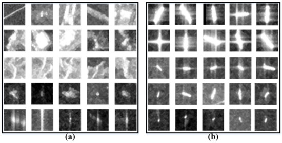
Figure 5.
Candidate target: (a) false alarm and (b) ships.
A dataset including both false alarm slices and ship slices is constructed to make the CNN model more robust in the training stage. The policies of the dataset construction are considering both ships of different sizes and non-ship objects with a very similar shape and structure to that of a ship. Hence, we divide both the ship and false alarm slices into different categories, and the detailed categories are listed as follow:
The false alarms are divided into four categories:
False alarm #1: The characteristics of this type of false alarm mainly come from artificial targets such as cross-sea bridges, tall buildings, lighthouses and others, which are similar to the ship slices, as shown in the first two rows in Figure 5a. Most of these targets have strong scattering intensity across the center.
False alarm #2: The characteristics of this type of false alarm mainly come from the land targets, where has a bright ridge line as shown in the third row of Figure 5a.
False alarm #3: The characteristics of this type of false alarm mainly come from natural targets such as small islands, reefs, and rocks, as shown in the fourth row of Figure 5a. Most of those targets are similar to the medium-level ship in the third row of Figure 5b, which has low scattering intensity across the center and is surrounded by a dark sea surface.
False alarm #4: The characteristics of this type of false alarm mainly come from azimuth ambiguity as explained in [37], which usually brings a great challenge in ship detection through the traditional method. This type of false alarm is distributed at the center of the slice, close to the backscattering intensity of the ships, as shown in the fifth row of Figure 5a.
The ships are divided into three categories:
Ship #1: The characteristics of these ships have a strong scattering intensity and a large-level size, as shown in the first two rows in Figure 5b.
Ship #2: The characteristics of these ships have a strong scattering intensity and a medium-level size, as shown in the third and fourth row in Figure 5b.
Ship #3: The characteristics of these ships have a low scattering intensity and a small-level size, which is similar to the ghost, as shown in the fifth row of Figure 5a,b.
After the pre-process and candidate detection by the VH and VV polarizations of No. 2 and No. 3 SAR images, then, labeled the false alarm and ship by comparing manually the SAR image and the Google Earth high-resolution optical image, and by considering the scattering characteristics and context information of targets. The results of a dataset of the ship and false alarms are listed in Table 3. VH and VH polarization have a total of 4198 false alarm slices and 3132 ship slices.
Table 3.
Pre-process detection result.
2.5. CNN Model
As mentioned, the classic object detectors tend to have deep convolutional layers and more training parameters, which often take a long time to train. In this letter, we introduce a two-layer lightweight CNN model similar to the classic LeNet-5 model [38], called the modified LeNet-5 (M-LeNet). Detailed information on the proposed CNN model is listed in Table 4. The CNN model contains convolution, MaxPool, rectified linear units (ReLU), dropout, and full-connection layers.
Table 4.
Details of M-LeNet model.
In general, the convolution operation computes its output as a nonlinear function of the weighted sum of its inputs and of a bias term θ, as shown in Equation (1).
In the previous studies, the input size was set to 60 × 60, 64 × 64, and 128 × 128, respectively [26,30,31,39]. In this letter, the input size was set to 32 × 32 to reduce the calculation and simplify the model. As the length and width of some marine objects in this study were larger than 32 pixels, the resize process was applied in the pre-process stage to ensure the same input size. To limit the number of weights to learn, all the filter kernels were set to 3 × 3. In the beginning, 16 convolutional kernels of size work on the input images to extract features, after which the outputs are downsampled by max-pooling kernels with a size of 2 × 2. Then, the second convolutional layer filters the outputs of the first pooling layer with 32 filter kernels. Thereafter, the convolutional layers are downsampled by the second pooling layer to shrink the feature maps. Finally, three fully connected layers (FC1 with 512 output neurons, FC2 with 128 output neurons, and FC3 with 2 output neurons) take the outputs of the dropout layers as input, and then the softmax function is used to predict the labels of the targets after the final output vector. The strides of all the convolutional layers and all the pooling layers are set to 1 and 2, respectively. Furthermore, overfitting may occur easily when a neural network is trained on a small dataset. The dropout layer [27] is used for every max-pooling and fully connected layer to prevent overfitting and improve the performance of the neural network. Furthermore, rectified Linear Unit (ReLU) is used for every convolutional layer and fully connected layer to prevent a vanishing or exploding gradient. The mathematical derivation of the forward and backpropagation algorithm was proved and discussed in [40].
The cross-entropy loss function is used to minimize the error between the ground truth and the CNN prediction output, which can be written as follows:
where w is the trainable weight parameter, m represents the total number of training samples, and yi, xi refer to the true label and predicted label of the ith example, respectively.
3. Experimental Results and Analysis
For the comprehensive evaluation of the ship detection result using the proposed method, two sub-images of the No. 1 SAR image acquired on 23 June 2020 located in the East China Sea area were clipped, as shown in Figure 6a–d. The sizes of the two sub-images were 3791 × 2847 and 2589 × 1565. Besides, a sub-image of 4339 × 3258 was also clipped from the No.4 SAR image acquired on 13 February 2021, located in the Huanghai Sea area, as shown in Figure 7a,b. Figure 6 shows that the land and island contain sea areas in both regions. The azimuth ambiguities are often caused by the sampling of the Doppler spectrum at finite intervals of the pulse repetition frequency (PRF) due to the acquisition mode of two channels [37]. Thus, in the SAR images, a small amount of “ghost” appears around the ship in high-speed movement, but is not negligible in ship detection. Figure 6e,f shows the azimuth ambiguities caused by ships moving at high speed. In general, the scattering intensity of co-polarization (see Figure 6b,d) is higher than that of cross-polarization (see Figure 6a,b). Thus, the same targets may present different scattering intensity in VH and VV polarization. The characteristic of the target in VH polarization is less than that in VV polarization, especially for the small targets. In previous studies, the co-polarization data were also selected for ship detection. However, the VH polarization is less influenced by azimuth ambiguities. Thus, in PolSAR images, the azimuth ambiguity was usually suppressed by two cross-polarization channels [37]. However, in previous studies, the performance of ship detection by VH and VV polarization was less discussed. Thus, considering the characteristics of dual-polarization SAR in marine imaging, we utilized VH and VV to detect the ship using the CNN method. Figure 8 shows the candidate results of ship detection based on the method described in Section 2.3. The sub-image with complex background presents that all ships can be detected, and false alarm caused by land, island and azimuth ambiguity also can be detected. There are 122 true ships and 244 false alarm targets in the sub-images of No. 1 SAR image and 17 true ship and 137 false alarm targets in the sub-image of No. 4 SAR image. The ground truth can be obtained by using SAR expert knowledge interpretation and Google Earth in order to evaluate the performance of the proposed method in the next section. It should be noted that the interpretation of those ground truth is to identify false alarms by comparing the SAR image with the high-resolution optical image on Google Earth and then identifying the ship based on the scattering characteristics and context of the ship on the SAR image.
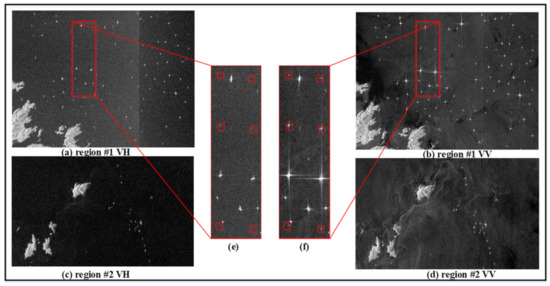
Figure 6.
Sub-images of No. 1 image vertical–horizontal (VH) and vertical–vertical (VV) polarizations in the East China Sea area. The red rectangle in (e,f) shows the azimuth ambiguities caused by ships in VH and VV polarization.
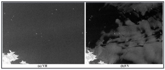
Figure 7.
Sub-images of No. 4 image VH and VV polarizations in the Huanghai Sea area.
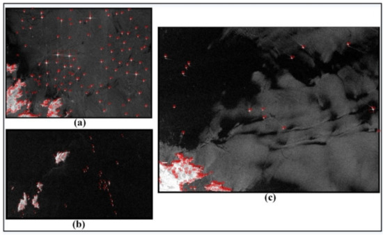
Figure 8.
Results of candidate detection. (a,b) The sub-image of the No. 1 SAR image located in the East China Sea area. (c) The sub-image of the No. 4 SAR image location in the Huanghai Sea area.
3.1. Training Details
In this section, the implementation of the hardware and platform is introduced in our experiments. We perform the experiments on the Ubuntu 14.04 operating system with an 11.9 GB memory NVIDIA TITAN Xp GPU. Inspired by the hyperparameters set of the literature [23,41,42], the learning rate, batch size, max epoch, moment, and momentum were set at 0.01, 32, 0.9, 1000, and 0.0005, respectively. Considering the SAR characteristics, we discarded the data augmentation in our experiment [43]. A set of optimal hyperparameters for a learning algorithm list in Table 5.
Table 5.
The hyperparameters settings.
To compare with our method, we also introduced machine-learning methods such as KNN, SVM, RF, and the classic CNN LeNet-5 method, which was commonly used and showed good performance in the classification task. In this letter, KNN, SVM, and random forest (RF) were implemented on the Ubuntu 14.04 operating system and Scikit-learn in Python. The parameters of KNN, SVM, and RF can be set with the default parameters. Besides, the classic CNN LeNet-5 method was also used. The hyperparameters of LeNet-5 were set as the M-LeNet. To ensure similarity in input data, these data were normalized to 0 and 1, with the values of mean and variance set to 0.5.
The training and validation samples are listed in Table 6. In all methods, the training and validation sample comes from 11 July 2020 (No. 2) and 23 July 2020 (No. 3), and the ratio is set at 8:2 in the training stage. In the testing stage, the test sample comes from the SAR data acquired on 23 June 2020 (No. 1) and 13 February 2021 (No. 4).
Table 6.
The information of training, validation, and test data.
3.2. VH Polarization Results
In this section, we first conducted the experiments on VH polarization by KNN, SVM, RF, LeNet-5, and our method. Figure 8 shows the candidate results of the ship and false alarm. Apart from the true ship, many false alarm targets are detected in the land and island areas. As mentioned above, in order to detect ships more accurately, a lightweight CNN method is proposed. Meanwhile, the KNN, SVM, RF, and classic LeNet-5 methods were introduced to indicate the effectiveness of our methods. Figure 9 shows the results of different methods through which all ships could be detected and false alarms were reduced further. The KNN method presents more false alarms and fewer true ships than the other methods. The performance of different machine learning methods was discussed [30,44]. Noi and Kappas [44] confirmed that when the number of training samples increases from 1267 pixels to 2619 pixels (each class has 135 polygons) in land cover classification experiments, the accuracy of SVM and RF is significantly better than that of KNN. Wang et al. [30] also demonstrated that the performance of KNN is less than that of RF and SVM in ship detection. Thus, the performance of RF and SVM is reasonably better than that of KNN. In the CNN method, the performance of M-LeNet is better than that of the LeNet-5 method.
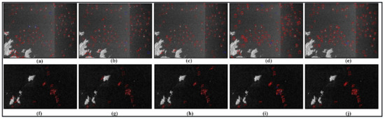
Figure 9.
Sub-image 1 (up) and sub-image 2 (down) detection results of VH polarization in the East China Sea area. (a–e) KNN, SVM, RF, LeNet-5, and M-LeNet, respectively. (f–j) KNN, SVM, RF, LeNet-5, and M-LeNet, respectively. (Red rectangle: ship, red rectangular box with arrow: false alarm, and blue rectangle: missed ship).
To quantitatively evaluate the performance of KNN, SVM, RF, LeNet-5, and M-LeNet, we introduced the evaluation indicator, such as accuracy, precision, recall, and F1 score. In these evaluation indicators, the F1 score is the weighted average of precision and recall, and is usually more useful than accuracy. The equations are as follows:
where true positive (TP) means that the ships are correctly predicted, true negative (TN) means that the ships are predicted to be false alarms, false positive (FP) means that the actual class is a false alarm and the predicted class is the ship, and false negative (FN) means that the actual class is the ship but the predicted class is a false alarm. In the CNN, the input data are the slices, the output is the probability of ships and false alarms. Hence, the evaluation performance is based on the number of ships and false alarms. Then, the accuracy, precision, recall, and F1 score were evaluated based on ground truth and the number of predictions of the ship and false alarm slices.
In addition, the number of missed ships and the number of false alarms were also calculated. In the sub-images, 122 true ships were obtained through expert knowledge interpretation using the SAR scattering mechanism. Table 7 presents the detailed evaluation indicators. RF provides the best evaluation indicators compared with KNN and SVM for the machine learning method. M-LeNet presents the best evaluation indicators for the CNN method. The number of the least missed ship is one in the RF method, and the number of the most missed ship is five in the KNN method. The number of the least false alarms is zero in M-LeNet, and the number of the most false alarms is eleven. The false alarm mainly occurs in the land areas in the lower-left corner of the image, which shows a structure similar to a ship, with low surrounding background. Furthermore, the false alarms caused by azimuth ambiguity are also incorrectly detected. Compared with VV polarization, VH polarization has lower backscattering, especially for small targets. Thus, the poor performance of this type of ship fails to be detected in the CNN methods, as indicated by the blue rectangles in Figure 9. The CNN method generally exhibits better performance than the machine learning method. Although several ships are missed, the overall performance of M-LeNet is better than that of RF. The reason is that the RF classifier based on the statistical model is sensitive to the image pixels, while the convolution and pooling kernel operations lead to the small targets miss detailed texture information and rich semantic information in the CNN method. Thus, the performance of small target detection in RF is better than that of M-LeNet and the performance of false alarm detection in M-LeNet is better than that of RF. Although the number of correct ship detections by M-LeNet is not as much as that of RF, the false number of ship detections is less than that of RF and LeNet-5. The comprehensive evaluation indicators such as the F1 score, accuracy, and recall show better performance than RF. M-LeNet showed the best performance with an F1 score of 0.99 and an accuracy of 99.40%. Besides, in order to show our CNN model more transferability, a SAR image located in the Huanghai Sea area was used to test the performance of ship detection. In order to quickly evaluate the accuracy, a sub-image with the size of 4339 × 3258 was clipped. In the sub-images, 17 true ships were obtained through expert knowledge interpretation and Google Earth. Although the number of the ship is less than the sub-images in No. 1, the VH and VV polarization shows different sea background. Figure 10 shows the detection results and Table 8 presents the detailed evaluation indicators. The LeNet-5 presents better performance than KNN, SVM, and RF with an F1 score of 0.90 and an accuracy of 98.05%. The M-LeNet shows the best performance in those methods with an F1 score of 0.97 and an accuracy of 99.35%.
Table 7.
Detailed evaluation index of VH polarization in the East China Sea area.
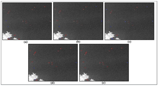
Figure 10.
Sub-image detection results of VH polarization in the Huanghai Sea. (a–e) represent KNN, SVM, RF, LeNet-5, and M-LeNet, respectively. (Red rectangle: ship, red rectangular box with arrow: false alarm, and blue rectangle: missed ship).
Table 8.
Detailed evaluation index of VH polarization in the Huanghai Sea area.
3.3. VV Polarization Results
Figure 11 shows the detection results of VV polarization. Similar to VH polarization, the more false alarms were reduced, the more ships were retained. In sub-image 1, the more false alarms mainly appeared in Figure 11a,b,d. In sub-image 2, the false alarms mainly existed in Figure 11f,g. Figure 11 shows that RF performs best in machine learning and M-LeNet performs best in deep learning. To quantitatively compare the performance of different methods, we calculated the accuracy, precision, recall, and F1 score. Table 9 presents the results of the evaluation indicators. The number of the least missed ship is zero in the RF and SVM method, and the number of the most missed ship is ten in the LeNet-5 method. The number of the least false alarms is three in M-LeNet, and the number of the most false alarms is twenty-one in the KNN method. RF and SVM could detect all the true ships, but a few false alarms were retained compared with VH polarization. Similar to the performance of VH polarization, KNN had more missed ships and false alarms. LeNet-5 performed worst with more missed ships. Although the number of missed ships in the M-LeNet method was more than that of RF and SVM, the comprehensive evaluation indicators showed the best performance with an F1 score of 0.98 and an accuracy of 98.2%. The characteristics of false alarms caused by azimuth ambiguity are similar to those of the true ship, so distinguishing the false alarms is difficult. Although the M-LeNet method could reduce false alarms caused by azimuth ambiguity more effectively than other methods, the false alarms still existed. In [31], 680 ships and 170 ghosts were selected for training; the experiments on the Sentinel-1 images showed encouraging results, but further improvement is needed. In our experiment, the number of ghosts was under 0.2%, which indicated a great imbalance for ship and ghost training samples. Thus, the predicted performance for the ghost is poor. Figure 12 shows the detection result and Table 10 presents the evaluation index of VV polarization in the No.4 sub-image of the Huanghai Sea area. Different from the VH polarization in Figure 10, the VV polarization image shows an inhomogeneous pattern in the SAR scene due to other marine phenomena that may exist in the images, e.g., moderate-to-high wind, upwelling, and eddies [45,46]. In those methods, the RF shows the better performance with an F1 score of 0.97 and an accuracy of 99.35% than other methods. Although the M-LeNet achieves an F1 score of 0.92 and an accuracy of 98.05%, the M-LeNet enables all ships detected in the inhomogeneous.
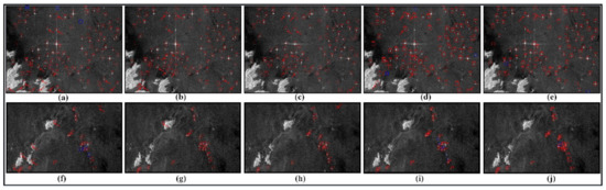
Figure 11.
Sub-image 1 (up) and sub-image 2 (down) detection results of VV polarization in the East China Sea area: (a–e) show KNN, SVM, RF, LeNet-5, and M-LeNet, respectively. (f–j) represent KNN, SVM, RF, LeNet-5, and M-LeNet, respectively. (Red rectangle: ship, red rectangular box with arrow: false alarm, and blue rectangle: missed ship).
Table 9.
Detailed evaluation index of VV polarization in the East China Sea area.
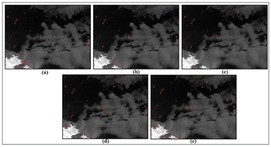
Figure 12.
Sub-image detection results of VV polarization in the Huanghai Sea area. (a–e) represent KNN, SVM, RF, LeNet-5, and M-LeNet, respectively. (Red rectangle: ship, red rectangular box with arrow: false alarm, and blue rectangle: missed ship).
Table 10.
Detailed evaluation index of VV polarization in the Huanghai Sea area.
3.4. CNN Feature Visualization Analysis
Deep neural networks have enabled unprecedented breakthroughs in classification, semantic segmentation, and object detection task. Although those CNN networks enable superior performance, interpreting and visualizing them are difficult due to the lack of decomposability into intuitive and understandable components [47]. CAM was proposed to identify discriminative regions by a restricted class of image classifications and to gain a better understanding of a model. However, any fully connected layer of the model was removed, and instead of global average pooling (GAP) to obtain the localization of a class [48]. Thus, altering the model architecture was unavoidable, training is needed again, and the available staffing scenarios are restricted. Grad-CAM improved the CAM by using the gradient information flowing into the last convolutional layer of CNN to understand the importance of each neuron for a classification decision [49]. Similar to CAM, Grad-CAM uses the feature maps produced by the last convolutional layer of a CNN. In CAM, we weigh these feature maps using weights taken out of the last fully connected layer of the network. In Grad-CAM, we obtained neuron importance weight using (Equation (5)) calculated based on the global average pool, with the gradients over the height dimension (indexed by ) and the width dimension (indexed by ). Therefore, Grad-CAM obtained the class discriminative localization map without a particular model architecture because we can calculate gradients through any kind of neural network layer we want. performs a weighted combination of forward activation maps, and follows it by ReLU to obtain the final class discriminative saliency map, as shown in Equation (6).
where weight is the feature map of a target class. represents feature map . is the feature map of a convolutional layer, of height , and width for any class , is the feature map of a convolutional layer, i.e., . Detailed information can be found in [49].
The output of Grad-CAM is a “class-discriminative localization map,” i.e., a heatmap where the hot part corresponds to a particular class. Figure 13 and Figure 14 show the Grad-CAM visualization heatmap for “false alarm” and “ship” of VH and VV polarization, respectively. The heatmap represents the image region with the greatest attention from CNN for the correct prediction of images belonging to a particular class. Figure 13a and Figure 14a show great attention through the CNN prediction of images belonging to false alarms. These image slices belong to the same area of the VH and VV polarization, which contain buildings near the sea-land, small island, reef, and azimuth ambiguity. The heatmap of false alarms shows that the surrounding background was conducive to the false alarm recognition. The azimuth ambiguity presented different characteristics in VH and VV polarization; a similar phenomenon has been discussed in Section 3. Fortunately, the azimuth ambiguity could be observed in the first row in VH and VV polarization. The azimuth ambiguity scattering intensity in VV polarization was more obvious than that in VH polarization. Furthermore, the false alarm in VV polarization presented different characteristics. One focused on the surrounding background from the heatmap, and another focused on the azimuth ambiguity itself, which was why the azimuth ambiguity of false alarm could not predict better in polarization. Figure 13b and Figure 14b show great attention through the CNN prediction of images belonging to the ship. The different scale ships with high scattering intensity had an important contribution to ship recognition than the surrounding sea surface, which was different from the false alarm in the VH and VV polarization.
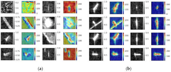
Figure 13.
Visualization of VH polarization: (a) heatmap of false alarm and (b) heatmap of ship.
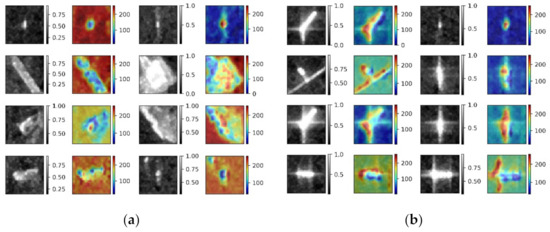
Figure 14.
Visualization of VV polarization: (a) heatmap of false alarm and (b) heatmap of ship.
4. Discussion
The performance of ship detection in CNN methods proves its great potential in different backgrounds such as incidence angles, wind speeds, sea states, and ocean dynamic parameters that mainly influence the backscattering coefficient between the ocean surface and the ship [23,50,51]. Besides, the scattering characteristics of ghosts caused by azimuth ambiguity when the ship is moving at high speed is similar to the characteristics of the ship, thereby causing difficulty in distinguishing between the ship and ghost in a single-polarization image. The CNN method also shows great potential. In this study, the performance of lightweight CNN does not completely suppress the ghost due to the lack of adequate training samples in VV polarization. Fortunately, the ghost in VH polarization is less affected, and thus, the performance of lightweight CNN shows the best result in VH polarization. Future work will be conducted to add the training samples of the ghost.
In the object detectors, the size of small targets is less than 32 × 32 for nature images [21]. However, the SAR images are different from the nature images, and the size of the ship is usually much less than 32 × 32, especially for ships operating offshore. Figure 15 shows the size of the ship in the test SAR image. Almost all ships have an area of less than 32 × 32, and most ships have an area of less than 24 × 25. The SVM and RF methods based on statistical characteristics show good performance with the fewest ships missed, especially the small ships in VV polarization; however, some false alarms cannot be avoided. The PFN module and feature fusion strategy are often used to improve the detection accuracy and reduce the false alarms of the small target [26,42,52]. Furthermore, those modules always integrate into the VGG16 and ResNet-50 networks [42,53]; the CNN models are complex and have many parameters to train. The PFN module and feature fusion strategy show effectiveness for small goals in object detectors, but may show poor effectiveness for much less than 32 × 32. Thus, in this study, we provide a dataset and two-stage method for ship detection with the SAR image, where even extremely small ships can be completely recognized in the first stage. In the second stage, the different scale candidates in the test SAR images can be accurately detected by considering context background information. The best and stable performance of ship detection is demonstrated by M-LeNet, which can reduce the false alarms and missed ships, and obtain higher precision in VH and VV polarization than other methods in different ocean areas and scenarios.
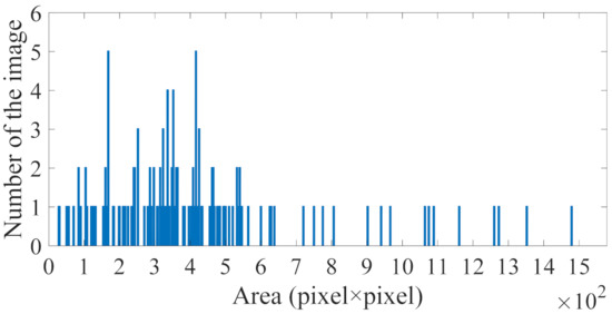
Figure 15.
Area of the ship in test data.
In the previous studies, the ship detection using sentinel-1 SAR images was carried out by Wang et al. [54]. The performance of ship detection can reach an accuracy of 98.07% and an F1 score of 0.90 by Faster RCNN, thus, the number of false alarms was detected to be relatively large [54]. The accuracy could reach 90.05% based on YOLOv2 for imagery [55]. The test precision and F1 score were 91.3% and 0.92 for detecting multiscale ships and small ships, when using the GF-3 dataset, respectively [42]. In [29], the attention module was used to improve the performance of ship detection, the recall, precision, and F1 score could reach 0.96, 96.4%, and 0.96, respectively. Although the performance of ship detection was improved, the model complexity had increased. To reduce model complexity, a simple CNN was used to detect the ship, and the accurate rate of ship detection was 97.2% when using the spaceborne image [30]. The lightweight CNN was proposed to improve the accuracy and F1 score in our experiments. The performance of lightweight CNN shows that the best result can reach an accuracy of 99.4% and an F1 score of 0.99 based on Sentinel-1 images. Figure 15 shows the most ship has an area of less than 24 × 25 pixel. The test accuracy and F1 score also demonstrate the proposed method can detect the small-level ship. To sum up, the proposed method can detect the ship effectively in contrast to that with the detector above. Unfortunately, it was rarely analyzed and visualized the feature to gain a better understanding of a model in the previous studies. In order to understand and visualize the model, the Grad-CAM was used, and the result demonstrated it could help us understand the mechanism of how the ship and false alarm was predicted by the lightweight CNN model work. Hence, based on the visualization and analysis of the Grad-CAM, it can be used to help to detect the ship with the weakly unsupervised method in future work.
From the above discussion, the lightweight CNN we proposed can show good performance in different ocean areas and scenarios. The difference with those detectors [29,54,55] does not need the input data and ground truth bounding box one-to-one correspondence, and only labeled in ship and no-ship. Besides, the CNN model we proposed is simplified as a shallow convolution neural network and improves efficiency in comparison with Faster RCNN, SSD, and Yolo, etc. However, comparing with those detectors, the CNN model we proposed is not end-to-end. To obtain the detect result, the data preprocess first needs to be applied to SAR images, then the lightweight CNN is used to accurately detect the ship. Although, the proposed method shows an accuracy of 99.4% and an F1 score of 0.99, how to simplify the data preprocess and integrate it into the CNN model to achieve end-to-end training is worth considering in future work. Besides, the ocean surface is modulated and complexed by ocean dynamics processes such as wind, waves, upwelling, and eddies, as well as sea state. Due to the limited data for training, it cannot cover all sea state conditions. The CNN model was not truly explored with comparably limited training data by Zhang et al. [5]. Hence, in order to make the CNN model to have more generalization capability, more data should be added in future work.
5. Summary and Conclusions
In this paper, the two-stage ship detection method is proposed in a complex background, i.e., in the offshore area. First, the SAR data pre-process contains the image filter, island filter, and threshold segmentation. The island filter is proposed to improve the ship contrast using a convolutional kernel, and threshold segmentation is proposed for slice production and candidate detection for time-saving. Second, the CNN model is proposed for slice fine classification and recognition. The experiment demonstrates that compared with the KNN, SVM, RF, and LeNet-5 methods, the proposed method can obtain stable accuracy in VH and VV polarization. Furthermore, although the proposed method cannot eliminate the false alarm caused by azimuth ambiguity in VV polarization because the few ghosts of false alarms sample in the training stage are insufficient to maintain the balance between the ship and false alarm, the false alarm caused by azimuth ambiguity in VH polarization give a little contribution. The detection performance shows better results in both VH and VV polarization for the ship size of much less than 32 × 32. Fortunately, the CNN interpretation and visualization of the ship and false alarm are accurate predictions through Grad-CAM visualized analysis. The experiments demonstrate that the high scattering intensity of the ship itself provides an important contribution to ship recognition rather than the surrounding sea surface in VH and VV polarization. However, the surrounding sea surface is useful for false alarm recognition in VH and VV polarization.
Author Contributions
Conceptualization, J.Z. and W.S.; data curation, L.Z.; methodology, X.G. and L.S.; supervision, P.L. and J.Y.; validation, X.G.; writing—original draft, X.G.; writing—review and editing, X.G. All authors have read and agreed to the published version of the manuscript.
Funding
This study was funded by the National Natural Science Foundation of China under Grant Nos. 42071295, 41771377 and 41901286. The Key Laboratory of Surveying and Mapping Science and Geospatial Information Technology of Ministry of Natural Resources under Grant No. 201906, and the Open Research Fund of Jiangsu Key Laboratory of Resources and Environmental Information Engineering, CUMT under Grant No. JS201909.
Acknowledgments
The authors are grateful to the Hubei Province Postdoctoral Science and Technology Preferred Project for funding this study. They thank the European Space Agency and Alaska Satellite Facility for providing free Sentinel-1 data online. The authors would also like to thank the anonymous reviewers for their comments to improve this article.
Conflicts of Interest
The authors declare no conflict of interest.
References
- Ai, J.; Qi, X.; Yu, W.; Deng, Y.; Liu, F.; Shi, L. A New CFAR Ship Detection Algorithm Based on 2-D Joint Log-Normal Distribution in SAR Images. IEEE Geosci. Remote Sens. Lett. 2010, 7, 806–810. [Google Scholar] [CrossRef]
- Ai, J.-Q.; Qi, X.-Y.; Yu, W.-D. Improved Two Parameter CFAR Ship Detection Algorithm in SAR Images. J. Electron. Inf. Technol. 2009, 31, 2881–2885. [Google Scholar]
- Dai, H.; Du, L.; Wang, Y.; Wang, Z. A Modified CFAR Algorithm Based on Object Proposals for Ship Target Detection in SAR Images. IEEE Geosci. Remote Sens. Lett. 2016, 13, 1925–1929. [Google Scholar] [CrossRef]
- Wang, C.; Bi, F.; Zhang, W.; Chen, L. An Intensity-Space Domain CFAR Method for Ship Detection in HR SAR Images. IEEE Geosci. Remote Sens. Lett. 2017, 14, 529–533. [Google Scholar] [CrossRef]
- Zhang, W.; Liljedahl, A.K.; Kanevskiy, M.; Epstein, H.E.; Jones, B.M.; Jorgenson, M.T.; Kent, K. Transferability of the deep learning mask R-CNN model for automated mapping of ice-wedge polygons in high-resolution satellite and UAV images. Remote Sens. 2020, 12, 1085. [Google Scholar] [CrossRef]
- Bhuiyan, M.A.E.; Witharana, C.; Liljedahl, A.K. Use of Very High Spatial Resolution Commercial Satellite Imagery and Deep Learning to Automatically Map Ice-Wedge Polygons across Tundra Vegetation Types. J. Imaging 2020, 6, 137. [Google Scholar] [CrossRef]
- Yang, W.; Zhang, X.; Luo, P. Transferability of Convolutional Neural Network Models for Identifying Damaged Buildings Due to Earthquake. Remote Sens. 2021, 13, 504. [Google Scholar] [CrossRef]
- Zhang, C.; Wei, S.; Ji, S.; Lu, M. Detecting Large-Scale Urban Land Cover Changes from Very High Resolution Remote Sensing Images Using CNN-Based Classification. ISPRS Int. J. Geo-Inf. 2019, 8, 189. [Google Scholar] [CrossRef]
- Wang, Y.-R.; Li, X.-M. Arctic sea ice cover data from spaceborne SAR by deep learning. Earth Syst. Sci. Data Discuss. 2020, 1–30. [Google Scholar] [CrossRef]
- Shao, Z.; Zhou, W.; Deng, X.; Zhang, M.; Cheng, Q. Multilabel Remote Sensing Image Retrieval Based on Fully Convolutional Network. IEEE J. Sel. Top. Appl. Earth Obs. Remote Sens. 2020, 13, 318–328. [Google Scholar] [CrossRef]
- Girshick, R.; Donahue, J.; Darrell, T.; Malik, J. Region-based convolutional networks for accurate object detection and segmentation. IEEE Trans. Pattern Anal. Mach. Intell. 2015, 38, 142–158. [Google Scholar] [CrossRef] [PubMed]
- Girshick, R. Fast r-cnn. In Proceedings of the IEEE International Conference on Computer Vision, Santiago, Chile, 7–13 December 2015; pp. 1440–1448. [Google Scholar]
- Ren, S.; He, K.; Girshick, R.; Sun, J. Faster r-cnn: Towards real-time object detection with region proposal networks. In Proceedings of the Advances in Neural Information Processing Systems, Barcelona, Spain, 5–10 December 2016; pp. 91–99. [Google Scholar]
- Liu, W.; Anguelov, D.; Erhan, D.; Szegedy, C.; Reed, S.; Fu, C.-Y.; Berg, A.C. Ssd: Single shot multibox detector. In Proceedings of the European Conference on Computer Vision, Amsterdam, The Netherlands, 8–16 October 2016; pp. 21–37. [Google Scholar]
- Redmon, J.; Farhadi, A. Yolov3: An incremental improvement. arXiv 2018, arXiv:1804.02767. [Google Scholar]
- Redmon, J.; Farhadi, A. YOLO9000: Better, faster, stronger. In Proceedings of the IEEE Conference on Computer Vision and Pattern Recognition, Honolulu, HI, USA, 21–26 July 2017; pp. 7263–7271. [Google Scholar]
- Bochkovskiy, A.; Wang, C.-Y.; Liao, H.-Y.M. YOLOv4: Optimal Speed and Accuracy of Object Detection. arXiv 2020, arXiv:2004.10934. [Google Scholar]
- Redmon, J.; Divvala, S.; Girshick, R.; Farhadi, A. You only look once: Unified, real-time object detection. In Proceedings of the IEEE Conference on Computer Vision and Pattern Recognition, Las Vegas, NV, USA, 27–30 June 2016; pp. 779–788. [Google Scholar]
- Lin, T.-Y.; Goyal, P.; Girshick, R.; He, K.; Dollár, P. Focal loss for dense object detection. In Proceedings of the IEEE International Conference on Computer Vision, Venice, Italy, 22–29 October 2017; pp. 2980–2988. [Google Scholar]
- Everingham, M.; Van Gool, L.; Williams, C.K.; Winn, J.; Zisserman, A. The pascal visual object classes (voc) challenge. Int. J. Comput. Vis. 2010, 88, 303–338. [Google Scholar] [CrossRef]
- Lin, T.-Y.; Maire, M.; Belongie, S.; Hays, J.; Perona, P.; Ramanan, D.; Dollár, P.; Zitnick, C.L. Microsoft coco: Common objects in context. In Proceedings of the European Conference on Computer Vision, Zurich, Switzerland, 6–12 September 2014; pp. 740–755. [Google Scholar]
- Li, J.; Qu, C.; Shao, J. Ship detection in SAR images based on an improved faster R-CNN. In Proceedings of the Sar in Big Data Era: Models, Methods & Applications, Beijing, China, 13–14 November 2017. [Google Scholar]
- Wang, Y.; Wang, C.; Zhang, H.; Dong, Y.; Wei, S. A SAR dataset of ship detection for deep learning under complex backgrounds. Remote Sens. 2019, 11, 765. [Google Scholar] [CrossRef]
- Li, B.; Liu, B.; Huang, L.; Guo, W.; Zhang, Z.; Yu, W. OpenSARShip 2.0: A large-volume dataset for deeper interpretation of ship targets in Sentinel-1 imagery. In Proceedings of the 2017 SAR in Big Data Era: Models, Methods and Applications (BIGSARDATA), Beijing, China, 13–14 November 2017; pp. 1–5. [Google Scholar]
- Wei, S.; Zeng, X.; Qu, Q.; Wang, M.; Su, H.; Shi, J. HRSID: A high-resolution SAR images dataset for ship detection and instance segmentation. IEEE Access 2020, 8, 120234–120254. [Google Scholar] [CrossRef]
- Ma, M.; Chen, J.; Liu, W.; Yang, W. Ship Classification and Detection Based on CNN Using GF-3 SAR Images. Remote Sens. 2018, 10, 2043. [Google Scholar] [CrossRef]
- Krizhevsky, A.; Sutskever, I.; Hinton, G.E. Imagenet classification with deep convolutional neural networks. Commun. ACM 2017, 60, 84–90. [Google Scholar] [CrossRef]
- Zhang, T.; Zhang, X. High-Speed Ship Detection in SAR Images Based on a Grid Convolutional Neural Network. Remote Sens. 2019, 11, 1206. [Google Scholar] [CrossRef]
- Zhao, Y.; Zhao, L.; Xiong, B.; Kuang, G. Attention receptive pyramid network for ship detection in SAR images. IEEE J. Sel. Top. Appl. Earth Obs. Remote Sens. 2020, 13, 2738–2756. [Google Scholar] [CrossRef]
- Wang, Z.; Yang, T.; Zhang, H. Land contained sea area ship detection using spaceborne image. Pattern Recognit. Lett. 2020, 130, 125–131. [Google Scholar] [CrossRef]
- Cozzolino, D.; Di Martino, G.; Poggi, G.; Verdoliva, L. A fully convolutional neural network for low-complexity single-stage ship detection in Sentinel-1 SAR images. In Proceedings of the 2017 IEEE International Geoscience and Remote Sensing Symposium (IGARSS), Fort Worth, TX, USA, 23–28 July 2017; pp. 886–889. [Google Scholar]
- Martinez, W.L.; Martinez, A.R. Computational Statistics Handbook with MATLAB; CRC Press: Boca Raton, FL, USA, 2015; Volume 22. [Google Scholar]
- Davis, T.A. MATLAB Primer; CRC Press: Boca Raton, FL, USA, 2010. [Google Scholar]
- Lee, J.S.; Grunes, M.R.; De Grandi, G. Polarimetric SAR speckle filtering and its implication for classification. IEEE Trans. Geosci. Remote Sens. 2002, 37, 2363–2373. [Google Scholar]
- Wang, Z.; Wang, C.; Zhang, H.; Wang, F.; Jin, F.; Xie, L. SAR-based ship detection in sea areas containing small islands. In Proceedings of the 2015 IEEE 5th Asia-Pacific Conference on Synthetic Aperture Radar (APSAR), Singapore, 1–4 September 2015; pp. 591–595. [Google Scholar]
- Xu, X.; Xu, S.; Jin, L.; Song, E. Characteristic analysis of Otsu threshold and its applications. Pattern Recognit. Lett. 2011, 32, 956–961. [Google Scholar] [CrossRef]
- Velotto, D.; Soccorsi, M.; Lehner, S. Azimuth ambiguities removal for ship detection using full polarimetric X-band SAR data. IEEE Trans. Geosci. Remote Sens. 2013, 52, 76–88. [Google Scholar] [CrossRef]
- El-Sawy, A.; Hazem, E.-B.; Loey, M. CNN for handwritten arabic digits recognition based on LeNet-5. In Proceedings of the International Conference on Advanced Intelligent Systems and Informatics, Cairo, Egypt, 24–26 October 2016; pp. 566–575. [Google Scholar]
- Sharifzadeh, F.; Akbarizadeh, G.; Kavian, Y.S. Ship Classification in SAR Images Using a New Hybrid CNN-MLP Classifier. J. Indian Soc. Remote Sens. 2019, 47, 551–562. [Google Scholar] [CrossRef]
- Wu, J. Introduction to convolutional neural networks. Natl. Key Lab Nov. Softw. Technol. Nanjing Univ. China 2017, 5, 23. [Google Scholar]
- Kim, K.; Hong, S.; Choi, B.; Kim, E. Probabilistic Ship Detection and Classification Using Deep Learning. Appl. Sci. 2018, 8, 936. [Google Scholar] [CrossRef]
- Dai, W.; Mao, Y.; Yuan, R.; Liu, Y.; Pu, X.; Li, C. A Novel Detector Based on Convolution Neural Networks for Multiscale SAR Ship Detection in Complex Background. Sensors 2020, 20, 2547. [Google Scholar] [CrossRef]
- Goodfellow, I.; Bengio, Y.; Courville, A. Deep Learning; Mit Press: Cambridge, MA, USA, 2016. [Google Scholar]
- Thanh Noi, P.; Kappas, M. Comparison of Random Forest, k-Nearest Neighbor, and Support Vector Machine Classifiers for Land Cover Classification Using Sentinel-2 Imagery. Sensors 2018, 18, 18. [Google Scholar] [CrossRef]
- Zhu, S.; Shao, W.; Armando, M.; Shi, J.; Sun, J.; Yuan, X.; Hu, J.; Yang, D.; Zuo, J. Evaluation of Chinese quad-polarization Gaofen-3 SAR wave mode data for significant wave height retrieval. Can. J. Remote Sens. 2018, 44, 588–600. [Google Scholar] [CrossRef]
- Corcione, V.; Grieco, G.; Portabella, M.; Nunziata, F.; Migliaccio, M. A novel azimuth cutoff implementation to retrieve sea surface wind speed from SAR imagery. IEEE Trans. Geosci. Remote Sens. 2018, 57, 3331–3340. [Google Scholar] [CrossRef]
- Lipton, Z.C. The mythos of model interpretability. Queue 2018, 16, 31–57. [Google Scholar] [CrossRef]
- Lin, M.; Chen, Q.; Yan, S. Network in network. arXiv 2013, arXiv:1312.4400. [Google Scholar]
- Selvaraju, R.R.; Cogswell, M.; Das, A.; Vedantam, R.; Parikh, D.; Batra, D. Grad-cam: Visual explanations from deep networks via gradient-based localization. In Proceedings of the IEEE International Conference on Computer Vision, Venice, Italy, 22–29 October 2017; pp. 618–626. [Google Scholar]
- Tings, B.R.; Bentes, C.; Velotto, D.; Voinov, S. Modelling ship detectability depending on TerraSAR-X-derived metocean parameters. Ceas Space J. 2019, 11, 81–94. [Google Scholar] [CrossRef]
- Wang, Y.; Wang, C.; Zhang, H.; Dong, Y.; Wei, S. Automatic Ship Detection Based on RetinaNet Using Multi-Resolution Gaofen-3 Imagery. Remote Sens. 2019, 11, 531. [Google Scholar] [CrossRef]
- Zhang, G.; Li, Z.; Li, X.; Yin, C.; Shi, Z. A Novel Salient Feature Fusion Method for Ship Detection in Synthetic Aperture Radar Images. IEEE Access 2020, 8, 215904–215914. [Google Scholar] [CrossRef]
- He, J.; Guo, Y.; Yuan, H. Ship Target Automatic Detection Based on Hypercomplex Flourier Transform Saliency Model in High Spatial Resolution Remote-Sensing Images. Sensors 2020, 20, 2536. [Google Scholar] [CrossRef]
- Wang, Y.; Wang, C.; Zhang, H. Combining a single shot multibox detector with transfer learning for ship detection using sentinel-1 SAR images. Remote Sens. Lett. 2018, 9, 780–788. [Google Scholar] [CrossRef]
- Chang, Y.-L.; Anagaw, A.; Chang, L.; Wang, Y.C.; Hsiao, C.-Y.; Lee, W.-H. Ship Detection Based on YOLOv2 for SAR Imagery. Remote Sens. 2019, 11, 786. [Google Scholar] [CrossRef]


Publisher’s Note: MDPI stays neutral with regard to jurisdictional claims in published maps and institutional affiliations. |
© 2021 by the authors. Licensee MDPI, Basel, Switzerland. This article is an open access article distributed under the terms and conditions of the Creative Commons Attribution (CC BY) license (http://creativecommons.org/licenses/by/4.0/).