Abstract
Land surface temperature (LST) is a critical parameter of surface energy fluxes and has become the focus of numerous studies. LST downscaling is an effective technique for supplementing the limitations of the coarse-resolution LST data. However, the relationship between LST and other land surface parameters tends to be nonlinear and spatially nonstationary, due to spatial heterogeneity. Nonlinearity and spatial nonstationarity have not been considered simultaneously in previous studies. To address this issue, we propose a multi-factor geographically weighted machine learning (MFGWML) algorithm. MFGWML utilizes three excellent machine learning (ML) algorithms, namely extreme gradient boosting (XGBoost), multivariate adaptive regression splines (MARS), and Bayesian ridge regression (BRR), as base learners to capture the nonlinear relationships. MFGWML uses geographically weighted regression (GWR), which allows for spatial nonstationarity, to fuse the three base learners’ predictions. This paper downscales the 30 m LST data retrieved from Landsat 8 images to 10 m LST data mainly based on Sentinel-2A images. The results show that MFGWML outperforms two classic algorithms, namely thermal image sharpening (TsHARP) and the high-resolution urban thermal sharpener (HUTS). We conclude that MFGWML combines the advantages of multiple regression, ML, and GWR, to capture the local heterogeneity and obtain reliable and robust downscaled LST data.
1. Introduction
Land surface temperature (LST) refers to the radiative temperature of the Earth’s surface. LST is highly responsive to the interactions between the land surface and the atmosphere, water circulation, and energy exchange from the local scale to the global scale [1]. Therefore, LST is an essential parameter in various environmental research fields, including climate change and urban heat island effect monitoring [2,3]; land-surface carbon, water, energy, and evapotranspiration mapping [4,5]; soil moisture condition and drought assessment [6,7]; and forest fire detection [8]. Accurate LST measurements at different scales can facilitate these environmental monitoring studies.
Obtaining LST data over extensive areas via ground measurement is impractical, but the advent of satellite-based thermal infrared (TIR) sensors addresses this issue [1]. However, there is a trade-off between the spatial resolution and temporal resolution of TIR data [9]. Some sensors, such as the Moderate Resolution Imaging Spectroradiometer (MODIS), provide TIR images with high temporal resolutions (one day or less) but coarse spatial resolutions (1 km). Conversely, some sensors, such as the Advanced Spaceborne Thermal Emission Reflection Radiometer (ASTER), provide TIR images with relatively high spatial resolutions (300 m) but relatively coarse temporal resolutions (15 days). Moreover, thermal pixels inevitably contain multiple anisothermal objects, known as the thermal mixture effect [9]. These issues seriously impede LST applications. Hence, enhancing the spatial resolutions of LST products is increasingly urgent [9].
Spatial downscaling of LST is a widely adopted approach to enhance the spatial resolutions of LST products [9]. Current LST downscaling methods are categorized as physical mechanism-based models and statistics-based models [10]. Physical mechanism-based models aim to establish a physically meaningful relationship between thermal radiance (or LST) and ancillary data (such as land-cover maps) based on the principle of thermal radiation. Classic physical mechanism-based models include pixel block intensity modulation (PBIM) [11] and emissivity modulation (EM) models [12]. Guo and Moore (1998) [11] proposed PBIM to integrate the topographic spatial details recorded in Landsat TM reflective spectral images (30 m) into each thermal pixel block of the TM thermal image (120 m). However, PBIM is not applicable to very flat areas and nighttime images [11]. To downscale nighttime thermal images, Nichol (2009) [12] developed the EM algorithm. In addition to these modulation-based models, Liu and Pu (2008) [13] developed a new physical model (PM) based on spectral mixture analyses, and then Liu and Zhu (2012) [14] proposed the enhanced PM (EPM). Physical mechanism-based models are conducive to the scientific interpretation of the results, but their implementation complexity limits their applications.
Compared with physical mechanism-based models, statistics-based models are easier to implement and have become popular. Statistics-based models are established based on the statistical relationships between LST and other land surface parameters extracted from ancillary data with relatively high spatial resolutions. Typical ancillary data include the reflectance data of visible, near-infrared (NIR), and shortwave infrared (SWIR) bands, digital elevation model (DEM) data, and land-cover maps. Classic statistics-based downscaling models involve disaggregation procedure for radiometric surface temperature (DisTrad) [15], thermal image sharpening (TsHARP) [16], and high-resolution urban thermal sharpener (HUTS) [17]. Kustas et al. (2003) [15] assumed that a unique scale-independent relationship between the radiometric surface temperature () and the vegetation index (VI) exists within a sensor scene and proposed the DisTrad algorithm, using the normalized difference vegetation index (NDVI) as the scale factor. Agam et al. (2007) [16] modified the DisTrad algorithm by replacing the NDVI with fractional vegetation cover (FVC) to develop the TsHARP algorithm. However, the “” relationship is only suitable for LST downscaling in homogeneous vegetated areas. It cannot be applied to explain all the LST variations in urban areas or other non-vegetated regions, such as arid areas. Moreover, it varies easily with the seasons. Therefore, many other important determinants of LST have been introduced for LST downscaling. For example, Essa et al. (2012) [18] adapted the DisTrad algorithm by replacing the NDVI with an impervious percentage index, which is less affected by seasonal changes and more stable than the NDVI. Pan et al. (2018) [10] proposed the normalized difference sand index (NDSI) for LST downscaling in arid regions. Single-factor models are simple, but applying one indicator is inadequate for sufficiently describing LST. Therefore, some researchers employed two different indicators as scale factors. For instance, Dominguez et al. (2011) [17] integrated the NDVI and surface albedo to develop the HUTS algorithm. Duan et al. (2016) [19] and Bartkowiak et al. (2019) [20] adopted the NDVI and DEM data as scale factors to implement LST downscaling. Zhang et al. (2019) [21] combined the temperature and vegetation dryness index (TVDI) with DEM to downscale MODIS LST from 1000 to 90 m. Previous studies have shown that the two-factor models performed significantly better than TsHARP [17,19].
However, the two-factor models are still inadequate as LST heterogeneity is related to several types of environmental factors, such as land cover, topography, soil moisture, incoming solar radiation, and wind speed [1]. Recent studies have indicated that multiple indices should be integrated to improve LST downscaling accuracies [22,23]. For example, Zakšek and Oštir (2012) [22] selected the NDVI, enhanced vegetation index (EVI), albedo, emissivity, land-cover data, DEM, slope, aspect, and sky-view factor as the input parameters of a linear LST downscaling model. Yang et al. (2017) [23] developed a linear multiscale-factor downscaling approach that is based on an adaptive threshold, which involved the soil-adjusted vegetation index (SAVI), normalized multiband drought index (NMDI), modified normalized difference water index (MNDWI), and normalized difference built-up index (NDBI). However, the relationship between LST and multiple indicators tends to be nonlinear, and linear models are usually incapable of representing nonlinear relationships. To address this issue, researchers have introduced many machine learning (ML) algorithms for LST downscaling, such as random forest (RF) [24,25,26,27], extreme learning machine (ELM) [25], artificial neural networks (ANN) [26], support vector machine (SVM) [25,26,28], gradient boosting machine (GBM) [28], partial least squares (PLS) [28], and multivariate adaptive regression spline (MARS) [29]. For example, Hutengs and Vohland (2016) [24] applied the RF to LST downscaling for the first time and demonstrated that it was effective. Yang et al. (2017) [27] utilized the RF to downscale LST in an arid area with multiple remote sensing indices. Ebrahimy and Azadbakht (2019) [25] compared the RF, SVM, and ELM for the spatial downscaling of MODIS LST data, and the results showed that the RF and ELM outperformed the SVM. Li et al. (2019) [26] compared the RF, ANN, and SVM to downscale MODIS LST data and concluded that the RF and ANN performed better than the SVM.
However, these methods are global models, and their predictions may be locally misleading due to the local heterogeneity of LST and other land surface parameters [30]. A global model assumes that the relationship between the dependent and explanatory variables is stationary (i.e., does not vary) in space. However, LST and other land surface parameters are geographical variables; their relationships vary across space. This spatial characteristic is referred to as spatial nonstationarity (i.e., instability) [30], which contradicts the assumption of global models. Therefore, many researchers have focused on fitting the local relationships between LST and auxiliary parameters to improve the LST downscaling accuracy. Typical local statistical approaches include the moving window method and the method based on geographically weighted regression (GWR-based). The GWR-based method in this paper means GWR or a combination of GWR and other methods. For example, Zakšek and Oštir (2012) [22] locally adapted the multiple regression equation, using the moving window technique to downscale LST data. Gao et al. (2017) [31] proposed an indirect criterion based on aggregation-disaggregation (ICAD) to determine the optimal regression window for LST downscaling. Xia et al. (2019) [32] introduced the object-based window (OWS) method to downscale LST. Wu et al. (2019) [33] utilized GWR to build a nonstationary relationship between LST and the indicators for LST downscaling and concluded that GWR outperformed TsHARP. Yang et al. (2019) [34] integrated the multiscale GWR model with area-to-point kriging to downscale MODIS LST data. Peng et al. (2019) [35] proposed a geographically and temporally weighted regression (GTWR) model for LST downscaling over heterogeneous urban regions. Wang et al. (2020) [36] proposed a geographically weighted autoregressive (GWAR) model for spatial downscaling of MODIS LST. However, the GWR-based methods are also linear models, which are insufficient for simulating the nonlinear relationships between LST and multi-type indicators. Moreover, GWR is highly susceptible to the effects of multicollinearity, which leads to unreliable predictions when the explanatory variables are highly correlated [26].
Although researchers have made great efforts to improve the LST downscaling accuracy, most previous studies still have other limitations. First, multiple regression models are prone to overfitting, which is a common issue. Therefore, feature selection should be the first and most crucial step in the model design stage. However, the features selected in most multi-factor studies are not optimal for LST downscaling models as they disregard the correlations among features and the feature combination effects. In practice, highly correlated features are redundant, which will reduce the prediction performance and stability of models. More importantly, features act on a model in combination rather than individually [37]. Accordingly, researchers should pay more attention to obtaining the optimal feature combination for each LST downscaling model. Second, most previous LST downscaling studies involved MODIS LST, Landsat LST, and ASTER LST data but rarely employed high-resolution images without TIR bands, such as Sentinel-2A data. Sentinel-2A data have the advantages of relatively high resolutions (10 m) and open access. Therefore, LST downscaling based on Sentinel-2A data needs more investigations to obtain LST data with relatively high resolution. Third, most multi-factor LST downscaling studies utilized classic single-factor algorithms, such as DisTrad and TsHARP, as benchmarks. However, as mentioned above, LST heterogeneity is related to multi-type factors, so that a single factor (such as NDVI) is inadequate for representing LST. In terms of LST downscaling, the multi-factor models outperform the single-factor models is within expectation. Therefore, the model comparison between multi-factor models and the single-factor models is not sufficient. Model comparisons that use the two-factor algorithms or other multi-factor approaches as benchmarks need further investigation.
In this context, the objectives of this paper involve three aspects: (1) providing an objective feature selection scheme to select the optimal feature combination for each model; (2) developing a multi-factor geographically weighted machine learning (MFGWML) downscaling method, to produce reliable and robust 10 m LST data based on Sentinel-2A images; (3) assessing the MFGWML model by comparing it with two classic downscaling algorithms, namely the single-factor model (namely TsHARP) and the two-factor model (namely HUTS). The remainder of this paper is arranged as follows: Section 2 introduces the study area, data, and methods. Section 3 evaluates the LST downscaling results. Furthermore, Section 4 describes the limitations of this paper and future research. Section 5 summarizes the conclusions.
2. Materials and Methods
2.1. Study Area
Beijing (39°28′N–41°05′N, 115°25′E–117°30′E), the capital of China, is located in northern China (Figure 1) and covers an area of approximately 16,410.54 . The general topography of Beijing is high in the northwest and low in the southeast, and the average altitude is 43.5 . Beijing is located in a warm temperate zone, and its climate type is a typical semi-humid continental monsoon climate. Beijing is hot and rainy in summer, dry and cold in winter, and has short spring and autumn seasons. The monthly average temperatures in January and July are −3.7 and 26.2 °C, respectively. The annual average air temperature is approximately 12.3 °C. The annual precipitation in Beijing is 572 , and summer precipitation accounts for approximately 3/4 of the annual precipitation. With the acceleration of urbanization, the population of Beijing has rapidly increased. By the end of 2018, Beijing had a population of 21.542 million, and its urbanization rate was 86.5%.
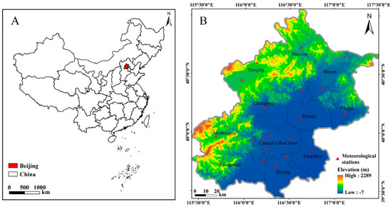
Figure 1.
Geographical location map of the study area. Panel (A) presents the location of Beijing in China. Panel (B) shows the spatial extent, elevation, locations of 20 national meteorological stations, and boundaries and names of the districts in Beijing.
2.2. Data Description and Image Preprocessing
The Landsat 8 L1TP products, Sentinel-2A Level-1C products, and Shuttle Radar Topography Mission (SRTM) data were downloaded from the United States Geological Survey (USGS) website (https://earthexplorer.usgs.gov/ (accessed on 17 March 2021)). Landsat 8 and Sentinel-2A images are both defined in the Universal Transverse Mercator (UTM) map projection with the World Geodetic System 84 (WGS84) datum. As shown in Table 1, their corresponding bands have almost consistent spectral ranges. Three Landsat 8 images and seven Sentinel-2A images are needed to cover the entire study area (Table 2). SRTM data are a kind of DEM data defined in the geographic projection with the WGS84 datum (horizontal datum) and Earth Gravitational Model 1996 (EGM96, vertical datum). The spatial resolution of SRTM data is one arc-second (approximately 30 ). We also obtained meteorological data from the Resource and Environment Science and Data Center (http://www.resdc.cn/ (accessed on 17 March 2021)). The daily minimum and maximum air temperatures observed by the 20 meteorological stations in Beijing on July 10, 2017, were averaged for LST retrieval.

Table 1.
Band parameters of the selected Landsat 8 and Sentinel-2A images.

Table 2.
Information on the selected Landsat 8 and Sentinel-2A images.
The preprocessing of Landsat 8 and Sentinel-2A images involved radiometric corrections, atmospheric corrections, geometric registration, seamless mosaic, clipping, and resampling. The atmospheric corrections of the Landsat 8 multispectral bands and Sentinel-2A images were performed, using the fast line-of-sight atmospheric analysis of spectral hypercubes (FLAASH) model embedded in ENVI software (version 5.3) and Sen2Cor tool (version 2.8), respectively. The preprocessing of SRTM data consisted of re-projections, seamless mosaic, clipping, and resampling.
2.3. LST Retrieval from Landsat 8 Data
This paper adopted the improved mono-window (IMW) algorithm (Equations (1)–(3)) to retrieve LST from Landsat 8 data [38]. The IMW algorithm requires four main parameters: the brightness temperature of Landsat 8 Band 10 (, Equation (4)), effective mean atmospheric temperature (), land surface emissivity (, Equation (5)), and atmospheric transmittance of Landsat 8 Band 10 ().
where is LST (K); indicates the effective mean atmospheric temperature (K); refers to the brightness temperature (K) of Landsat 8 Band 10; and denote constant coefficients; and denote internal parameters; represents the thermal spectral radiance () of Landsat 8 Band ; and denote the band-specific thermal calibration constants; is the land surface emissivity; and refer to the emissivity of vegetation and emissivity of soil, respectively; represents the surface roughness (Equation (6)); and indicates a geometrical factor. denotes the proportion of vegetation cover calculated with Equation (7), in which denote the NDVI values of pixels covered purely by vegetation, and denote the NDVI values of pixels covered purely by soil. For more information on the IMW algorithm, please refer to Reference [38].
2.4. Feature Selection
2.4.1. Candidate Explanatory Variables
The candidate predictors in this paper can be summarized as follows: (1) surface reflectance data, including the Blue, Green, Red, NIR, SWIR1, and SWIR2 bands; (2) common spectral indices (Table 3); (3) terrain factors extracted from SRTM data, including DEM, slope, aspect, and hillshade; and (4) other variables, including albedo (, Equation (8)) [39], emissivity (, Equation (5)), and the first three tasseled cap transformation (TCT) components, namely the brightness (TC1), greenness (TC2), and wetness (TC3). The TCT coefficients for Landsat 8 and Sentinel-2 data refer to References [40,41], respectively.

Table 3.
Information on the common spectral indices.
2.4.2. Determination of the Optimal Feature Combination
Feature selection is the first task for a multivariate regression model, aiming to find the most significant indicators for predicting the response variable. Feature selection is a hot topic, and numerous techniques for feature selection have been proposed. One of the most classic and popular methods is the least absolute shrinkage and selection operator (LASSO) [54]. The LASSO imposes an L1 penalty on the regression coefficients to obtain the optimal subset of covariates automatically. However, the LASSO does not perform well in the case of highly correlated predictors. Some extensions of the LASSO have been developed, such as the least angle regression (LARS) [55] and the component selection and smoothing operator (COSSO) [56]. However, all covariates must be included in these models at the same time, leading to high complexity and computational cost of the models. Most feature selection studies focus on selecting variables for linear models while neglecting variables with multiple types. To address the feature selection problems for nonlinear models, Yenigün and Rizzo (2015) [57] proposed two different feature selection criteria based on partial maximal correlation and partial distance correlation, respectively. In the case of variables with different natures (such as scalar, circular, directional), Febrero-Bande et al. (2019) [58] introduced distance correlation to perform feature selection. However, the selected variables are not the optimal variables for a specific model because they are chosen without considering the model.
The above approaches do not consider the effects of feature combination. As mentioned in the introduction, it is crucial to identify the optimal variable combination before establishing models. This paper objectively determines the optimal feature combination through three steps. First, we eliminate the irrelevant features based on the correlations between LST and features. Second, redundant features that are highly correlated are removed. The first two steps are conducive to reducing the number of variables so that the computational cost of the models is significantly decreased. Third, the optimal feature combination is determined according to the variable importance of each model. The extreme gradient boosting (XGBoost) and multivariate adaptive regression splines (MARS) models can provide variable importance, while the Bayesian ridge regression (BRR) model does not have a built-in feature selection function.
2.5. MFGWML Downscaling Method
2.5.1. Principles of Base Learners
According to ensemble learning theory, base learners with either no correlation or a weak correlation can be integrated to generate better predictions [59]. Therefore, three excellent models with different model structures and optimization approaches, namely XGBoost, MARS, and BRR, were selected as base learners. XGBoost is a tree structure model that implements gradient boosting to perform optimization. MARS is a model based on multivariate adaptive regression splines; it utilizes the generalized cross-validation (GCV) method to determine the optimal basis functions. BRR is a hybrid model that integrates ridge regression with Bayesian estimators. The regularization parameters of BRR are optimized based on their distribution. The optimization methods prevent these three models from overfitting. Thus, they are excellent in practical applications [29,60,61]. The XGBoost, MARS, and BRR algorithms were implemented with the xgboost, earth, and monomvn packages, respectively, in the R language environment (version 3.6.3).
- 1.
- XGBoost
XGBoost is a scalable end-to-end tree boosting system [62]. For a given dataset () with examples and features, expressed as , a tree ensemble model uses additive functions (Equation (9)) to make predictions. Assuming that is the predicted result of the instance during the iteration, is added greedily to minimize the objective function (Equation (10)). XGBoost employs the second-order gradient derivatives of the loss function to quickly optimize the objective function (Equation (11)). XGBoost uses an exact greedy algorithm or the approximate algorithm to propose candidate split points for constructing optimal trees.
where is the number of additive functions that correspond to each tree ( trees in total), denotes a differentiable convex loss function, and indicates the regularizer. and denote the first-order approximation and second-order approximation of the Taylor series, respectively.
- 2.
- MARS
MARS is a nonlinear and nonparametric regression model [63]. The MARS model (Equation (12)) is established in two steps. First, all possible basis functions are introduced into the model in the forward stepwise regression procedure. Second, basis functions that contribute minimally to the model accuracy are eliminated in the backward stepwise pruning procedure.
where is the output prediction; is the input variable; denotes a constant; denotes a coefficient; ; is the number of basis functions; refers to an individual basis function or a product of several basis functions (Equation (13)); represents the number of splits; and indicates the spline function.
- 3.
- BRR
BRR refers to ridge regression implemented based on Bayesian statistical inference [61]. Ridge regression is a technique that imposes regularization on ordinary least squares regression (Equation (14)) to mitigate the problem of multicollinearity. The regularization parameters in ridge regression (Equation (15)) are specific fixed values, while Bayesian regression tunes them to the available data. Bayesian regression assumes the output prediction ( to be Gaussian distributed around and establishes a total probability model (Equation (16)). BRR uses a spherical Gaussian function to estimate the prior values of coefficients in the probability model (Equation (17)). The relative variable importance for the BRR model was generated by the recursive feature elimination (RFE) algorithm [64].
where represents the predicted value; denotes the predictors; refers to the intercept; denotes the coefficients, and α (α ) denotes the complexity parameter. The priors of and are gamma distributions. The values of the regularization parameters and are estimated by maximizing the log marginal likelihood.
2.5.2. Principle of GWR
GWR is a local regression method that is conducive to investigating spatial nonstationarity, which was proposed by applying geographically varied coefficients to the ordinary linear regression framework (Equation (18)) [30]. GWR estimates its coefficients with the weighted least squares method (Equation (19)) [30] and calculates the weight matrix with a spatial kernel function, such as the Gaussian kernel (Equation (20)).
where is a constant; denotes the coefficients; is the residual at point ; refers to the total number of predictors; denotes the geographical coordinates of the th observation; is the intercept at point ; represents the local coefficient of at point denotes the unbiased estimate of ; and denote the matrices for the independent variables and dependent variables, respectively; is a spatial weighted square matrix; denotes the spatial distance between regression point and the neighbouring observation point , and indicates the kernel bandwidth.
2.5.3. Geographically Weighted Ensemble Learning
MFGWML uses GWR to perform geographically weighted ensemble learning; the procedure involves three steps. First, we randomly sampled 15,000 points from the study area. All samples were partitioned into training and testing subsets with the proportion 7:3 [65]. Second, we employed the same training subset to train the three base models; their hyperparameter optimizations were implemented automatically with a 10-fold cross-validation approach. Third, the principal component analysis (PCA) technique was utilized on the three LST predictions to avoid local multicollinearity effects. The PCA components correlated with LST were integrated into the GWR model to generate ensemble predictions. In terms of downscaling from 30 to 10 m in this paper, PC1, PC2 and PC3 explained 97.472% variance, 1.857% variance, and 0.671% variance, respectively, in the 10 m LST predictions produced by the three base models. The PCA components are highly correlated with LST (), weakly correlated with LST (), and uncorrelated with LST (), respectively. The PCA components for the other six downscaling schemes have similar cases. Accordingly, we excluded PC3 and integrated PC1 and PC2 into the GWR model for different downscaling schemes.
2.6. Classic LST Downscaling Algorithms
2.6.1. TsHARP Algorithm
TsHARP uses FVC () instead of the NDVI as the scale factor to simulate (Equation (21)) [16], and the form of is simplified to (Equation (22)) to yield an easy-to-operate function of the NDVI (Equation (23)). The procedure of TsHARP is described as follows. First, a simple linear regression model is established to fit the relationship between and at coarse thermal resolutions () (Equation (24)). Second, this regression relationship is applied to the NDVI data with a relatively high resolution () (Equation (25)). Third, the coarse-resolution residual is calculated (Equation (26)); it is resampled as to have the same spatial resolution of with the nearest neighbour resampling method. The sharpened () is derived by adding the resampled residual () to the predicted LST () data (Equation (27)). It should be noted that water bodies must be excluded before establishing the TsHARP model [16].
where denotes the predicted LST (K); and denote the regression coefficients; is the simplified ; and denote NDVI images with coarse spatial resolution and relatively high spatial resolution, respectively; refers to the coarse-resolution LST (K) data; denotes the coarse-resolution residual (K); represents the resampled ; and indicates the downscaled LST (K) data.
2.6.2. HUTS Algorithm
The HUTS algorithm was specifically proposed for LST downscaling in urban areas [17], which fits the 4th-order bivariate polynomial relationship between LST and the two factors, namely the NDVI and albedo (Equation (28)). The sharpening procedure of HUTS is similar to that of TsHARP.
where denotes the LST data (K), is albedo, and denotes coefficients.
2.7. Downscaling Accuracy Validation Strategies
Due to the lack of observed 10 m LST data, this paper utilized the common aggregation–disaggregation approach [31] to validate the LST downscaling accuracy. The widely utilized and straightforward average aggregation technique [15,16,17] was adopted in this paper. As the spatial resolution ratio of the original retrieved LST data (30 m) to the explanatory variables (10 m) is 3:1, we maintained this proportion during the aggregation procedure. We designed six LST downscaling schemes for accuracy validation: (1) downscaling from 90 m to 30 m (marked as “Scheme 1”); (2) downscaling from 180 m to 60 m (marked as “Scheme 2”); (3) downscaling from 270 m to 90 m (marked as “Scheme 3”); (4) downscaling from 360 m to 120 m (marked as “Scheme 4”); (5) downscaling from 450 m to 150 m (marked as “Scheme 5”); and (6) downscaling from 540 m to 180 m (marked as “Scheme 6”). Table 4 summarizes the original and aggregated resolutions of the variables. The original 30 m LST data and aggregated 60, 90, 120, 150, and 180 m LST data were utilized as the reference LST data for the accuracy assessment of the six corresponding LST downscaling schemes.

Table 4.
Original and aggregated spatial resolutions of the variables.
This paper utilized 5 common measurement metrics to evaluate the model accuracy: root mean square error (RMSE) (Equation (29)) [66], mean absolute error (MAE) (Equation (30)) [66], mean bias error (MBE) (Equation (31)) [66], the coefficient of determination () (Equation (32)) [67], and Nash–Sutcliffe efficiency (NSE) (Equation (33)) [68].
where denotes the downscaled LST (K) data, indicates the reference LST (K) data, and represents the number of pixels in the entire image.
2.8. Overall Methodological Workflow
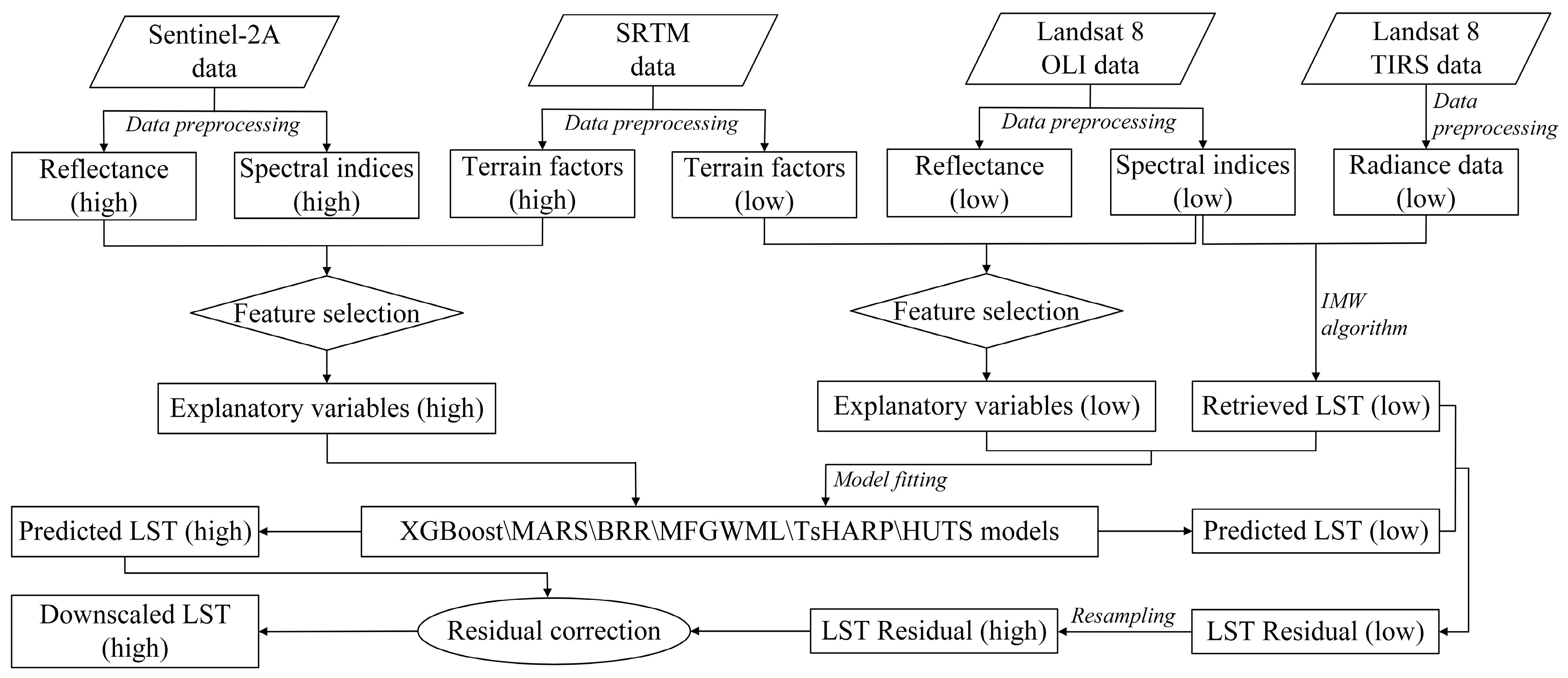
Figure 2 displays the overall technique flowchart of the LST downscaling procedures in this study. The LST downscaling from 30 to 10 m and the six downscaling schemes designed for validation were carried out according to the following workflow.
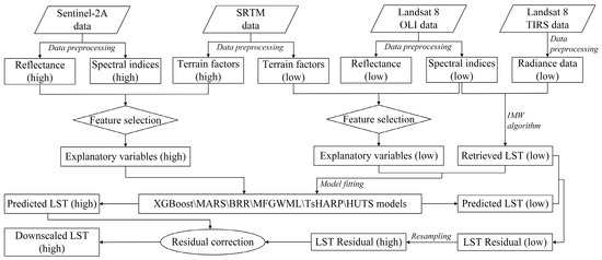
Figure 2.
Flowchart of the LST downscaling procedure. IMW, improved mono-window; “(low)” and “(high)” represent coarse spatial resolution and relatively high spatial resolution, respectively.
3. Results
3.1. Feature Selection Procedure
3.1.1. Correlations between Features and LST
Table 5 summarizes the Pearson correlation coefficient values (abbreviated as P) between features and LST. Most features are moderately correlated () or highly correlated () with LST. Albedo, NIR, and SWIR1 are weakly correlated with LST (). Although they might be useless individually, they can significantly improve the model performance when employed with other features [37]. However, aspect and hillshade were removed, as they are almost irrelevant to LST ().

Table 5.
Pearson correlation coefficients between features and LST.
3.1.2. Correlations among Features
The Pearson correlation coefficients (P) among features are listed in Table A1 of Appendix A. Among vegetation indices, FVC, index-based vegetation index (IVI), modified soil adjusted vegetation index (MSAVI), NDVI, optimal soil adjusted vegetation index (OSAVI), SAVI, and TC2 have extremely high correlations (). FVC was retained, and other vegetation indices were eliminated, given that FVC is the most relevant to LST among these features. Subsequently, other features with Pearson correlation coefficients less than 0.85 were selected based on the coefficient matrix. There were seven features selected in this stage: DEM, FVC, MNDWI, NIR, slope, SWIR2, and TC1.
3.1.3. Variable Importance Assessment
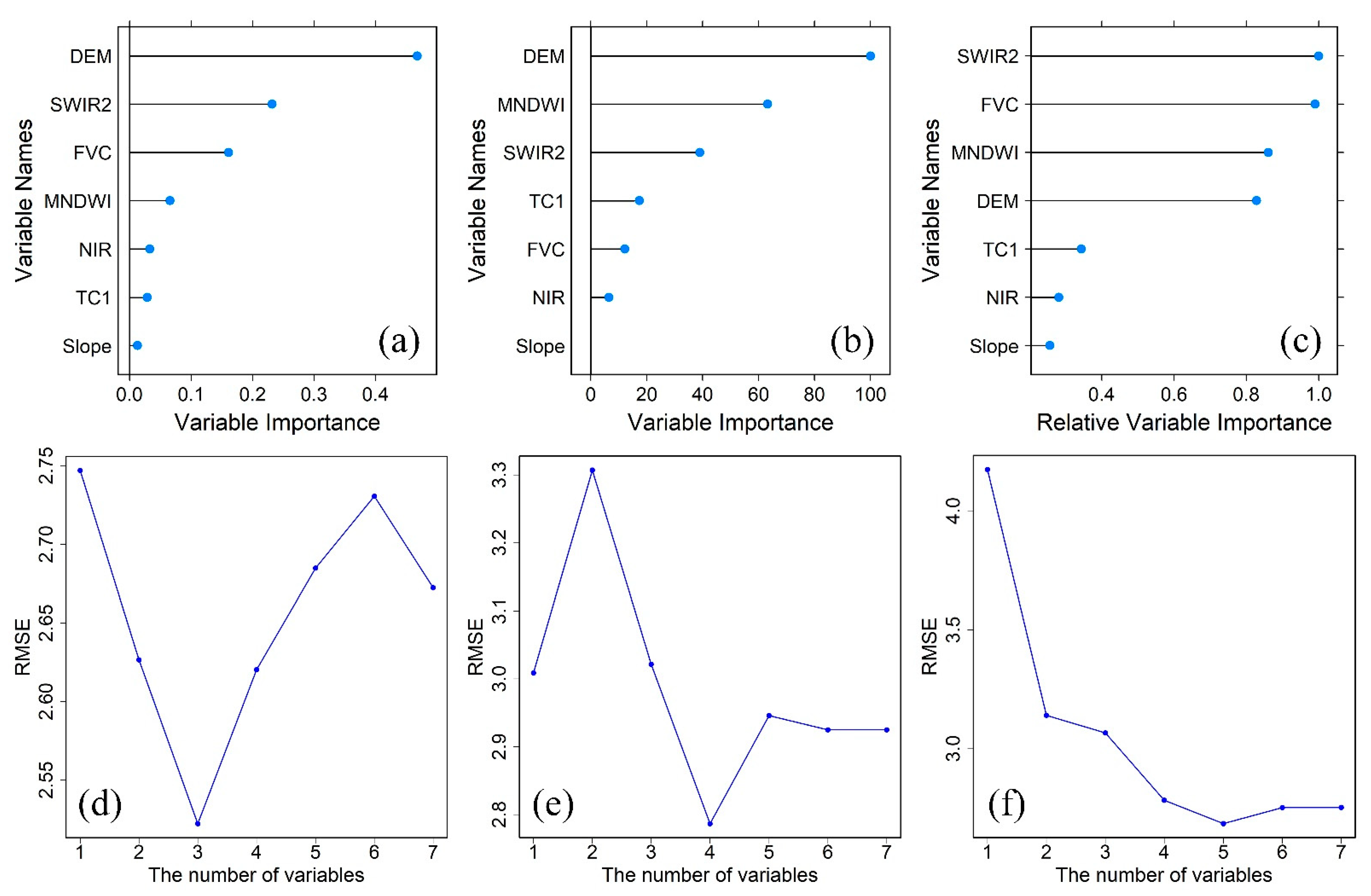
To identify the optimal feature combination for each model, we separately added the previously selected features to the three base models according to the variable importance rankings provided by each model, in descending order (Figure 3a–c). The RMSE values of the models with different numbers of variables were calculated (Figure 3c–e). The lowest RMSE value of each model indicates the optimal variable number. Therefore, the optimal feature combination for the XGBoost model is the combination of the top three variables, namely DEM, SWIR2, and FVC. The optimal feature combination for the MARS model is the combination of the top four variables, namely DEM, MNDWI, SWIR2, and TC1. The optimal feature combination for the BRR model is the combination of the top five variables, namely SWIR2, FVC, MNDWI, DEM, and TC1.
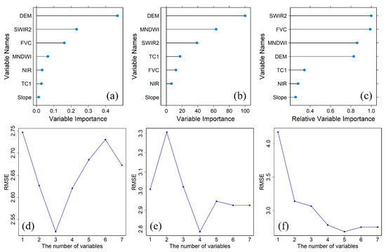
Figure 3.
Graphs (a–c) display the scores and ranks of the variable importance provided by the XGBoost, multivariate adaptive regression splines (MARS), and Bayesian ridge regression (BRR) models, respectively. Graphs (d–f) display the predictive root mean square error (RMSE) values (K) of the XGBoost, MARS, and BRR models, respectively, varying with the number of variables.
3.2. MFGWML Model Analysis
3.2.1. Base Model Correlations
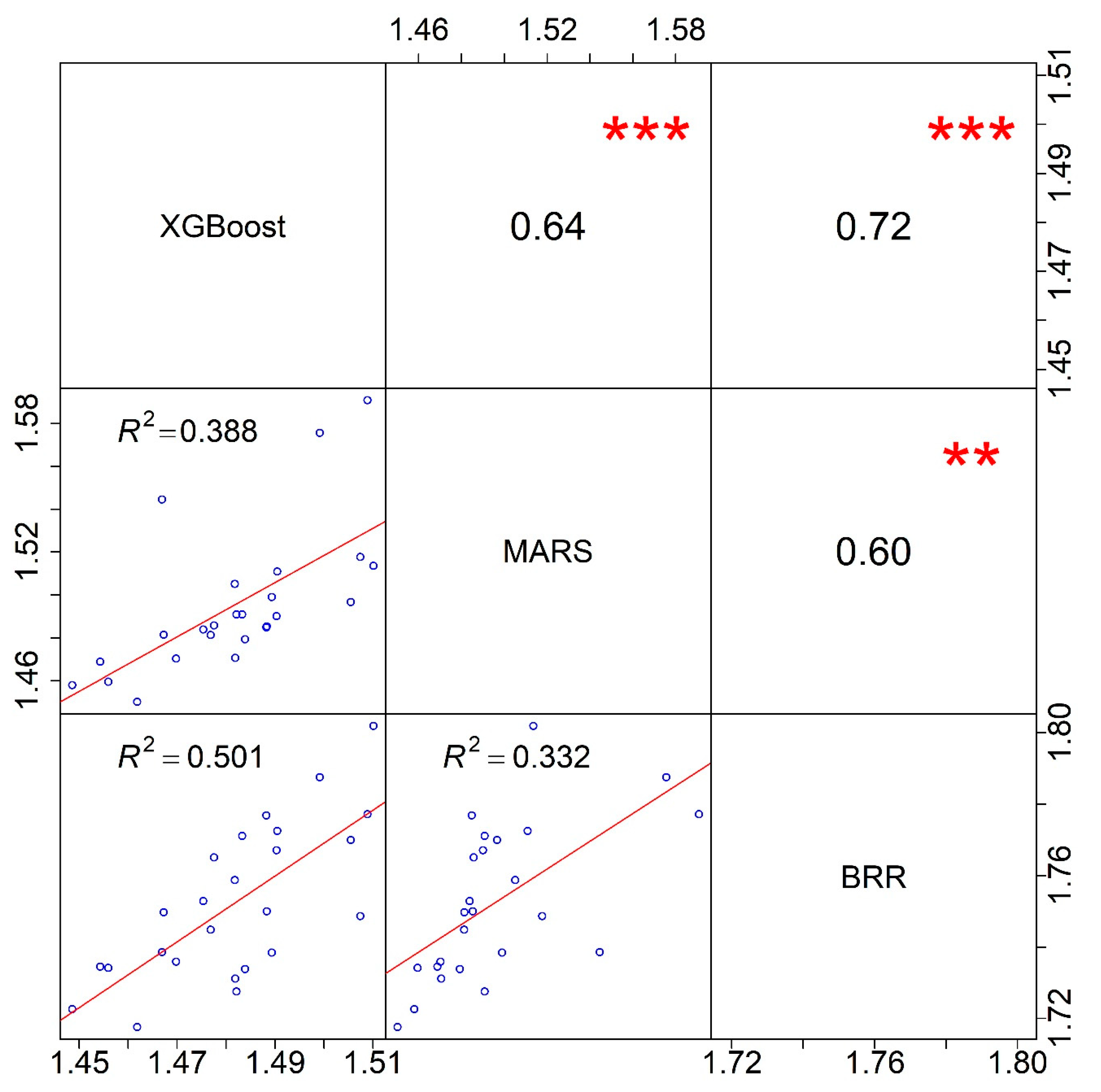
Figure 4 displays the correlation coefficients among the XGBoost, MARS, and BRR models. All the correlation coefficient values are less than 0.75, which indicates that the three base models have weak relationships; thus, they can be fused to improve predictions.
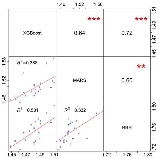
Figure 4.
The scatterplot matrix illustrates the correlations among the XGBoost, MARS, and BRR models. Model names are shown along the diagonal. The bivariate scatterplots (hollow blue circles) with a fitted red line are shown below the diagonal. The correlation values are shown above the diagonal. Two asterisks and three asterisks represent significance levels with p-values of 0.001 and 0, respectively.
3.2.2. MFGWML Model Parameters
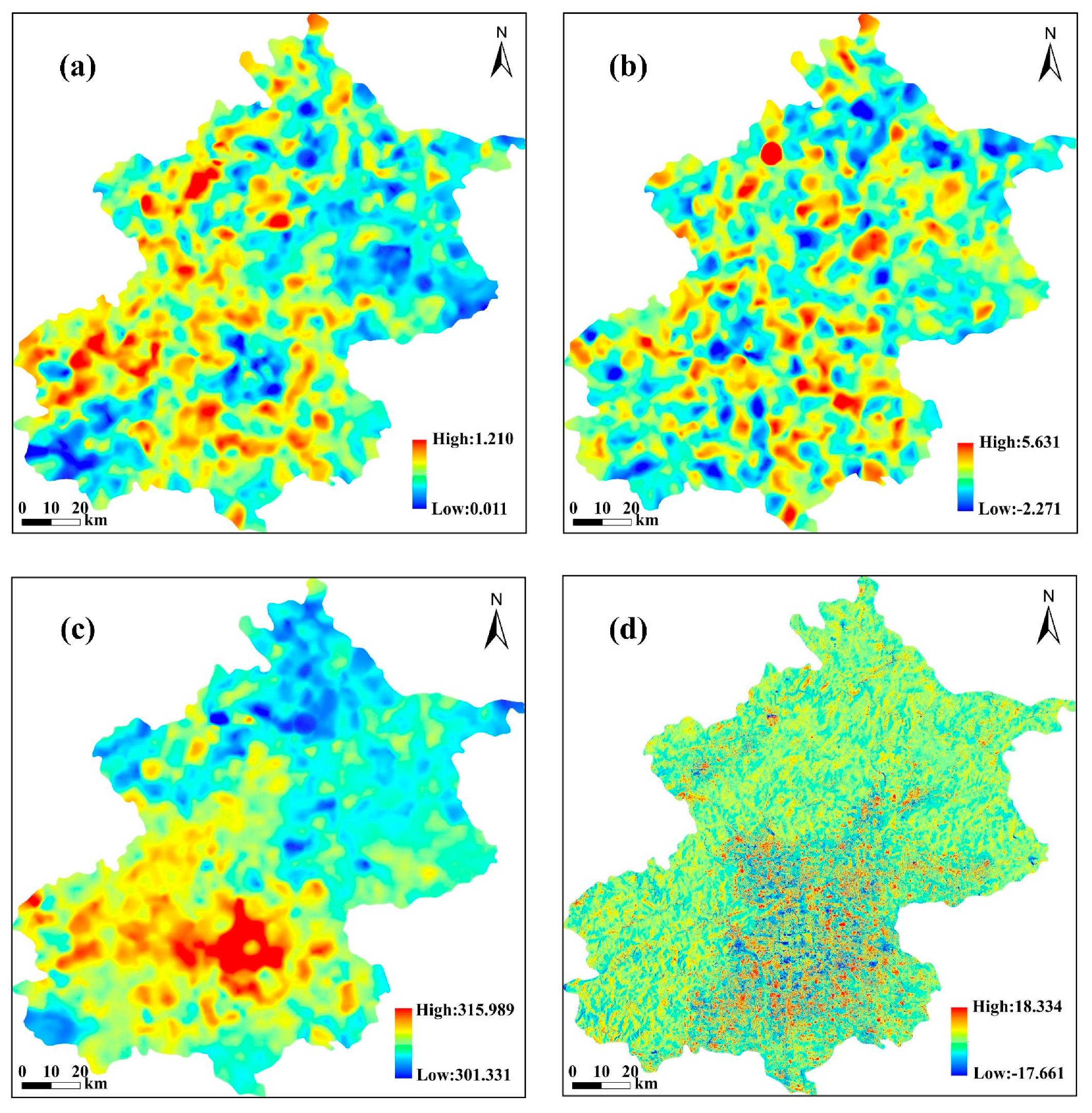
As shown in Figure 5, the regression coefficients (namely the slope of PC1 and the slope of PC2), intercept, and residual for the MFGWML model with a spatial resolution of 30 m represent evident spatial heterogeneity. Therefore, it is essential to utilize the local model, namely GWR, to characterize the spatially nonstationary relationships between LST and explanatory variables (PC1 and PC2). Moreover, these parameters were resampled from 30 to 10 m with the nearest neighbor resampling method for predicting the 10 m LST.
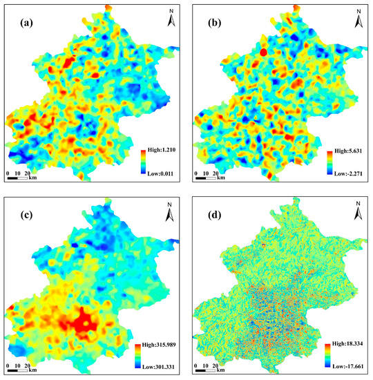
Figure 5.
Spatial distribution of the 30 m multi-factor geographically weighted machine learning (MFGWML) model parameters: (a) slope of principal component 1 (PC1), (b) slope of PC2, (c) intercept (K), and (d) residual.
3.3. Accuracy Validation and Comparison
3.3.1. Comparing MFGWML with TsHARP
The downscaling results of MFGWML and TsHARP are compared after excluding water regions. Water regions were identified, using the water mask built by setting the threshold “” to the MNDWI image. As shown in Figure 6, the MFGWML downscaled result has a more similar spatial pattern distribution to that of the original 30 m LST data than the TsHARP downscaled result. There are many overestimations in the TsHARP downscaled result. These results illustrate that MFGWML can recognize and retain LST heterogeneity much better than TsHARP.
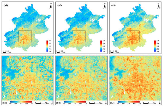
Figure 6.
Spatial distribution of the water-masked LST (K) data. (a1) Retrieved 30 m LST (K) data, (a2) MFGWML downscaled 10 m LST (K) data, and (a3) thermal image sharpening (TsHARP) downscaled 10 m LST (K) data. Plots (b1–b3) are the corresponding subsets of plots (a1–a3), respectively. The black rectangle is the minimum bounding rectangle of the central urban area; it represents the spatial extent of the subset. The blanks in these plots denote no-data areas due to the exclusion of water regions.
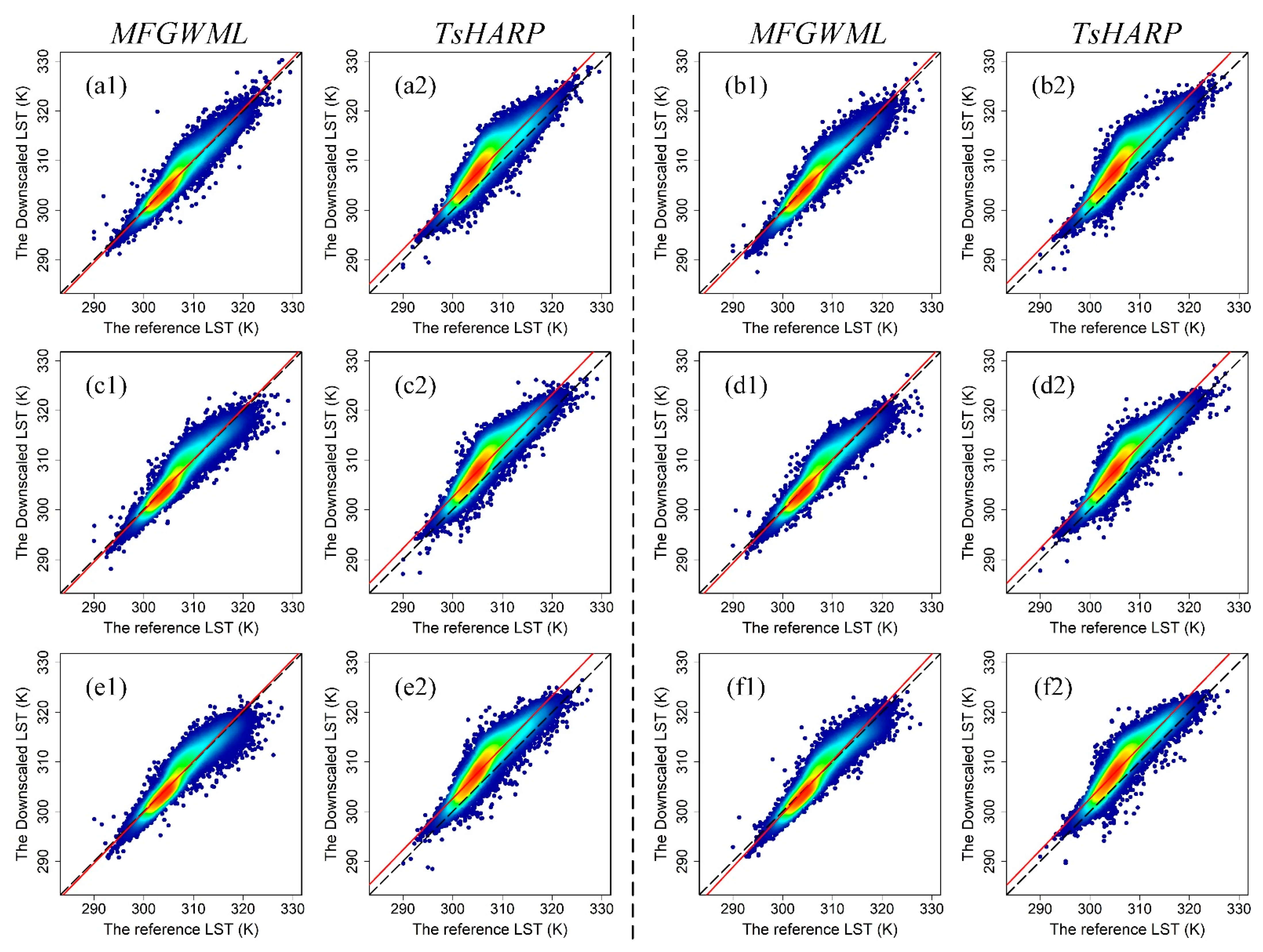
A total of 50,000 points were randomly selected from the entire city of Beijing (excluding water regions), to assess the model performances of MFGWML and TsHARP. The pixel-based scatterplots of the downscaled LST data produced by MFGWML and TsHARP against the corresponding reference LST data for the six downscaling schemes are presented in Figure 7. The fitting line of scatters in the MFGWML model is closer to the reference line than that of scatters in the TsHARP model for each downscaling scheme. Table 6 lists the statistical parameters of the fitting lines. The slope values for the fitting line of MFGWML and TsHARP are very close. However, the RMSE and MAE values for the fitting equation of MFGWML are lower than those of TsHARP for each downscaling scheme. The value for the fitting equation of MFGWML is higher than that of TsHARP for each downscaling scheme. Most scatter points in the MFGWML model are generally distributed on the reference line, which represents a 1:1 relationship. However, most scatter points in the TsHARP model tend to be located above the reference line, which indicates that TsHARP overestimates the downscaled LST data for the six downscaling schemes. The results confirm that the single explanatory variable, namely the NDVI, in the TsHARP model is incapable of capturing the complicated spatial heterogeneity characteristics of LST data. MFGWML outperforms TsHARP and is robust at different scales.
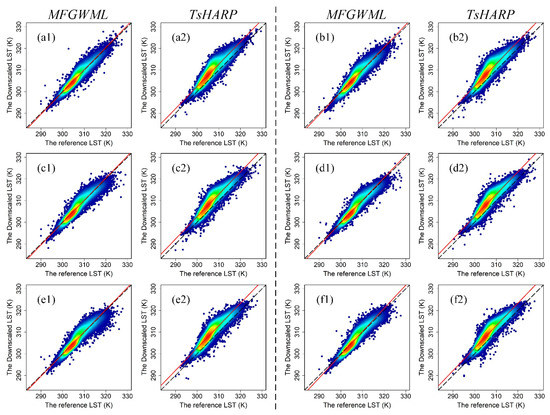
Figure 7.
Pixel-based density scatterplots of the downscaled LST (K) data (Y-axis) and reference LST (K) data (X-axis) for the six downscaling schemes: (a1,a2,b1,b2,c1,c2,d1,d2,e1,e2,f1,f2). Plots (a1,a2) are the density scatterplots for Scheme 1, which corresponds to the MFGWML model and TsHARP model, respectively. The remainder of the plots are named in the same manner. The dotted black line is the 1:1 reference line, and the solid red line is the fitting line.

Table 6.
Statistical parameters of the fitting lines for scatters in MFGWML and TsHARP for the six downscaling schemes performed in the entire Beijing (excluding water regions).
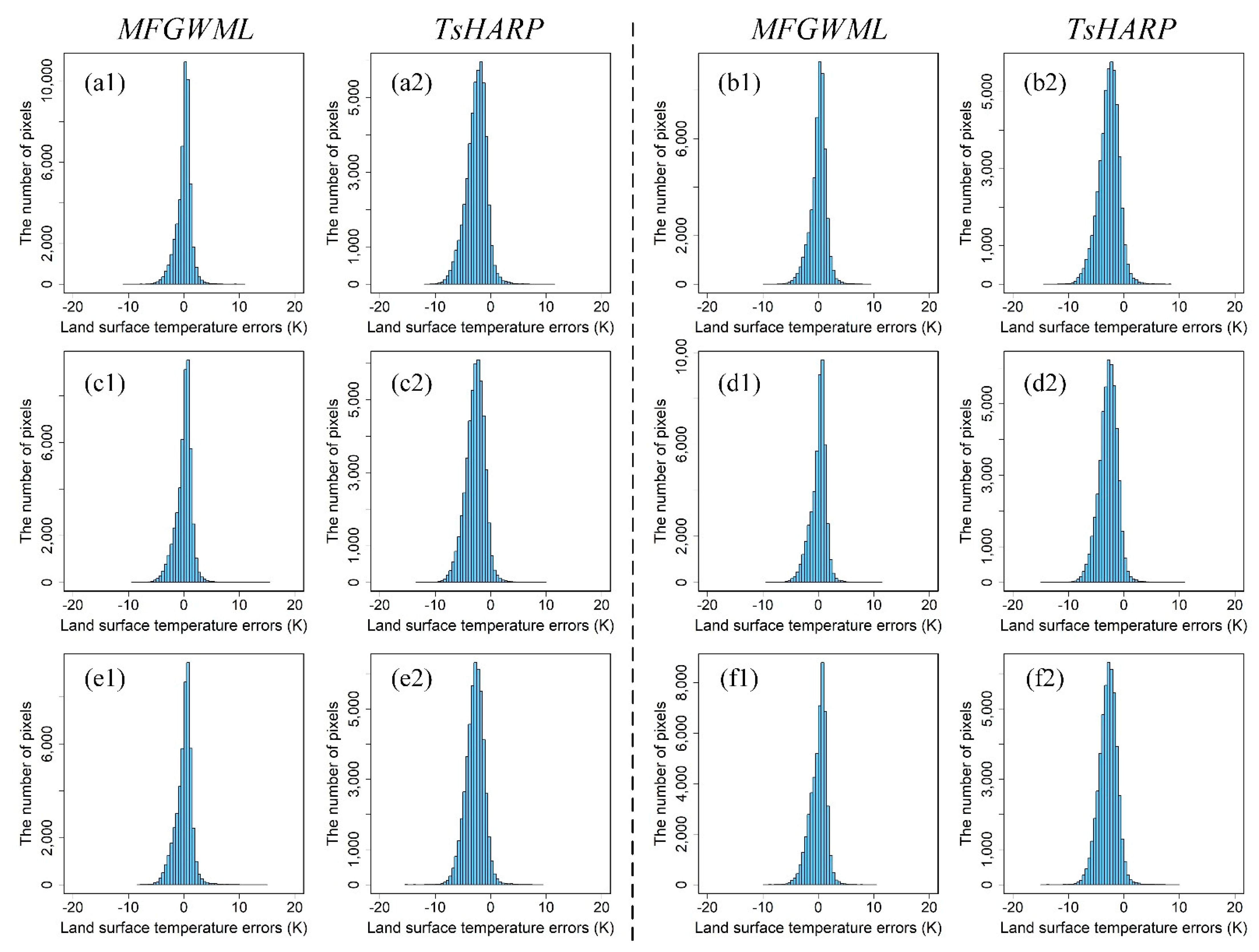
Figure 8 shows the LST error distribution histograms of the MFGWML and TsHARP models for the six downscaling schemes. Intuitively, the LST errors of the MFGWML model for the six downscaling schemes are concentrated near 0 K. However, the LST errors of the TsHARP model for the six downscaling schemes tend to be less than 0 K, which indicates that TsHARP performs worse than MFGWML at different scales.
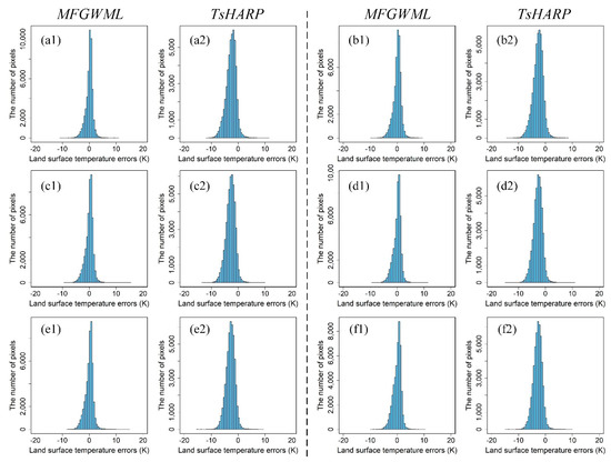
Figure 8.
LST error distribution histograms of the MFGWML and TsHARP models for the six downscaling schemes: (a1,a2,b1,b2,c1,c2,d1,d2,e1,e2,f1,f2). Plots (a1,a2) represent the LST error distribution histograms for Scheme 1, which corresponds to the MFGWML and TsHARP models, respectively. The remainder of the plots are named in the same manner.
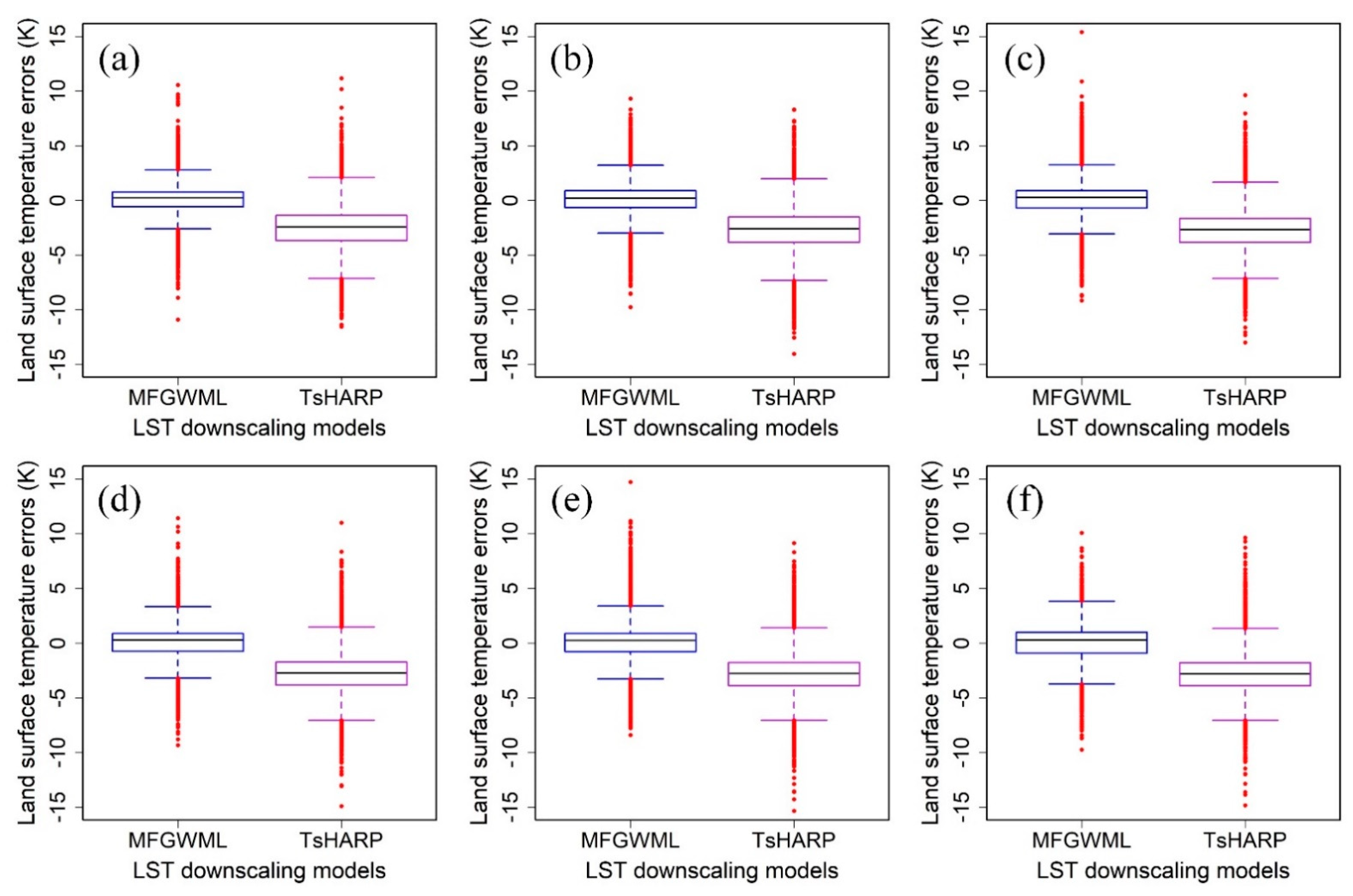
Figure 9 shows the LST error distribution boxplots of the MFGWML and TsHARP models for the six downscaling schemes. It is intuitively displayed that the median of LST errors in MFGWML for each scheme is almost 0 K, indicating that MFGWML is unbiased. The median of LST errors in TsHARP for each scheme is greater than -5 K and less than 0 K, indicating that TsHARP is biased. The interquartile range (IQR) is compared, which means the difference between the upper and lower quartiles of boxplots. The IQR for LST errors of MFGWML for each scheme is obviously narrower than that of TsHARP, indicating that the LST error distribution of MFGWML is more concentrated than that of TsHARP. Table 7 lists the exact values of the statistical indicators for evaluating LST error distributions. The means, medians, the 25th percentiles (marked as Q1), and the 75th percentiles (marked as Q3) for LST errors of MFGWML are closer to 0 K than those of TsHARP for the six downscaling schemes. Besides, the IQR values of MFGWML are less than those of TsHARP for the six downscaling schemes. These statistical results indicate that LST errors of MFGWML are more concentrated to 0 K than those of TsHARP. In other words, MFGWML performs better than TsHARP at different scales.
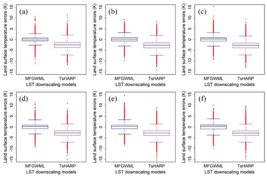
Figure 9.
LST error distribution boxplots of the MFGWML and TsHARP models for the six downscaling schemes: (a) Scheme 1, (b) Scheme 2, (c) Scheme 3, (d) Scheme 4, (e) Scheme 5, and (f) Scheme 6. The black line indicates the median value. The blue and purple boxes indicate the percentiles for the MFGWML and TsHARP models, respectively. The solid red dots indicate outliers.

Table 7.
Statistical indicators of LST error distribution in MFGWML and TsHARP for the six downscaling schemes performed in the entire city of Beijing (excluding water regions).
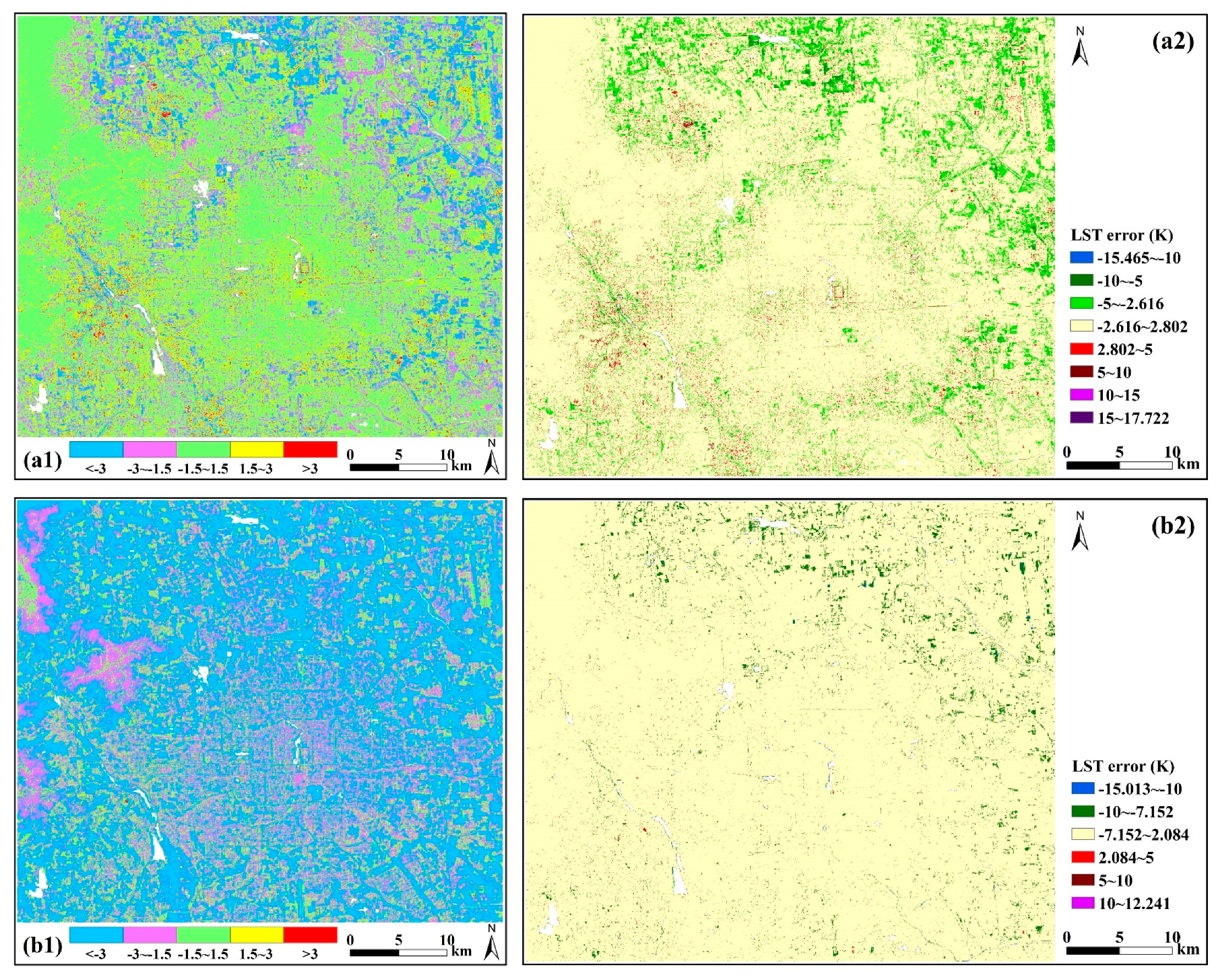
According to the above boxplots, there are outliers of LST errors in the MFGWML and TsHARP models for the six downscaling schemes. Pixels with LST error less than (Q1 − 1.5*IQR) or greater than (Q3 + 1.5*IQR) are identified as outliers. Figure 10 displays the spatial distribution of LST errors and their outliers in the MFGWML and TsHARP models for Scheme 1, namely downscaling from 90 to 30 m. Most LST errors in the MFGWML model range from −1.5 to 1.5 K (Figure 10a1), while most LST errors in the TsHARP model are less than −3 K (Figure 10a2). Table 8 shows that pixels with LST errors of <−3 K, −3 K to −1.5 K, −1.5 K to 1.5 K, 1.5 K to 3 K, and >3 K, account for 2.929%, 9.344%, 80.735%, 6.118%, and 0.874% of all the samples in the MFGWML model for Scheme 1, respectively. Pixels with LST errors of < −3 K, −3 K to −1.5 K, −1.5 K to 1.5 K, 1.5 K to 3 K, and >3 K, account for 37.389%, 34.695%, 26.939%, 0.703%, and 0.274% of all the samples in the TsHARP model for Scheme 1, respectively. Most outliers in the MFGWML model for Scheme 1 occurred in the northern and eastern parts of the urban area, ranging from −5 to −2.616 K. Most outliers in the TsHARP model for Scheme 1 also occurred in the northern and eastern parts of the urban area, but they range from −10 to −7.152 K. The outliers in the MFGWML model and TsHARP model for Scheme 1 account for 5.433% and 1.991%, respectively. The other five downscaling schemes have similar statistical results. These results indicate that the downscaled LSTs have few outliers, and the MFGWML downscaled LST is more reliable than the TsHARP downscaled LST.
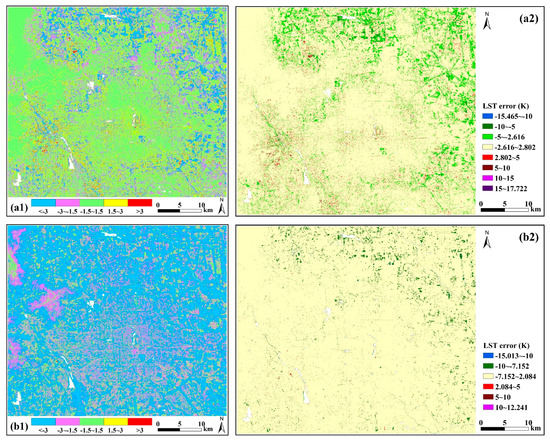
Figure 10.
Spatial distribution of LST errors (K) in the MFGWML and TsHARP models for Scheme 1. Plots (a1,b1) represent the spatial distribution of LST errors for MFGWML and TsHARP, respectively. Plots (a2,b2) indicate LST error outliers for MFGWML and TsHARP, respectively. In the plots (a2,b2), different colors except the light yellow color indicate outliers with different error ranges.

Table 8.
Proportional values of LST errors in MFGWML and TsHARP for the six downscaling schemes performed in the entire city of Beijing (excluding water regions).
Table 9 lists the accuracy evaluation indicators of MFGWML and TsHARP for the six downscaling schemes. In terms of Scheme 1, namely downscaling from 90 to 30 m, the Pearson coefficients for MFGWML and TsHARP are 0.964 and 0.932, respectively, which indicates that the downscaled LSTs generated by MFGWML and TsHARP are highly correlated with the reference LST. The RMSE values for TsHARP and MFGWML are 3.196 and 1.312 K, respectively. The MAE values for TsHARP and MFGWML are 2.707 and 0.961 K, respectively. These values demonstrate that MFGWML improves the results with a 58.949% decrease and a 64.499% decrease in the RMSE value and MAE value, respectively. The MBE values for TsHARP and MFGWML are and 0.006 K, respectively, indicating that MFGWML is more reliable than TsHARP. The NSE values for TsHARP and MFGWML are 0.510 and 0.917, respectively. The values for TsHARP and MFGWML are 0.631 and 0.917, respectively. These statistical results show that MFGWML outperforms TsHARP. The other five downscaling schemes have similar results, which indicates that MFGWML is robust at different scales.

Table 9.
Accuracy evaluation indicators of MFGWML and TsHARP for the six downscaling schemes performed in the entire city of Beijing (excluding water regions).
3.3.2. Comparing MFGWML with HUTS
As mentioned in Section 2.6.2, the HUTS algorithm was specifically proposed for LST downscaling in urban areas, where the spatial heterogeneity of land covers and LST is relatively considerable. Therefore, we performed the HUTS model for LST downscaling around the central urban area in Beijing. As shown in Figure 11, the MFGWML downscaled result has a more similar spatial pattern distribution to that of the original 30 m LST data than the HUTS downscaled result. There are many overestimations in the HUTS downscaled result. These results illustrate that MFGWML can recognize and retain LST heterogeneity much better than HUTS.

Figure 11.
Spatial distribution of LST (K) data around the central urban area. (a1) Retrieved 30 m LST (K) data, (a2) MFGWML downscaled 10 m LST (K) data, and (a3) the high-resolution urban thermal sharpener (HUTS) downscaled 10 m LST (K) data.
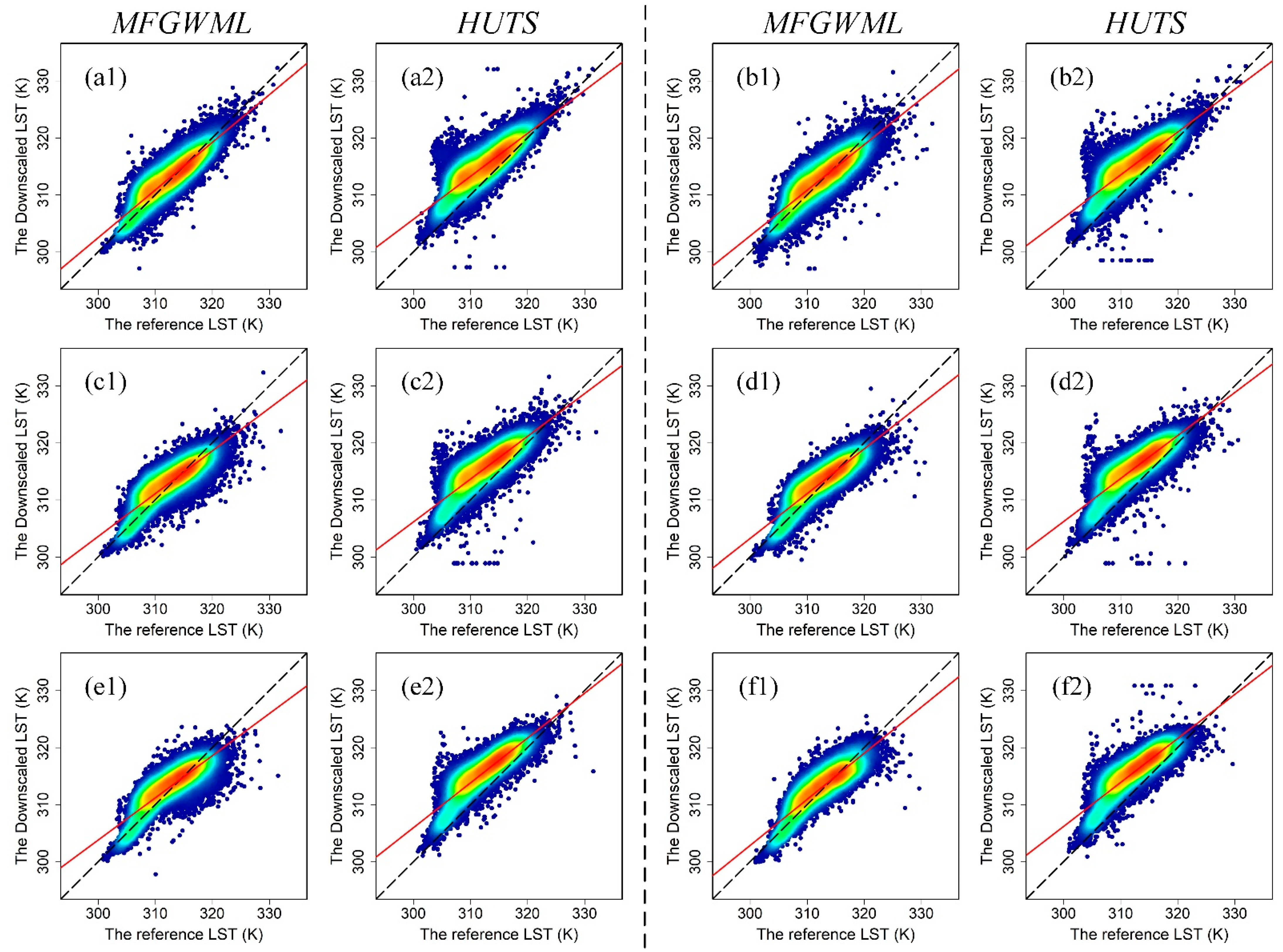
A total of 50,000 points were randomly selected around the central urban area to assess the model performances of MFGWML and HUTS. The pixel-based scatterplots of the downscaled LST data produced by MFGWML and HUTS against the corresponding reference LST data for the six downscaling schemes are presented in Figure 12. The fitting line of scatters in the MFGWML model is a little closer to the reference line than that of scatters in the HUTS model for each downscaling scheme. Table 10 lists the statistical parameters of the fitting lines. The slope values, RMSE values, MAE values, and values for the fitting lines of MFGWML and HUTS are very close in each downscaling scheme. Most scatter points in the MFGWML model generally distribute on the reference line, which represents a 1:1 relationship. However, most scatter points in the HUTS model tend to be located above the reference line, thus indicating that the HUTS model overestimates the downscaled LST data for the six downscaling schemes. The results demonstrate that the two factors (namely NDVI and albedo) in the HUTS model are incapable of capturing the LST heterogeneity. MFGWML outperforms HUTS and is robust at different scales.
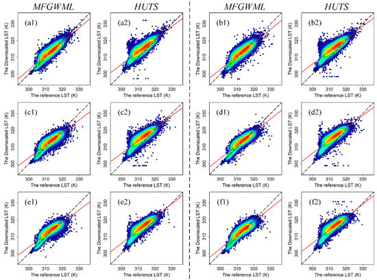
Figure 12.
Density scatterplots of per-pixel comparison between the downscaled LST (K) data (Y-axis) and the reference LST (K) data (X-axis) at different scales (a1,a2,b1,b2,c1,c2,d1,d2,e1,e2,f1,f2). Plots (a1,a2) are the density scatterplots for Scheme 1, which corresponds to the MFGWML and HUTS models, respectively. The remainder of the plots are named in the same manner. The dotted black line is the 1:1 reference line, and the solid red line is the fitting line.

Table 10.
Statistical parameters for the fitting lines of scatters in MFGWML and HUTS for the six downscaling schemes performed around the central urban area.
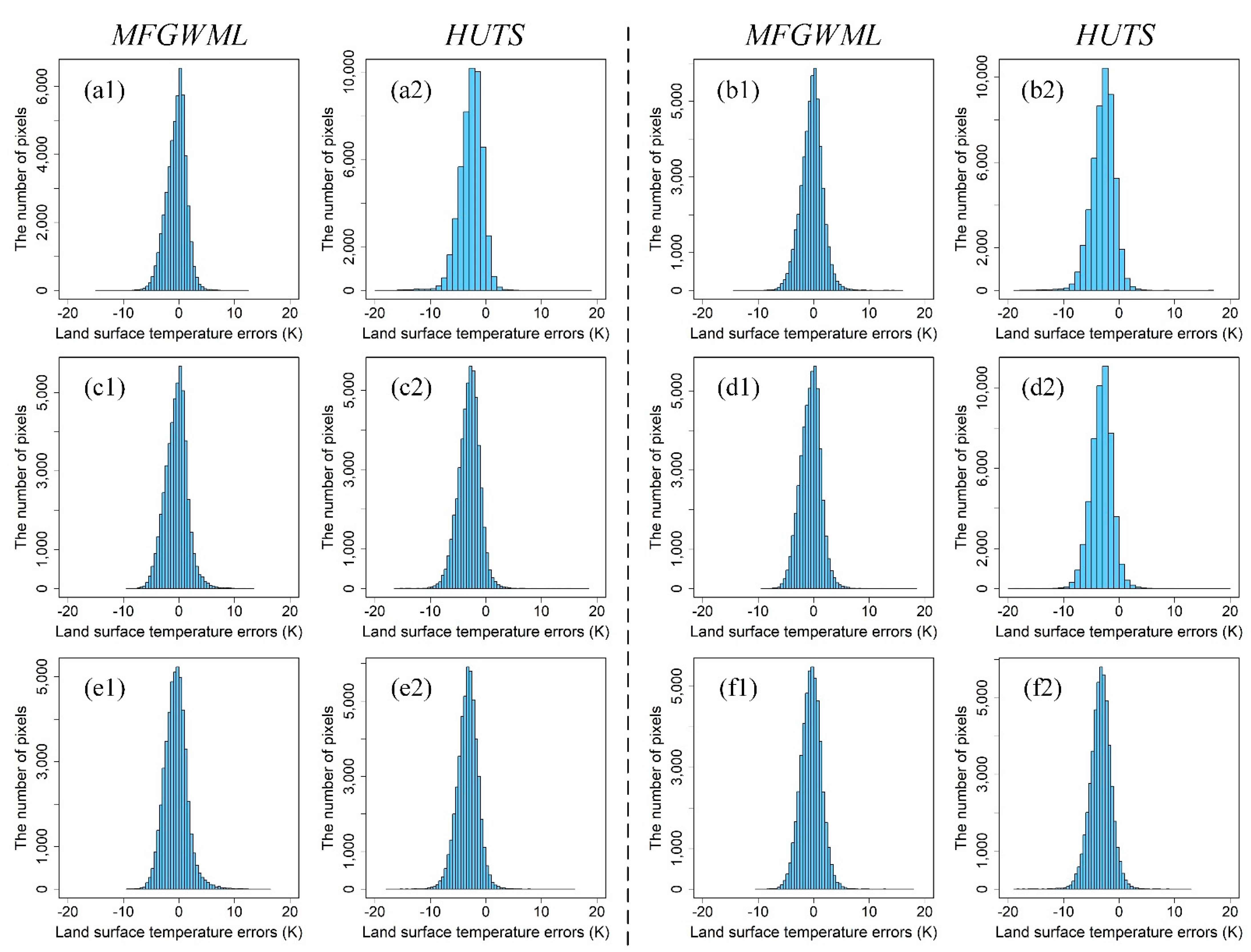
Figure 13 displays the LST error distribution histograms of the MFGWML and HUTS models for the six downscaling schemes. Intuitively, the LST errors of the MFGWML model for the six downscaling schemes are concentrated near 0 K. However, the LST errors of the HUTS model for the six downscaling schemes tend to be less than 0 K, which indicates that HUTS performs worse than MFGWML at different scales.
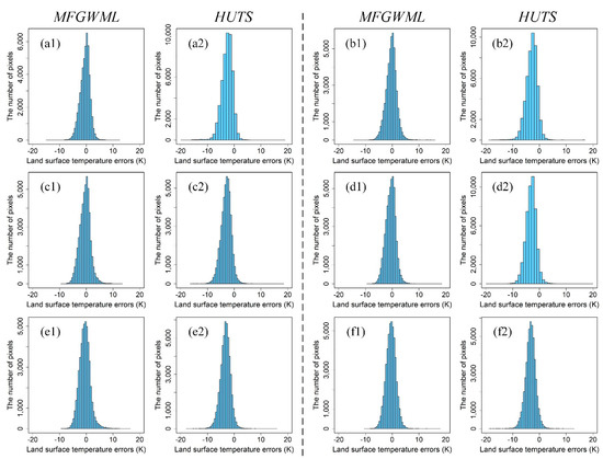
Figure 13.
LST error distribution histograms of the MFGWML and HUTS models for the six downscaling schemes: (a1,a2,b1,b2,c1,c2,d1,d2,e1,e2,f1,f2). Plots (a1,a2) represent the LST error distribution histograms for Scheme 1, which corresponds to the MFGWML and HUTS models, respectively. The remainder of the plots are named in the same manner.
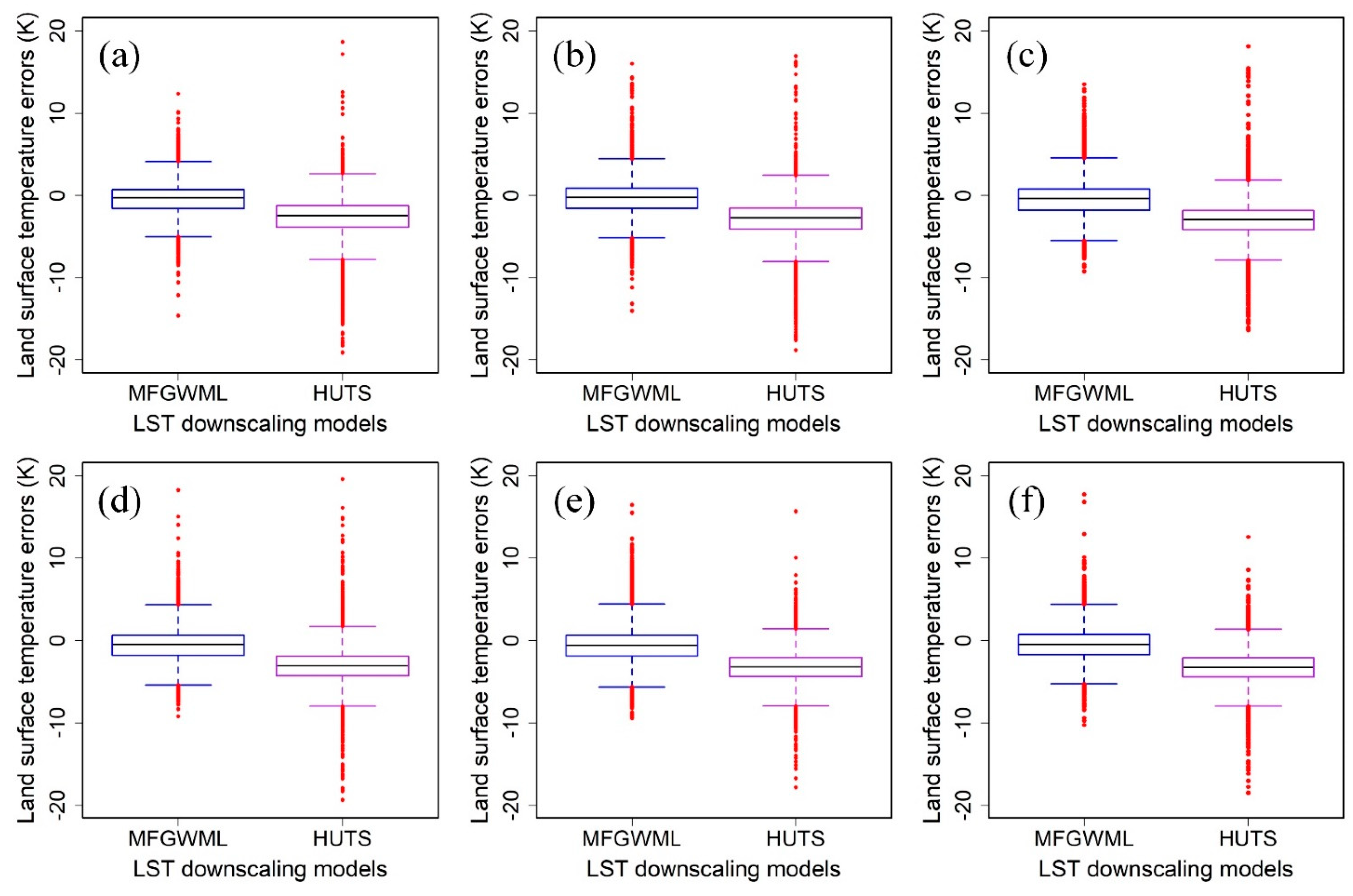
Figure 14 shows the LST error distribution boxplots of the MFGWML and HUTS models for the six downscaling schemes. It is intuitively displayed that the median of LST errors in MFGWML for each scheme is almost 0 K, indicating that MFGWML is unbiased. The median of LST errors in HUTS for each scheme is greater than and less than 0 K, indicating that HUTS is biased. The IQRs of LST errors in MFGWML and HUTS are almost the same, indicating that the LST errors in MFGWML and HUTS have the same dispersion. Table 11 lists the exact values of the statistical indicators for evaluating LST errors. It is evident that the means, medians, the 25th percentiles, and the 75th percentiles for LST errors of MFGWML are closer to 0 K than those of HUTS for the six downscaling schemes. The IQR values of MFGWML are a little less than those of HUTS for Scheme 1 and Scheme 2, while the IQR values of MFGWML are a little greater than those of HUTS for Scheme 3, Scheme 4, Scheme 5, and Scheme 6. In general, The IQR values of MFGWML and HUTS are very close for the six downscaling schemes, indicating that the degrees of LST error dispersion in MFGWML and HUTS are almost the same. The above statistical results indicate that LST errors in MFGWML are concentrated to 0 K while those in HUTS are concentrated to a value less than 0 K. In other words, MFGWML performs better than HUTS at different scales.
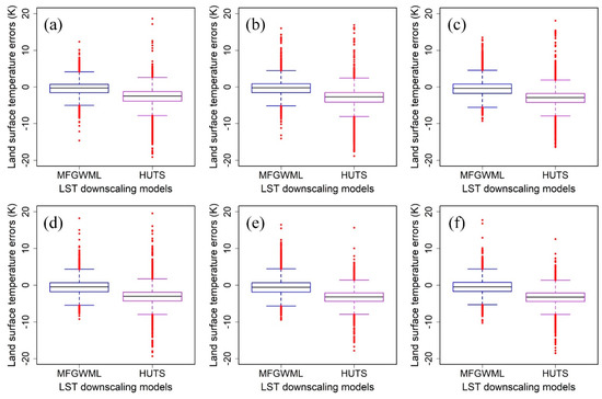
Figure 14.
LST error distribution boxplots of the MFGWML and HUTS models for the six downscaling schemes: (a) Scheme 1, (b) Scheme 2, (c) Scheme 3, (d) Scheme 4, (e) Scheme 5, and (f) Scheme 6. The black line indicates the median value. The blue and purple boxes indicate the percentiles for the MFGWML and HUTS models, respectively. The solid red dots indicate outliers.

Table 11.
Statistical indicators of LST error distribution in MFGWML and HUTS for six downscaling schemes performed around the central urban area.
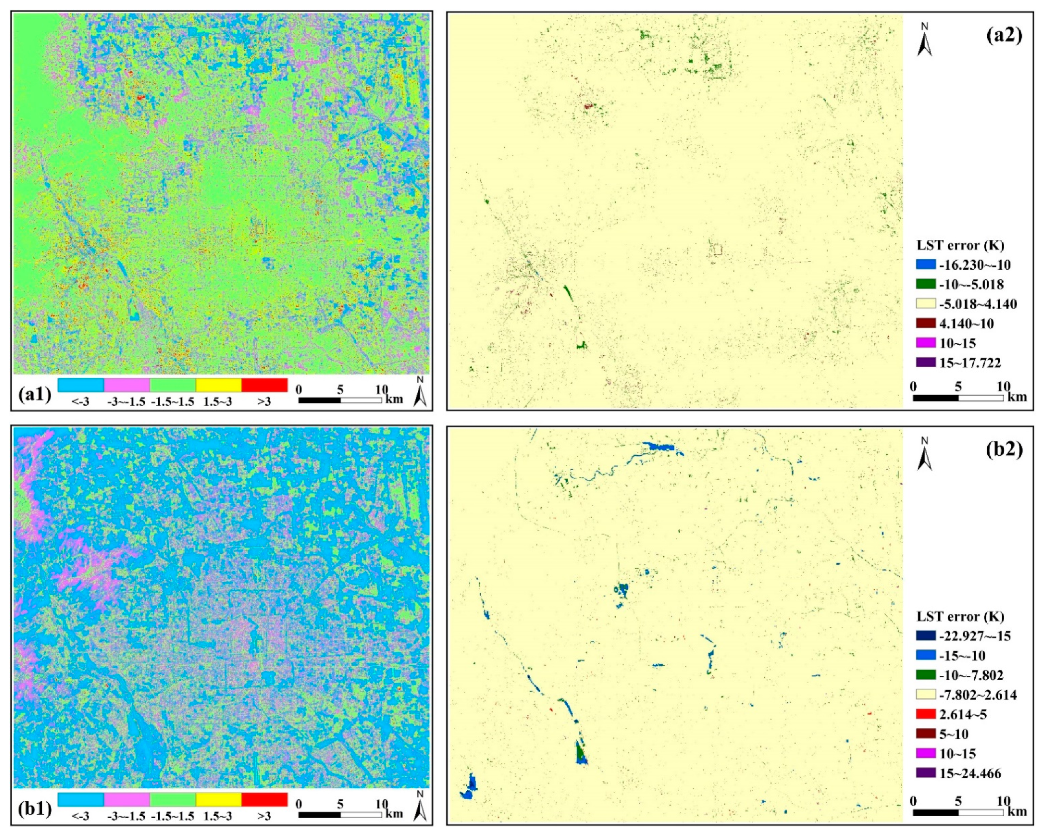
Figure 15 displays the spatial distribution of LST errors and their outliers in the MFGWML and HUTS models for Scheme 1, namely downscaling from 90 to 30 m. Most LST errors in the MFGWML model range from −1.5 to 1.5 K (Figure 15a1), while most LST errors in the HUTS model are less than −3 K (Figure 15a2). Table 12 shows that the pixels with LST errors of <−3 K, −3 K to −1.5 K, −1.5 K to 1.5 K, 1.5 K to 3 K, and >3 K, account for 8.790%, 17.512%, 62.838%, 9.259%, and 1.601% of all the samples in the MFGWML model for Scheme 1, respectively. Pixels with LST errors of < −3 K, −3 K to −1.5 K, −1.5 K to 1.5 K, 1.5 K to 3 K, and > 3 K, account for 39.714%, 30.830%, 28.643%, 0.673%, and 0.140% of all the samples in the HUTS model for Scheme 1, respectively. Most outliers in the MFGWML model for Scheme 1 occurred in the northern part of the urban area, ranging from −10 to −5.018 K. Most outliers in the HUTS model for Scheme 1 occurred in the northern and southwestern parts of the urban area, ranging from −15 to −10 K. The outliers in the MFGWML and HUTS models for Scheme 1 are few, accounting for 1.359% and 1.332%, respectively. The other five downscaling schemes have similar statistical results. These results indicate that the MFGWML downscaled LST is more reliable than the HUTS downscaled LST.

Figure 15.
Spatial distribution of LST errors (K) in the MFGWML and HUTS models for Scheme 1. Plots (a1,b1) represent the spatial distribution of LST errors in the MFGWML and HUTS models, respectively. Plots (a2,b2) indicate LST error outliers for MFGWML and HUTS, respectively. In the plots (a2,b2), different colors, except for the light yellow color, indicate outliers with different ranges of LST errors.

Table 12.
Proportional values of LST errors in MFGWML and HUTS for the six downscaling schemes performed around the central urban area.
Table 13 lists the accuracy evaluation indicators of MFGWML and HUTS for the six downscaling schemes. In terms of Scheme 1, namely downscaling from 90 to 30 m, the Pearson coefficients for MFGWML and HUTS are 0.904 and 0.869, respectively, which indicates that the downscaled LSTs generated by MFGWML and HUTS are highly correlated with the reference LST. The RMSE values for HUTS and MFGWML are 3.366 and 1.834 K, respectively. The MAE values for HUTS and MFGWML are 2.779 K and 1.407 K, respectively. These values demonstrate that MFGWML improves the results with a 45.514% decrease and a 49.370% decrease in the RMSE value and MAE value, respectively. The MBE values for HUTS and MFGWML are and , respectively, indicating that MFGWML is more reliable than HUTS. The NSE values for HUTS and MFGWML are 0.342 and 0.805, respectively. The values for HUTS and MFGWML are 0.534 and 0.807, respectively. These statistical results show that MFGWML outperforms HUTS. The other five downscaling schemes have similar results, which indicates that the MFGWML model is robust at different scales.

Table 13.
Accuracy evaluation indicators of MFGWML and HUTS for the six downscaling schemes implemented around the central urban area.
4. Discussion
4.1. Sources of LST Errors
The sources of LST errors in this paper mainly include three aspects. First, LST errors may come from the spectral differences due to the different acquisition dates of Landsat 8 and Sentinel-2A images. Second, there are inevitable errors generated in the LST retrieval procedures and the aggregation processing of the original retrieved LST data and the explanatory variables. Third, residual calibration is an important means to eliminate the uncertainty of model outputs. However, the nearest neighbor resampling method performed on the coarse-resolution residual is incapable of eliminating the uncertainty of model outputs. Therefore, there are some LST errors generated in the residual calibration procedures.
4.2. Limitations
This study has two shortcomings. First, the selected Landsat 8 and Sentinel-2A images have different acquisition dates due to the lack of appropriate images. Nevertheless, given that their dates are very similar, the spectral differences within several days in summer are expected to be very small. Second, the input PCA components (PC1 and PC2) make the model interpretability of MFGWML relatively weak. However, the MFGWML model requires PCA due to the effects of local multicollinearity.
4.3. Future Research
Further studies involve the following three aspects. First, the multicollinearity issue in GWR needs further investigation to improve the interpretability of the MFGWML model. Recently, Fotheringham, one of the GWR algorithm developers, demonstrated that GWR is very robust to multicollinearity influences and appealed to reconsider the previous contention [69]. Second, more validation strategies for downscaled LST data need more explorations, due to the lack of corresponding ground measurements at the satellite transit time. Third, the applicability, sensitivity, and uncertainty of the MFGWML model should be investigated for LST downscaling in areas with different climatic, environmental, and economic characteristics.
5. Conclusions
This study proposed the MFGWML downscaling method, to generate reliable and robust high-resolution LST data based on Sentinel-2A images. The MFGWML model introduced GWR to obtain geographically weighted ensemble predictions based on three different types of excellent machine learners (namely XGBoost, MARS, and BRR). By comparing the performances of different LST downscaling models, the main conclusions are summarized as follows:
(1) The multi-factor downscaling model performs better than the classic single-factor algorithm, namely TsHARP. This conclusion is consistent with those of many previous studies. The multi-factor downscaling model outperforms the classic two-factor method, namely HUTS. This paper demonstrates that both the single indicator (namely NDVI) in TsHARP and the two factors (namely NDVI and albedo) in HUTS are insufficient for capturing the LST heterogeneity.
(2) The experimental results for the six LST downscaling schemes also indicate that MFGWML is robust at different scales.
(3) The MFGWML model integrates the advantages of multi-factor regressions, nonparametric ML algorithms, and the GWR method, to recognize the local heterogeneity and generate reliable and robust LST data.
MFGWML is a practical downscaling approach for obtaining LST data with relatively high spatial resolution, reliability, and robustness. The detailed spatial heterogeneity information of high-resolution LST data produced by MFGWML can promote LST applications in urban climate and other environmental research. The MFGWML method can also be applied for high-spatial-resolution predictions of other land surface variables and meteorological parameters (such as wind speed), which involve multiple influential factors.
Author Contributions
Conceptualization, S.X., Q.Z., G.H., Z.Z., and K.Y.; methodology, S.X., Q.Z., and K.Y.; software, S.X. and G.W.; validation, S.X. and M.W.; formal analysis, S.X., Q.Z., and K.Y.; investigation, S.X., N.Z., and M.W.; resources, Q.Z., G.H., Z.Z., K.Y., and N.Z.; data curation, S.X., G.W., and M.W.; writing—original draft, S.X.; writing—review and editing, S.X., Q.Z., G.H., Z.Z., K.Y., and G.W.; visualization, S.X., G.W., and M.W.; supervision, Q.Z., G.H., Z.Z., K.Y., and N.Z.; project administration, Q.Z., G.H., Z.Z., K.Y., N.Z., and G.W.; funding acquisition, Q.Z., G.H., Z.Z., K.Y., N.Z., and G.W. All authors have read and agreed to the published version of the manuscript.
Funding
This research was funded by the National Key R&D Program of China (No. 2017YFB0503902) and the National Natural Science Foundation of China (No. 61731022 and No. 61860206004).
Institutional Review Board Statement
Not applicable.
Informed Consent Statement
Not applicable.
Acknowledgments
We thank the editors and the anonymous reviewers for their insightful comments and valuable suggestions. Meanwhile, we thank associate professor Mengmeng Wang (China University of Geosciences) for his insightful suggestions.
Conflicts of Interest
The authors declare no conflict of interest.
Appendix A

Table A1.
Pearson correlation coefficient matrix among the candidate features.
Table A1.
Pearson correlation coefficient matrix among the candidate features.
| Features | Albedo | BI | Blue | DEM | FVC | Green | IBI | IVI | MNDWI | MSAVI | NDBI | NDDI | NDVI | NDWI | NIR | OSAVI | Red | SAVI | Slope | SWIR1 | SWIR2 | TC1 | TC2 | TC3 | UI |
|---|---|---|---|---|---|---|---|---|---|---|---|---|---|---|---|---|---|---|---|---|---|---|---|---|---|
| Albedo | 1.000 | 0.196 | 0.456 | −0.029 | −0.040 | 0.549 | 0.149 | 0.092 | −0.239 | 0.187 | 0.242 | 0.043 | −0.003 | −0.088 | 0.671 | 0.082 | 0.465 | 0.161 | −0.081 | 0.870 | 0.627 | 0.958 | 0.137 | −0.416 | 0.220 |
| BI | 0.196 | 1.000 | 0.797 | −0.499 | −0.913 | 0.813 | 0.968 | −0.843 | 0.532 | −0.854 | 0.978 | −0.815 | −0.862 | 0.771 | −0.529 | −0.868 | 0.875 | −0.851 | −0.463 | 0.543 | 0.824 | 0.460 | −0.852 | −0.796 | 0.972 |
| Blue | 0.456 | 0.797 | 1.000 | −0.505 | −0.828 | 0.960 | 0.776 | −0.788 | 0.575 | −0.750 | 0.805 | −0.787 | −0.814 | 0.749 | −0.335 | −0.800 | 0.950 | −0.767 | −0.491 | 0.575 | 0.858 | 0.642 | −0.795 | −0.623 | 0.864 |
| DEM | −0.029 | −0.499 | −0.505 | 1.000 | 0.611 | −0.486 | −0.435 | 0.534 | −0.513 | 0.555 | −0.454 | 0.529 | 0.534 | −0.520 | 0.381 | 0.540 | −0.482 | 0.533 | 0.679 | −0.139 | −0.375 | −0.161 | 0.536 | 0.276 | −0.507 |
| FVC | −0.040 | −0.913 | −0.828 | 0.611 | 1.000 | −0.808 | −0.845 | 0.963 | −0.807 | 0.951 | −0.858 | 0.953 | 0.974 | −0.932 | 0.674 | 0.973 | −0.858 | 0.955 | 0.595 | −0.302 | −0.693 | −0.294 | 0.937 | 0.580 | −0.922 |
| Green | 0.549 | 0.813 | 0.960 | −0.486 | −0.808 | 1.000 | 0.755 | −0.746 | 0.540 | −0.695 | 0.798 | −0.754 | −0.783 | 0.713 | −0.225 | −0.755 | 0.974 | −0.712 | −0.477 | 0.660 | 0.871 | 0.733 | −0.730 | −0.623 | 0.840 |
| IBI | 0.149 | 0.968 | 0.776 | −0.435 | −0.845 | 0.755 | 1.000 | −0.796 | 0.415 | −0.836 | 0.984 | −0.744 | −0.798 | 0.694 | −0.561 | −0.828 | 0.835 | −0.830 | −0.383 | 0.514 | 0.809 | 0.411 | −0.850 | −0.812 | 0.961 |
| IVI | 0.092 | −0.843 | −0.788 | 0.534 | 0.963 | −0.746 | −0.796 | 1.000 | −0.872 | 0.966 | −0.799 | 0.990 | 0.989 | −0.979 | 0.766 | 0.994 | −0.798 | 0.983 | 0.515 | −0.162 | −0.598 | −0.160 | 0.961 | 0.489 | −0.874 |
| MNDWI | −0.239 | 0.532 | 0.575 | −0.513 | −0.807 | 0.540 | 0.415 | −0.872 | 1.000 | −0.798 | 0.443 | −0.904 | −0.860 | 0.932 | −0.698 | −0.839 | 0.543 | −0.819 | −0.510 | −0.129 | 0.276 | −0.063 | −0.770 | −0.124 | 0.568 |
| MSAVI | 0.187 | −0.854 | −0.750 | 0.555 | 0.951 | −0.695 | −0.836 | 0.966 | −0.798 | 1.000 | −0.804 | 0.929 | 0.943 | −0.912 | 0.845 | 0.982 | −0.772 | 0.995 | 0.515 | −0.108 | −0.570 | −0.080 | 0.993 | 0.501 | −0.867 |
| NDBI | 0.242 | 0.978 | 0.805 | −0.454 | −0.858 | 0.798 | 0.984 | −0.799 | 0.443 | −0.804 | 1.000 | −0.768 | −0.813 | 0.721 | −0.485 | −0.820 | 0.853 | −0.805 | −0.406 | 0.597 | 0.857 | 0.497 | −0.818 | −0.851 | 0.976 |
| NDDI | 0.043 | −0.815 | −0.787 | 0.529 | 0.953 | −0.754 | −0.744 | 0.990 | −0.904 | 0.929 | −0.768 | 1.000 | 0.991 | −0.996 | 0.707 | 0.976 | −0.789 | 0.953 | 0.524 | −0.184 | −0.595 | −0.195 | 0.921 | 0.469 | −0.850 |
| NDVI | −0.003 | −0.862 | −0.814 | 0.534 | 0.974 | −0.783 | −0.798 | 0.989 | −0.860 | 0.943 | −0.813 | 0.991 | 1.000 | −0.977 | 0.692 | 0.987 | −0.836 | 0.964 | 0.542 | −0.242 | −0.650 | −0.249 | 0.935 | 0.522 | −0.891 |
| NDWI | −0.088 | 0.771 | 0.749 | −0.520 | −0.932 | 0.713 | 0.694 | −0.979 | 0.932 | −0.912 | 0.721 | −0.996 | −0.977 | 1.000 | −0.718 | −0.959 | 0.740 | −0.936 | −0.513 | 0.131 | 0.543 | 0.142 | −0.901 | −0.425 | 0.808 |
| NIR | 0.671 | −0.529 | −0.335 | 0.381 | 0.674 | −0.225 | −0.561 | 0.766 | −0.698 | 0.845 | −0.485 | 0.707 | 0.692 | −0.718 | 1.000 | 0.771 | −0.326 | 0.828 | 0.316 | 0.370 | −0.111 | 0.449 | 0.824 | 0.184 | −0.540 |
| OSAVI | 0.082 | −0.868 | −0.800 | 0.540 | 0.973 | −0.755 | −0.828 | 0.994 | −0.839 | 0.982 | −0.820 | 0.976 | 0.987 | −0.959 | 0.771 | 1.000 | −0.821 | 0.993 | 0.527 | −0.183 | −0.623 | −0.177 | 0.976 | 0.516 | −0.893 |
| Red | 0.465 | 0.875 | 0.950 | −0.482 | −0.858 | 0.974 | 0.835 | −0.798 | 0.543 | −0.772 | 0.853 | −0.789 | −0.836 | 0.740 | −0.326 | −0.821 | 1.000 | −0.786 | −0.491 | 0.630 | 0.886 | 0.677 | −0.800 | −0.671 | 0.895 |
| SAVI | 0.161 | −0.851 | −0.767 | 0.533 | 0.955 | −0.712 | −0.830 | 0.983 | −0.819 | 0.995 | −0.805 | 0.953 | 0.964 | −0.936 | 0.828 | 0.993 | −0.786 | 1.000 | 0.506 | −0.120 | −0.580 | −0.102 | 0.991 | 0.495 | −0.873 |
| Slope | −0.081 | −0.463 | −0.491 | 0.679 | 0.595 | −0.477 | −0.383 | 0.515 | −0.510 | 0.515 | −0.406 | 0.524 | 0.542 | −0.513 | 0.316 | 0.527 | −0.491 | 0.506 | 1.000 | −0.144 | −0.382 | −0.197 | 0.496 | 0.241 | −0.490 |
| SWIR1 | 0.870 | 0.543 | 0.575 | −0.139 | −0.302 | 0.660 | 0.514 | −0.162 | −0.129 | −0.108 | 0.597 | −0.184 | −0.242 | 0.131 | 0.370 | −0.183 | 0.630 | −0.120 | −0.144 | 1.000 | 0.852 | 0.949 | −0.148 | −0.795 | 0.531 |
| SWIR2 | 0.627 | 0.824 | 0.858 | −0.375 | −0.693 | 0.871 | 0.809 | −0.598 | 0.276 | −0.570 | 0.857 | −0.595 | −0.650 | 0.543 | −0.111 | −0.623 | 0.886 | −0.580 | −0.382 | 0.852 | 1.000 | 0.812 | −0.610 | −0.896 | 0.860 |
| TC1 | 0.958 | 0.460 | 0.642 | −0.161 | −0.294 | 0.733 | 0.411 | −0.160 | −0.063 | −0.080 | 0.497 | −0.195 | −0.249 | 0.142 | 0.449 | −0.177 | 0.677 | −0.102 | −0.197 | 0.949 | 0.812 | 1.000 | −0.127 | −0.619 | 0.474 |
| TC2 | 0.137 | −0.852 | −0.795 | 0.536 | 0.937 | −0.730 | −0.850 | 0.961 | −0.770 | 0.993 | −0.818 | 0.921 | 0.935 | −0.901 | 0.824 | 0.976 | −0.800 | 0.991 | 0.496 | −0.148 | −0.610 | −0.127 | 1.000 | 0.526 | −0.880 |
| TC3 | −0.416 | −0.796 | −0.623 | 0.276 | 0.580 | −0.623 | −0.812 | 0.489 | −0.124 | 0.501 | −0.851 | 0.469 | 0.522 | −0.425 | 0.184 | 0.516 | −0.671 | 0.495 | 0.241 | −0.795 | −0.896 | −0.619 | 0.526 | 1.000 | −0.793 |
| UI | 0.220 | 0.972 | 0.864 | −0.507 | −0.922 | 0.840 | 0.961 | −0.874 | 0.568 | −0.867 | 0.976 | −0.850 | −0.891 | 0.808 | −0.540 | −0.893 | 0.895 | −0.873 | −0.490 | 0.531 | 0.860 | 0.474 | −0.880 | −0.793 | 1.000 |
References
- Li, Z.L.; Tang, B.H.; Wu, H.; Ren, H.; Yan, G.; Wan, Z.; Trigo, I.F.; Sobrino, J.A. Satellite-derived land surface temperature: Current status and perspectives. Remote Sens. Environ. 2013, 131, 14–37. [Google Scholar] [CrossRef]
- Weng, Q. Thermal infrared remote sensing for urban climate and environmental studies: Methods, applications, and trends. ISPRS J. Photogramm. Remote Sens. 2009, 64, 335–344. [Google Scholar] [CrossRef]
- Sobrino, J.A.; Oltra-Carrió, R.; Sòria, G.; Bianchi, R.; Paganini, M. Impact of spatial resolution and satellite overpass time on evaluation of the surface urban heat island effects. Remote Sens. Environ. 2012, 117, 50–56. [Google Scholar] [CrossRef]
- Anderson, M.C.; Norman, J.M.; Kustas, W.P.; Houborg, R.; Starks, P.J.; Agam, N. A thermal-based remote sensing technique for routine mapping of land-surface carbon, water and energy fluxes from field to regional scales. Remote Sens. Environ. 2008, 112, 4227–4241. [Google Scholar] [CrossRef]
- Anderson, M.C.; Allen, R.G.; Morse, A.; Kustas, W.P. Use of Landsat thermal imagery in monitoring evapotranspiration and managing water resources. Remote Sens. Environ. 2012, 122, 50–65. [Google Scholar] [CrossRef]
- Zhang, D.; Tang, R.; Tang, B.H.; Wu, H.; Li, Z.L. A simple method for soil moisture determination from LST-VI feature space using nonlinear interpolation based on thermal infrared remotely sensed data. IEEE J. Sel. Top. Appl. Earth Obs. Remote Sens. 2015, 8, 638–648. [Google Scholar] [CrossRef]
- Karnieli, A.; Agam, N.; Pinker, R.T.; Anderson, M.; Imhoff, M.L.; Gutman, G.G.; Panov, N.; Goldberg, A. Use of NDVI and land surface temperature for drought assessment: Merits and limitations. J. Clim. 2010, 23, 618–633. [Google Scholar] [CrossRef]
- Giglio, L.; Csiszar, I.; Restás, Á.; Morisette, J.T.; Schroeder, W.; Morton, D.; Justice, C.O. Active fire detection and characterization with the advanced spaceborne thermal emission and reflection radiometer (ASTER). Remote Sens. Environ. 2008, 112, 3055–3063. [Google Scholar] [CrossRef]
- Zhan, W.; Chen, Y.; Zhou, J.; Wang, J.; Liu, W.; Voogt, J.; Zhu, X.; Quan, J.; Li, J. Disaggregation of remotely sensed land surface temperature: Literature survey, taxonomy, issues, and caveats. Remote Sens. Environ. 2013, 131, 119–139. [Google Scholar] [CrossRef]
- Pan, X.; Zhu, X.; Yang, Y.; Cao, C.; Zhang, X.; Shan, L. Applicability of downscaling land surface temperature by using normalized difference sand index. Sci. Rep. 2018, 8, 1–14. [Google Scholar] [CrossRef] [PubMed]
- Guo, L.J.; Moore, J.M.M. Pixel block intensity modulation: Adding spatial detail to TM band 6 thermal imagery. Int. J. Remote Sens. 1998, 19, 2477–2491. [Google Scholar] [CrossRef]
- Nichol, J. An emissivity modulation method for spatial enhancement of thermal satellite images in urban heat island analysis. Photogramm. Eng. Rem. S. 2009, 75, 547–556. [Google Scholar] [CrossRef]
- Liu, D.; Pu, R. Downscaling thermal infrared radiance for subpixel land surface temperature retrieval. Sensors 2008, 8, 2695–2706. [Google Scholar] [CrossRef] [PubMed]
- Liu, D.; Zhu, X. An enhanced physical method for downscaling thermal infrared radiance. IEEE Geosci. Remote Sens. Lett. 2012, 9, 690–694. [Google Scholar] [CrossRef]
- Kustas, W.P.; Norman, J.M.; Anderson, M.C.; French, A.N. Estimating subpixel surface temperatures and energy fluxes from the vegetation index-radiometric temperature relationship. Remote Sens. Environ. 2003, 85, 429–440. [Google Scholar] [CrossRef]
- Agam, N.; Kustas, W.P.; Anderson, M.C.; Li, F.; Neale, C.M.U. A vegetation index based technique for spatial sharpening of thermal imagery. Remote Sens. Environ. 2007, 107, 545–558. [Google Scholar] [CrossRef]
- Dominguez, A.; Kleissl, J.; Luvall, J.C.; Rickman, D.L. High-resolution urban thermal sharpener (HUTS). Remote Sens. Environ. 2011, 115, 1772–1780. [Google Scholar] [CrossRef]
- Essa, W.; Verbeiren, B.; van der Kwast, J.; Van de Voorde, T.; Batelaan, O. Evaluation of the DisTrad thermal sharpening methodology for urban areas. Int. J. Appl. Earth Obs. Geoinf. 2012, 19, 163–172. [Google Scholar] [CrossRef]
- Duan, S.B.; Li, Z.L. Spatial downscaling of MODIS land surface temperatures using geographically weighted regression: Case study in Northern China. IEEE Trans. Geosci. Remote Sens. 2016, 54, 6458–6469. [Google Scholar] [CrossRef]
- Bartkowiak, P.; Castelli, M.; Notarnicola, C. Downscaling land surface temperature from MODIS dataset with random forest approach over alpine vegetated areas. Remote Sens. 2019, 11, 1319. [Google Scholar] [CrossRef]
- Zhang, X.; Zhao, H.; Yang, J. Spatial downscaling of land surface temperature in combination with TVDI and elevation. Int. J. Remote Sens. 2019, 40, 1875–1886. [Google Scholar] [CrossRef]
- Zakšek, K.; Oštir, K. Downscaling land surface temperature for urban heat island diurnal cycle analysis. Remote Sens. Environ. 2012, 117, 114–124. [Google Scholar] [CrossRef]
- Yang, Y.; Li, X.; Pan, X.; Zhang, Y.; Cao, C. Downscaling land surface temperature in complex regions by using multiple scale factors with adaptive thresholds. Sensors 2017, 17, 744. [Google Scholar] [CrossRef] [PubMed]
- Hutengs, C.; Vohland, M. Downscaling land surface temperatures at regional scales with random forest regression. Remote Sens. Environ. 2016, 178, 127–141. [Google Scholar] [CrossRef]
- Ebrahimy, H.; Azadbakht, M. Downscaling MODIS land surface temperature over a heterogeneous area: An investigation of machine learning techniques, feature selection, and impacts of mixed pixels. Comput. Geosci. 2019, 124, 93–102. [Google Scholar] [CrossRef]
- Li, W.; Ni, L.; Li, Z.L.; Duan, S.B.; Wu, H. Evaluation of machine learning algorithms in spatial downscaling of MODIS land surface temperature. IEEE J. Sel. Top. Appl. Earth Obs. Remote Sens. 2019, 12, 2299–2307. [Google Scholar] [CrossRef]
- Yang, Y.; Cao, C.; Pan, X.; Li, X.; Zhu, X. Downscaling land surface temperature in an arid area by using multiple remote sensing indices with random forest regression. Remote Sens. 2017, 9, 789. [Google Scholar] [CrossRef]
- Ghosh, A.; Joshi, P.K. Hyperspectral imagery for disaggregation of land surface temperature with selected regression algorithms over different land use land cover scenes. ISPRS J. Photogramm. Remote Sens. 2014, 96, 76–93. [Google Scholar] [CrossRef]
- Zawadzka, J.; Corstanje, R.; Harris, J.; Truckell, I. Downscaling Landsat-8 land surface temperature maps in diverse urban landscapes using multivariate adaptive regression splines and very high resolution auxiliary data. Int. J. Digit. Earth 2019, 13, 899–914. [Google Scholar] [CrossRef]
- Brunsdon, C.; Fotheringham, A.S.; Charlton, M.E. Geographically weighted regression: A method for exploring spatial nonstationarity. Geogr. Anal. 2009, 28, 281–298. [Google Scholar] [CrossRef]
- Gao, L.; Zhan, W.; Huang, F.; Quan, J.; Lu, X.; Wang, F.; Ju, W.; Zhou, J. Localization or globalization? Determination of the optimal regression window for disaggregation of land surface temperature. IEEE Trans. Geosci. Remote Sens. 2017, 55, 477–490. [Google Scholar] [CrossRef]
- Xia, H.; Chen, Y.; Quan, J.; Li, J. Object-based window strategy in thermal sharpening. Remote Sens. 2019, 11, 634. [Google Scholar] [CrossRef]
- Wu, J.; Zhong, B.; Tian, S.; Yang, A.; Wu, J. Downscaling of urban land surface temperature based on multi-factor geographically weighted regression. IEEE J. Sel. Top. Appl. Earth Obs. Remote Sens. 2019, 12, 2897–2911. [Google Scholar] [CrossRef]
- Yang, C.; Zhan, Q.; Lv, Y.; Liu, H. Downscaling land surface temperature using multiscale geographically weighted regression over heterogeneous landscapes in Wuhan, China. IEEE J. Sel. Top. Appl. Earth Obs. Remote Sens. 2019, 12, 5213–5222. [Google Scholar] [CrossRef]
- Peng, Y.; Li, W.; Luo, X.; Li, H. A geographically and temporally weighted regression model for spatial downscaling of MODIS land surface temperatures over urban heterogeneous regions. IEEE Trans. Geosci. Remote Sens. 2019, 57, 5012–5027. [Google Scholar] [CrossRef]
- Wang, S.; Luo, X.; Peng, Y. Spatial downscaling of MODIS land surface temperature based on geographically weighted autoregressive model. IEEE J. Sel. Top. Appl. Earth Obs. Remote Sens. 2020, 13, 2532–2546. [Google Scholar] [CrossRef]
- Guyon, I.; Elisseeff, A. An introduction to variable and feature selection. J. Mach. Learn. Res. 2003, 3, 1157–1182. [Google Scholar] [CrossRef]
- Wang, F.; Qin, Z.; Song, C.; Tu, L.; Karnieli, A.; Zhao, S. An improved mono-window algorithm for land surface temperature retrieval from Landsat 8 thermal infrared sensor data. Remote Sens. 2015, 7, 4268–4289. [Google Scholar] [CrossRef]
- Liang, S. Narrowband to broadband conversions of land surface albedo I: Algorithms. Remote Sens. Environ. 2001, 76, 213–238. [Google Scholar] [CrossRef]
- Baig, M.H.A.; Zhang, L.; Shuai, T.; Tong, Q. Derivation of a tasselled cap transformation based on Landsat 8 at-satellite reflectance. Remote Sens. Lett. 2014, 5, 423–431. [Google Scholar] [CrossRef]
- Shi, T.; Xu, H. Derivation of tasseled cap transformation coefficients for Sentinel-2 MSI at-sensor reflectance data. IEEE J. Sel. Top. Appl. Earth Obs. Remote Sens. 2019, 12, 4038–4048. [Google Scholar] [CrossRef]
- Purevdorj, T.; Tateishi, R.; Ishiyama, T.; Honda, Y. Relationships between percent vegetation cover and vegetation indices. Int. J. Remote Sens. 1998, 19, 3519–3535. [Google Scholar] [CrossRef]
- Huete, A.R. A soil-adjusted vegetation index (SAVI). Remote Sens. Environ. 1988, 25, 295–309. [Google Scholar] [CrossRef]
- Qi, J.; Chehbouni, A.; Huete, A.R.; Kerr, Y.H.; Sorooshian, S. A modified soil adjusted vegetation index. Remote Sens. Environ. 1994, 48, 119–126. [Google Scholar] [CrossRef]
- Rondeaux, G.; Steven, M.; Baret, F. Optimization of soil-adjusted vegetation indices. Remote Sens. Environ. 1996, 55, 95–107. [Google Scholar] [CrossRef]
- Choudhury, B.J.; Ahmed, N.U.; Idso, S.B.; Reginato, R.J.; Daughtry, C.S.T. Relations between evaporation coefficients and vegetation indices studied by model simulations. Remote Sens. Environ. 1994, 50, 1–17. [Google Scholar] [CrossRef]
- McFeeters, S.K. The use of the normalized difference water index (NDWI) in the delineation of open water features. Int. J. Remote Sens. 1996, 17, 1425–1432. [Google Scholar] [CrossRef]
- Xu, H. Modification of normalised difference water index (NDWI) to enhance open water features in remotely sensed imagery. Int. J. Remote Sens. 2006, 27, 3025–3033. [Google Scholar] [CrossRef]
- Xu, H. A new index for delineating built-up land features in satellite imagery. Int. J. Remote Sens. 2008, 29, 4269–4276. [Google Scholar] [CrossRef]
- Zha, Y.; Gao, J.; Ni, S. Use of normalized difference built-up index in automatically mapping urban areas from TM imagery. Int. J. Remote Sens. 2003, 24, 583–594. [Google Scholar] [CrossRef]
- Villa, P. Imperviousness indexes performance evaluation for mapping urban areas using remote sensing data. In 2007 Urban Remote Sensing Joint Event; IEEE: Paris, France, 2007; pp. 1–6. [Google Scholar] [CrossRef]
- Rikimaru, A.; Roy, P.S.; Miyatake, S. Tropical forest cover density mapping. Trop. Ecol. 2002, 43, 39–47. [Google Scholar]
- Gu, Y.; Brown, J.F.; Verdin, J.P.; Wardlow, B. A five-year analysis of MODIS NDVI and NDWI for grassland drought assessment over the central Great Plains of the United States. Geophys. Res. Lett. 2007, 34. [Google Scholar] [CrossRef]
- Tibshirani, R. Regression shrinkage and selection via the Lasso. J. R. Stat. Soc. Ser. B 1996, 58, 267–288. [Google Scholar] [CrossRef]
- Efron, B.B.; Hastie, T.; Johnstone, I.; Tibshirani, R. Least angle regression. Ann. Stat. 2004, 32, 407–499. [Google Scholar] [CrossRef]
- Lin, Y.; Zhang, H.H. Component selection and smoothing in multivariate nonparametric regression. Ann. Stat. 2006, 34, 2272–2297. [Google Scholar] [CrossRef]
- Yenigün, C.D.; Rizzo, M.L. Variable selection in regression using maximal correlation and distance correlation. J. Stat. Comput. Simul. 2015, 85, 1692–1705. [Google Scholar] [CrossRef]
- Febrero-Bande, M.; González-Manteiga, W.; Oviedo de la Fuente, M. Variable selection in functional additive regression models. Comput. Stat. 2019, 34, 469–487. [Google Scholar] [CrossRef]
- Schapire, R.E. The strength of weak learnability. Mach. Learn. 1990, 5, 197–227. [Google Scholar] [CrossRef]
- Fan, J.; Wang, X.; Wu, L.; Zhou, H.; Zhang, F.; Yu, X.; Lu, X.; Xiang, Y. Comparison of support vector machine and extreme gradient boosting for predicting daily global solar radiation using temperature and precipitation in humid subtropical climates: A case study in China. Energy Convers. Manag. 2018, 164, 102–111. [Google Scholar] [CrossRef]
- Galal, M.A.; Hussein, W.M.; El-Din Abdelkawy, E. Satellite battery sensor values prediction using Bayesian ridge regression models. In IOP Conference Series: Materials Science and Engineering; IOP Publishing: Bristol, UK, 2019; Volume 610. [Google Scholar] [CrossRef]
- Chen, T.; Guestrin, C. XGBoost: A scalable tree boosting system. In Proceedings of the 2016 22nd ACM SIGKDD International Conference on Knowledge Discovery and Data Mining, San Francisco, CA, USA, 13–17 August 2016; pp. 785–794. [Google Scholar] [CrossRef]
- Friedman, J.H. Multivariate adaptive regression splines. Ann. Stat. 1991, 19, 1–67. [Google Scholar] [CrossRef]
- Guyon, I.; Weston, J.; Barnhill, S.; Vapnik, V. Gene selection for cancer classification using support vector machines. Mach. Learn. 2002, 46, 389–422. [Google Scholar] [CrossRef]
- Gholamy, A.; Kreinovich, V.; Kosheleva, O. Why 70/30 or 80/20 relation between training and testing sets: A pedagogical explanation. IJITAS 2018, 11. [Google Scholar] [CrossRef]
- Willmott, C.J. Some comments on the evaluation of model performance. Bull. Am. Meteorol. Soc. 1982, 63, 1309–1313. [Google Scholar] [CrossRef]
- Legates, D.R.; McCabe, G.J. Evaluating the use of “goodness-of-fit” measures in hydrologic and hydroclimatic model validation. Water Resour. Res. 1999, 35, 233–241. [Google Scholar] [CrossRef]
- Nash, J.E.; Sutcliffe, J.V. River flow forecasting through conceptual models part I-A discussion of principles. J. Hydrol. 1970, 10, 282–290. [Google Scholar] [CrossRef]
- Fotheringham, A.S.; Oshan, T.M. Geographically weighted regression and multicollinearity: Dispelling the myth. J. Geogr. Syst. 2016, 18, 303–329. [Google Scholar] [CrossRef]
Publisher’s Note: MDPI stays neutral with regard to jurisdictional claims in published maps and institutional affiliations. |
© 2021 by the authors. Licensee MDPI, Basel, Switzerland. This article is an open access article distributed under the terms and conditions of the Creative Commons Attribution (CC BY) license (http://creativecommons.org/licenses/by/4.0/).


