Multiscale Decomposition Prediction of Propagation Loss in Oceanic Tropospheric Ducts

Abstract

The oceanic tropospheric duct is a structure with an abnormal atmospheric refractive index. This structure severely affects the remote sensing detection capability of electromagnetic systems designed for an environment with normal atmospheric refraction. The propagation loss of electromagnetic waves in the oceanic duct is an important concept in oceanic duct research. Owing to the long-term stability and short-term irregular changes in marine environmental parameters, the propagation loss in oceanic ducts has nonstationary and multiscale time characteristics. In this paper, we propose a multiscale decomposition prediction method for predicting the propagation loss in oceanic tropospheric ducts. The prediction performance was verified by simulating propagation loss data with noise. Using different evaluation criteria, the experimental results indicated that the proposed method outperforms six other comparison methods. Under noisy conditions, ensemble empirical mode decomposition effectively disassembles the original propagation loss into a limited number of stable sequences with different scale characteristics. Accordingly, predictive modeling was conducted based on multiscale propagation loss characteristic sequences. Finally, we reconstructed the predicted result to obtain the predicted value of the propagation loss in the oceanic duct. Additionally, a genetic algorithm was used to improve the generalization ability of the proposed method while avoiding the nonlinear predictor from falling into a local optimum.

1. Introduction

The oceanic tropospheric duct often occurs in sea areas with large negative refraction gradients. [1]. The propagation process of electromagnetic (EM) waves in an oceanic duct is shown in Figure 1. The duct traps EM waves at a particular frequency and elevation range and changes their propagation direction. EM waves propagate periodically in the duct layer with a weak propagation loss as they propagate in a metal conduit [2]. In oceanic ducts, the propagation loss of radar radio waves is frequently weaker than in environments with normal refractive indices; hence, the coverage and range of remote sensing-based detection capability will be expanded [3,4]. Correspondingly, oceanic ducts will also produce adverse effects, such as communication blind spots and electromagnetic holes. The propagation loss of EM waves in the oceanic tropospheric duct is an important concept in oceanic duct research and has important applications in the performance evaluation of remote sensing radar, the design and evaluation of maritime communication systems, and the monitoring theory of oceanic atmospheric ducts. Therefore, the study of the propagation loss of EM waves in an oceanic duct environment can aid in improving the performance of remote sensing radar or communication systems, as well as fully utilizing the information conveyed by the propagation loss to study the joint inversion of atmospheric ducts [5,6,7,8].

The random weather process and interaction of meteorological factors in an oceanic duct environment will cause complex fluctuations in propagation loss in time and space. For a long time, the prediction of EM wave propagation loss in the oceanic duct environment has been primarily based on the following three methods: ray tracing (RT) theory [9]; mode theory [10]; and parabolic equation (PE) theory [11]. By introducing the split-step Fourier transform (SSFT) and its variant, the PE method has been widely used considering the effects of the atmospheric refractive index [12,13]. However, quantifying the patterns of oceanic ducts is difficult. As the main factor causing propagation loss in the oceanic duct, sea breezes are uncertain and seasonal [14,15]. An actual sea breeze is frequently gusty and varies in intensity; hence, the roughness of the sea surface caused by sea breezes changes. The PE method has difficulty in describing the effects of this dynamic change on the propagation loss by introducing a roughness attenuation factor and estimating the grazing angle [16,17,18]. In addition, the actual structure of an oceanic duct has horizontal inhomogeneity. The horizontal inhomogeneity of an oceanic duct is primarily divided into partial horizontal inhomogeneity caused by obstacles (such as islands and passing ships) and large-scale horizontal inhomogeneity of the duct caused by the difference between large-scale meteorological conditions and sea conditions. The horizontal inhomogeneity of the oceanic duct has a significant effect on the propagation loss [19,20]. The vertical refractive index distribution of the atmosphere at each step is required when using the PE method to calculate the propagation loss in an uneven horizontal duct. The refractive index profile of the oceanic duct can be estimated using wave refraction technology (RFC) or global positioning system signals [21,22,23]. However, because of the short iteration step of the PE (depending on the frequency, the step range is between 200–900 m), the refractive index profile must still be adjusted through interpolation. Meteorological noise (such as wind, rain, and hail noise) is an important noise source in various sea areas [24,25]. Its effects on the propagation loss should not be ignored.

The rapid development of artificial neural networks (ANNs) provides new solutions for the prediction of propagation loss. ANNs are widely used in the prediction of nonlinear sequences because of their universal approximation [26]. Moreover, ANNs exhibit better prediction accuracy than statistical methods [27]. ANNs have been successfully used to predict propagation loss in inland environments. For instance, the studies by Mom et al. and Ostlin et al. successfully predicted propagation loss in urban and rural areas by considering the distance between the transmitter and receiver, the direction angle of the road, and the building as the input to an ANN [28,29]. Cheerla et al. proposed a hybrid propagation-loss-prediction model by considering the difference in propagation loss between the measured propagation-loss data and the COST231 model as the input of an ANN, which significantly increased the prediction accuracy of the empirical model [30]. A feedforward neural network (FFNN) was proposed for predicting propagation loss in outdoor environments [31]. However, these studies did not consider the sequential relationship between the propagation losses. Using sequential features as the input of ANNs, recurrent neural networks (RNNs) are more suitable than FFNNs [32]. RNNs provide temporal memory properties by storing the activations from each time step in the internal state of the network [33]. However, the major disadvantages of RNNs are gradient disappearance and gradient explosion caused by long-range time dependencies [34]. To overcome this limitation, Hochreiter and Schmidhuber developed the long short-term memory (LSTM) in 1997 as an extension of RNNs [35]. The LSTM predicts propagation loss by learning the dynamic changes in the historical propagation-loss data. The LSTM has also been successfully applied to the prediction of sea-clutter signals. In 2019, Zhao et al. predicted sea-clutter power based on LSTM and achieved a lower prediction error than for a backpropagation (BP) NN [36]. Liwen et al. predicted sea-clutter amplitude based on LSTM and achieved a smaller mean square error than the traditional prediction methods [37]. There are qualitative similarities between sea clutter and propagation loss.

The propagation loss in an oceanic duct environment is primarily affected by marine environmental parameters (such as temperature, humidity, wind speed, and wave height) and EM equipment parameters (such as transmission frequency, antenna height, and polarization mode). The effects of EM equipment parameters are artificially controllable. Marine environmental parameters are stable in the long term and fluctuate irregularly in the short term [38]. This effect causes the nonstationarity and randomness of propagation loss; regardless of the characteristics of the propagation loss, it will affect the prediction accuracy of the NN and the generalization ability of the model [39]. Therefore, scholars have proposed the embedding of the data decomposition method into a propagation-loss-prediction method. The decomposition of the propagation loss data reduces the nonstationarity of the initial propagation loss sequence and provides multiscale information for the prediction of propagation loss. By combining data decomposition algorithms, the predictive ability of nonstationary sequence-prediction models can be effectively improved [40,41]. Ensemble empirical mode decomposition (EEMD) is a very useful data decomposition method for analyzing data with high complexity and irregularity [39]. In this article, EEMD was used to preprocess propagation loss. EEMD decomposes the original propagation-loss sequence into a limited number of subsequences according to its intrinsic mode functions (IMFs). The targets of the LSTM predictor are the IMFs. However, the parameters of the ANN depend on the research problem and dataset. Occasionally, determining the best parameter set through experience or trial and error is difficult. In the nonlinear sequence prediction problem, the genetic algorithm (GA) is one of the most commonly used algorithms for ANN optimization [42]. The GA can effectively optimize parameters such as the number of hidden neurons and the size of the time window, thereby improving the prediction performance of the hybrid approaches [43]. Therefore, the GA is used to optimize the parameters of the LSTM predictor according to the characteristics of each subsequence of the propagation loss.

Inspired by the above methods, a new method of predicting propagation loss in an oceanic duct is proposed in this paper by combining EEMD, GA, and LSTM networks. The specific construction is as follows: (1) using EEMD, the original propagation-loss sequence in the oceanic duct environment is decomposed into a limited number of propagation loss subsequences representing different frequency characteristics while stabilizing the data; (2) according to the characteristics of each subsequence, the GA optimizes the parameters for the corresponding LSTM predictor; and (3) the optimized LSTM predictors are used to predict the subsequences. The prediction results are reconstructed into the prediction value of the propagation loss in the oceanic duct environment.

The remainder of the paper is arranged as follows. Section 2 presents the implementation process of the proposed prediction method and the principles of the algorithm involved in the method. The experimental results for the different oceanic ducts are presented in Section 3. Section 4 provides the results analysis and discussion. Finally, the conclusions are presented in Section 5.

2. Prediction of Propagation Loss in Oceanic Ducts

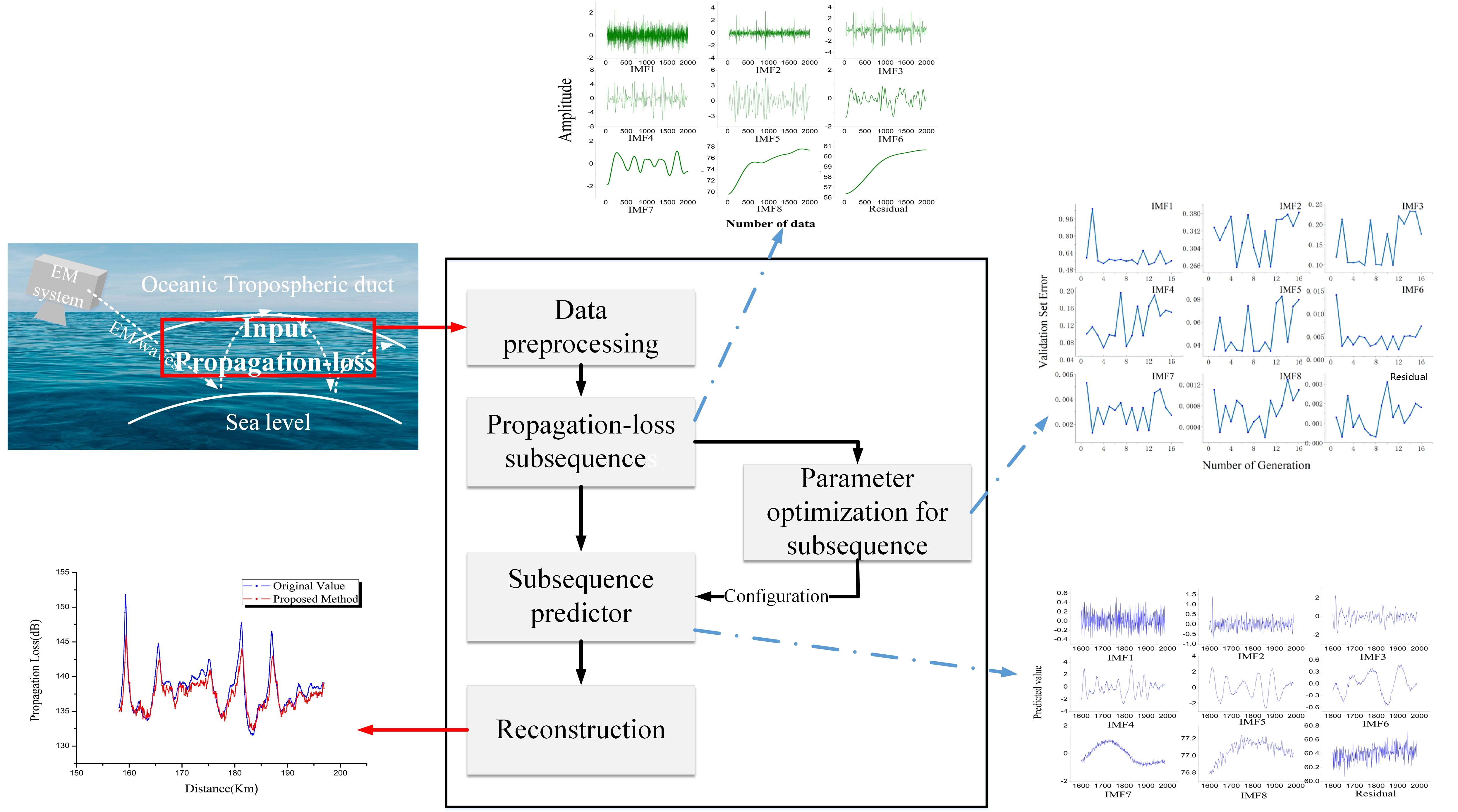
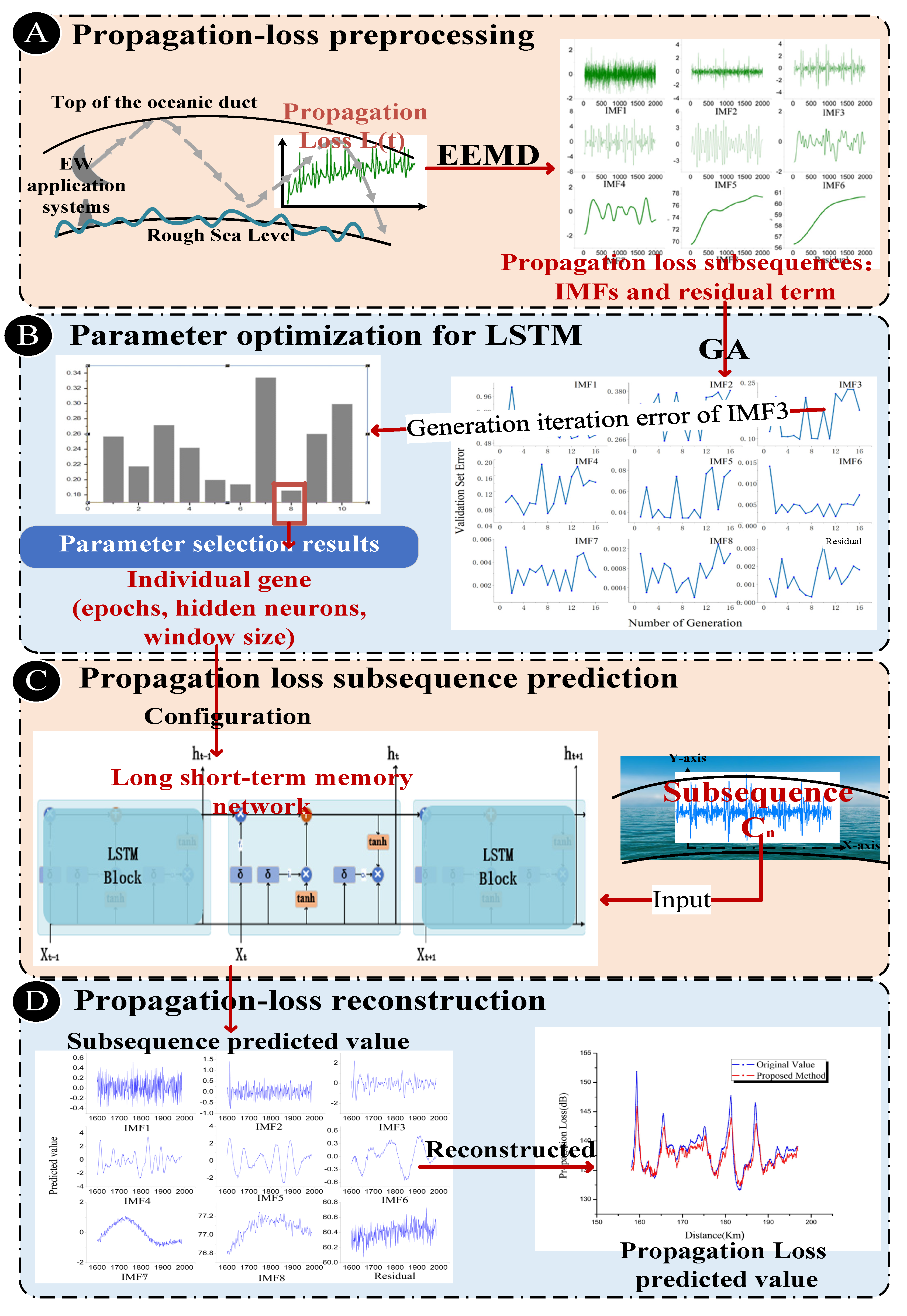
2.1. Overall Structure of the Proposed Propagation-Loss-Prediction Method

The propagation loss of EM waves in an oceanic duct is an important factor for studying the effects of oceanic ducts on the remote sensing of EM equipment. The propagation loss of EM waves in an oceanic duct consists of two parts. One part is the propagation loss in the free space. A free space is an isotropic ideal medium that does not absorb energy. Free-space propagation loss is the natural loss of energy caused by the energy diffusion of spherical waves as the propagation distance increases. The second part is the propagation loss of the medium, which is caused by the absorption of EM waves by the medium and the scattering, reflection, and diffraction of EM waves by obstacles. If the propagation in free space is denoted as $L_f$ and the propagation loss of the medium as $A$, the original propagation loss ($L(t)$) in the oceanic duct can be expressed as

$$L\left(t\right)=L_f+A$$

(1)

The framework of the proposed method of predicting propagation loss in oceanic ducts is shown in Figure 2. The EM waves are trapped in an oceanic duct layer, and the detailed propagation-loss prediction steps are described as follows:

A.

Propagation-loss preprocessing. As a data preprocessing method, EEMD decomposes the original propagation loss sequence ($L(t)$) into a limited number of subsequences $C_n$ called IMFs; and the last IMF is the residual term $Residual$:

$$L\left(t\right)={\sum }_{i=1}^N{C}_n={\sum }_{i=1}^{N-1}IM{F}_n+Residual,$$

(2)

N represents the total number of propagation loss subsequences. Meanwhile, the EEMD reduces noise and stabilizes the propagation-loss sequence.

B.

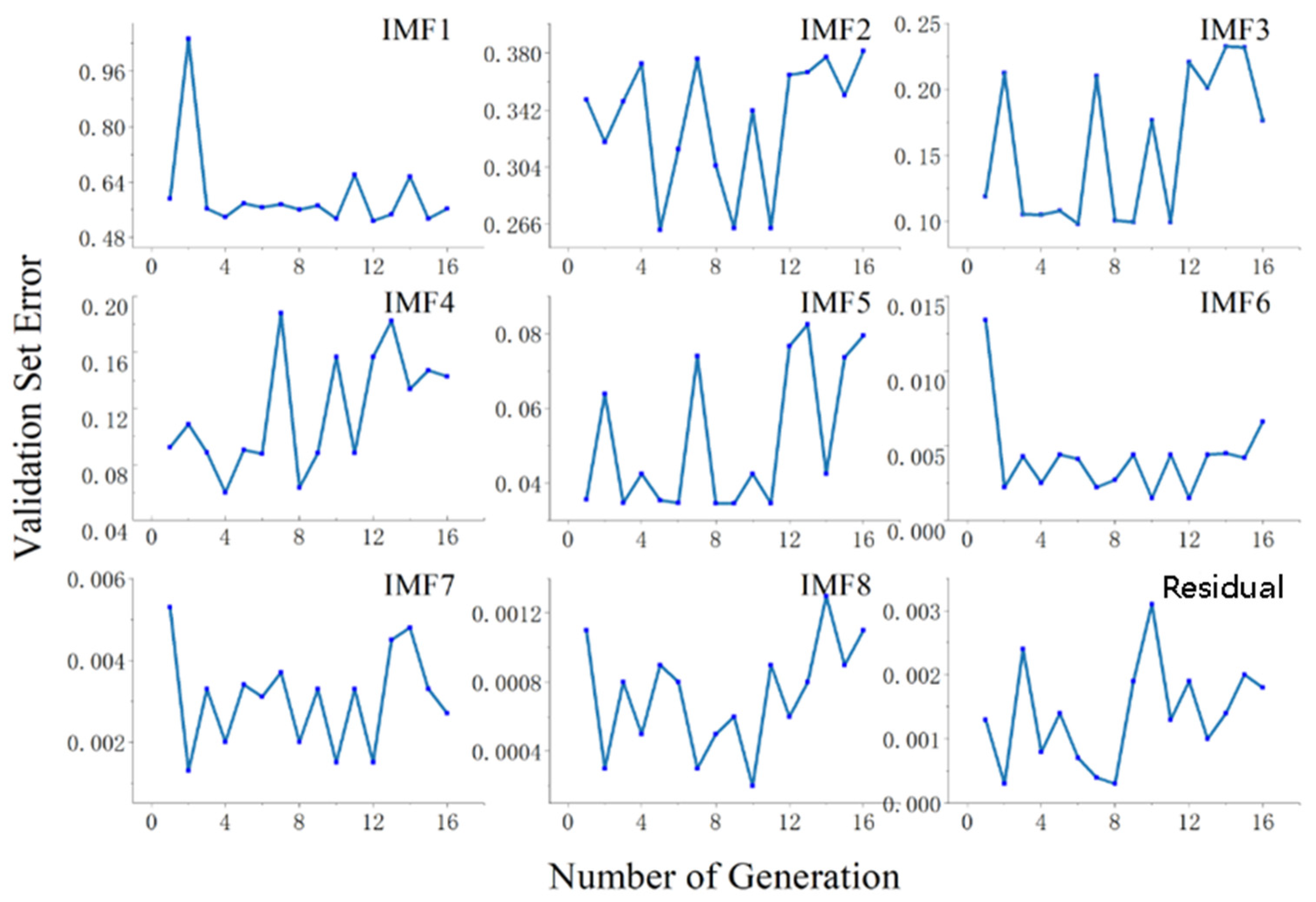
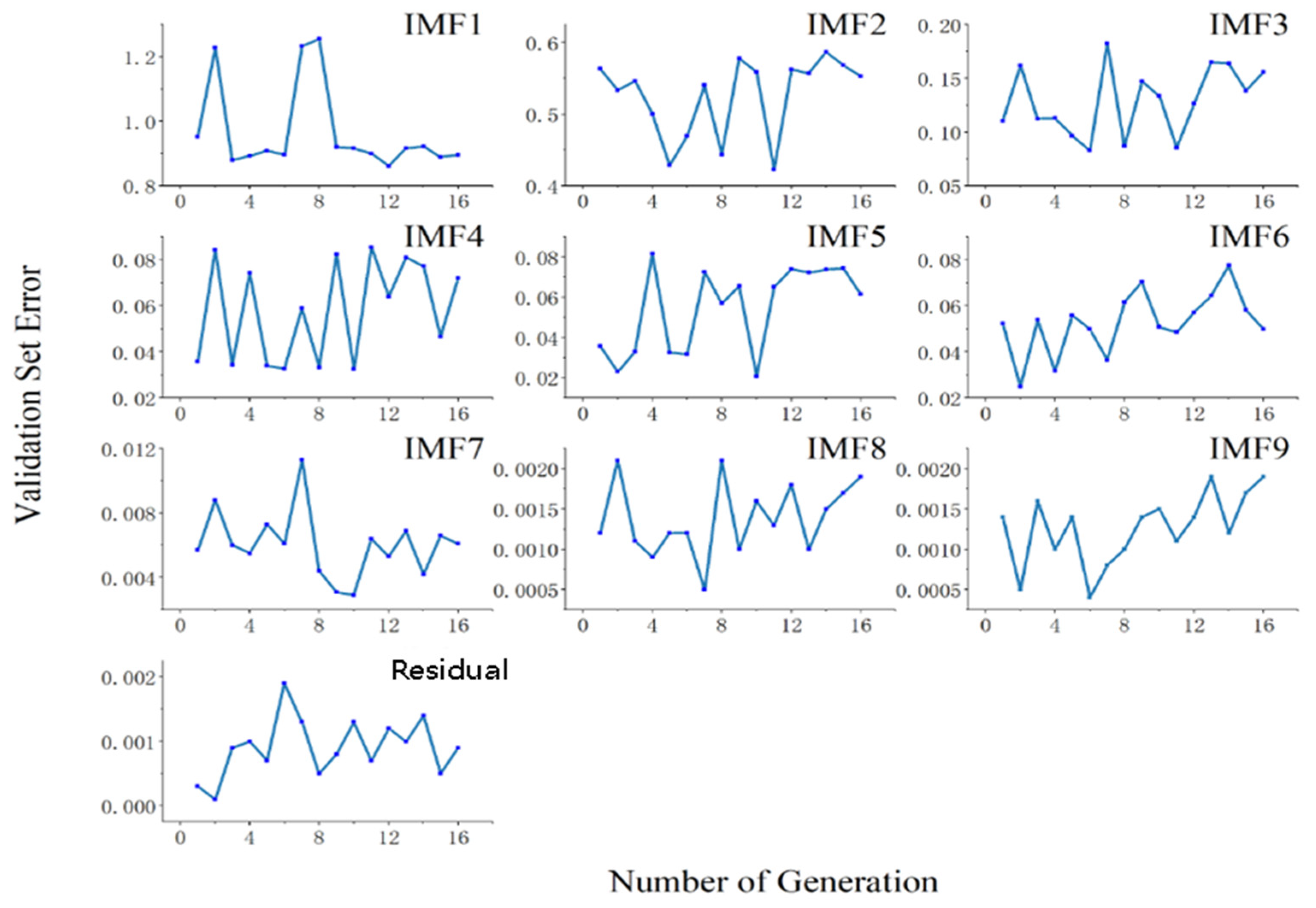
Parameter optimization for LSTM. A GA optimizes the parameters (i.e., epochs, hidden neurons, and window size) of the corresponding LSTM network according to each IMF. The GA generates chromosomes based on the optimized parameters. According to the fitness function and termination conditions (maximum number of iterations), the final output chromosome is the optimal parameter for each LSTM NN. The equation for the fitness function is as follows:

$$\mathrm{fitness}=\sqrt{\frac{1}{H}{\sum }_{j=1}^h{(y_j^{real}-y_j^{pred})}^2},$$

(3)

where $H$ represents the size of the validation set, $y_j^{real}$ and $y_j^{pred}$ are the true value and corresponding predicted value of the $j-\mathrm{th}$ propagation loss in the verification set, respectively.

C.

Propagation loss subsequence prediction. The optimized LSTM NN learns the changing laws of each subsequence through three gates: input, forget, and output gates. The gate is a fully connected layer in which the input is a subsequence vector, and the output is a real vector between 0 and 1. The equation is

$$gate\left(x\right)=\delta \left(Wx+b\right),$$

(4)

where x is the input subsequence vector, W is the weight vector, b is the bias term, δ is the activation function, and gate(x) is the corresponding output. The final subsequence prediction value is provided by the output gate.

D.

Propagation-loss reconstruction. The prediction results of each IMF and residual term are reconstructed according to Equation (5), and the final prediction results of the EM wave propagation loss in the oceanic duct are obtained:

$${\mathrm{PropagationLoss}}^{\mathrm{predicted}}={\sum }^{ }{IMF}^{\mathrm{predicted}}{ +Residual}^{\mathrm{predicted}}.$$

(5)

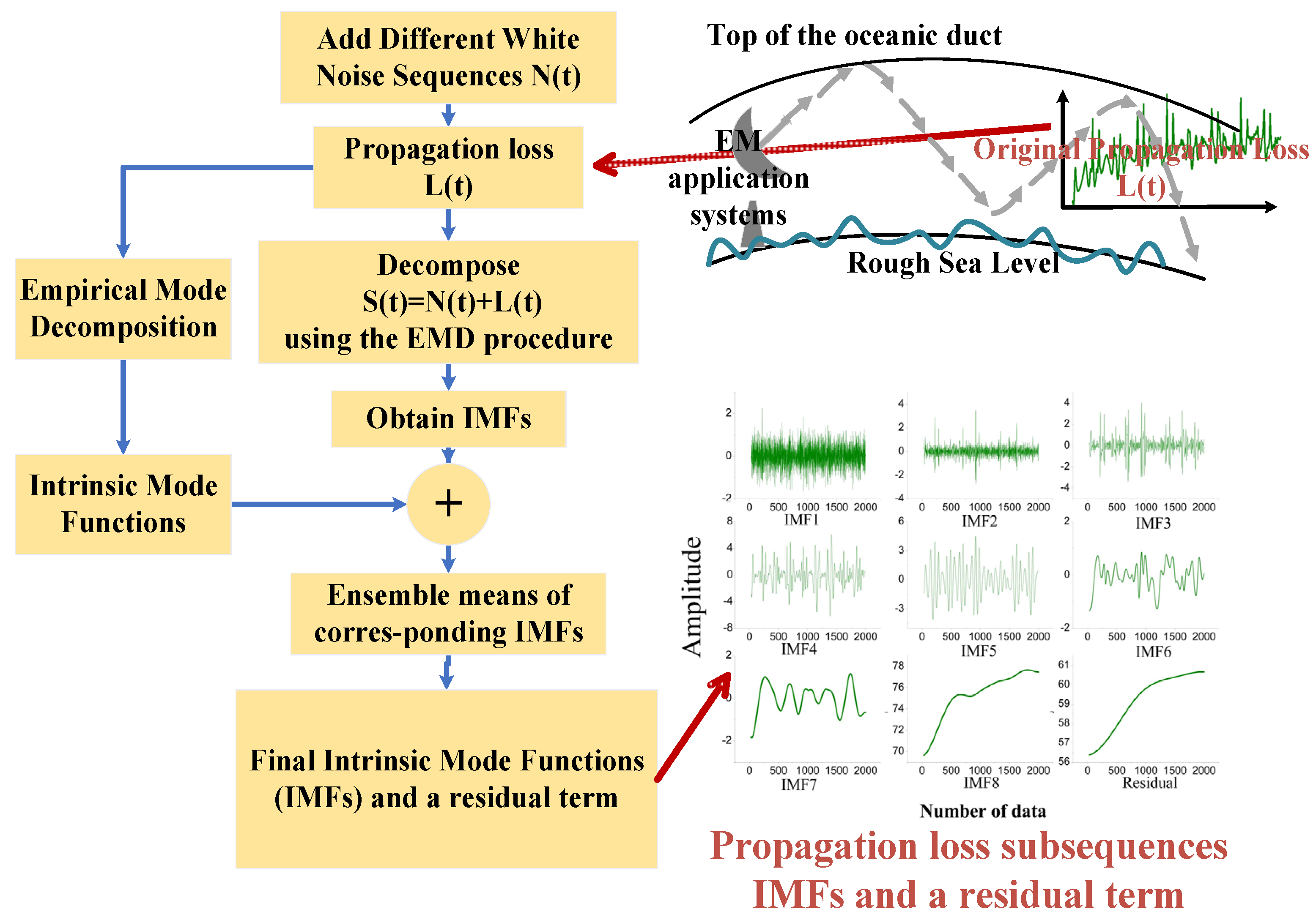
2.2. Propagation-Loss Preprocessing

An at-sea EM application system emits EM waves that are trapped in the oceanic duct layer. EM waves inevitably experience losses during the propagation process. This is caused by the natural diffusion of EM waves with distance, the absorption of media, and the refraction and scattering by obstacles in the propagation space. In other words, the EM wave propagation loss in an actual oceanic duct is a multivariate nonlinear function composed of EM system parameters (for example, emission frequency, polarization mode, and emission angle), marine environment parameters, and noise signals. In actual large-scale sea areas, the marine environmental factors that cause EM wave propagation loss change gradually and randomly. The original EM wave propagation-loss sequence is a nonlinear and nonstationary signal. Therefore, we propose EEMD [41] as a data preprocessing method. EEMD is an adaptive signal time-frequency analysis method. It autonomously extracts the IMFs and a residual term of the signal based on the characteristics of the propagation loss signal. This method is suitable for analyzing nonlinear and nonstationary signals. According to the characteristics of the original propagation loss sequence, EEMD can adaptively decompose the propagation-loss sequence into a limited number of IMFs while reducing noise and maintaining data stability. Each IMF component decomposed by EEMD contains the local characteristic signals of different time scales of the original propagation loss. The propagation-loss preprocessing is shown in Figure 3.

EEMD is a method of preprocessing propagation-loss data that introduce white noise sequences into the original propagation-loss sequence; owing to the characteristics of white noise (uniform spectrum distribution and zero mean), the white noise signal will be uniformly distributed in the original propagation-loss sequence, and the effect on the original propagation-loss sequence will be offset by the combination of multiple empirical modal decomposition and averaging. The specific process of preprocessing EM wave propagation-loss data in the oceanic duct is as follows, where $L(t)$ represents the original EM wave propagation-loss sequence collected

(1)

The ensemble number ($M$) (that is, the total number of white noises added to the original propagation loss sequence) and the amplitude of the added white noise sequence $N_m\left(t\right)$ are initialized. Additionally, $m=1$.

(2)

A new sequence $S_m\left(t\right)$ is created by adding the $m-\mathrm{th}$ white noise signal $N_m\left(t\right)$ to the original EM propagation-loss sequence $L\left(t\right)$, and the specific equation is as follows:

$$S_m\left(t\right)=L\left(t\right)+N_m\left(t\right),m\in \left[1,M\right],$$

(6)

(3)

The empirical mode decomposition (EMD) algorithm is applied to $S_m(t)$, which is decomposed into a set of IMFs ($im{f}_{m,n}$) and a residual term $res$ follows:

$$S_m\left(t\right)={\sum }_{n=1}^{N-1}im{f}_{m,n}+res,$$

(7)

where $im{f}_{m,n}$ is the $n-\mathrm{th}$ IMF obtained after the $S_m(t)$ is decomposed, $res$ is the corresponding residual term, and $N$ is the total number of subsequences obtained after EMD decomposition.

(4)

Steps (2) and (3) are repeated until $m$ reaches the maximum. After each new sequence $S_m(t)$ is decomposed, the set of IMFs is:

$$im{f}_{1,n},im{f}_{2,n},\dots \dots ,im{f}_{M,n}\left(n=1,2,\dots ,N-1\right),$$

(8)

(5)

Perform the set average operation on the IMFs set obtained in step (4), and the IMF components that can represent the different frequency domain characteristics of the original propagation loss sequence after data preprocessing are obtained:

$$IM{F}_n=\frac{1}{M}{\sum }_{m=1}^{M}im{f}_{m,n},$$

(9)

After the above steps, The original propagation-loss sequence $L\left(t\right)$ is decomposed into N propagation-loss subsequences $C_n(n=1,2,\dots ,N)$. The first N − 1 subsequences are called IMFs($IM{F}_n(n=1,2,\dots ,N-1)$), and the last subsequence is the residual term $Residual$, as shown in Equation (2).

2.3. Principle of Propagation-Loss Prediction

The original propagation loss is decomposed using EEMD to obtain a limited number of $IM{F}_n(n=1,2,\dots ,N-1)$ from a high to low frequency and a residual term $Residual$ ($n$ stands for the order of $IM{F}_n$). The higher the order, the lower the frequency. This means that $IM{F}_1$ represents the high-frequency characteristics of the original propagation-loss sequence, and $IM{F}_{N-1}$ represents the low-frequency characteristics. Each IMF has a corresponding physical meaning. We propose the use of an optimized LSTM network to predict the propagation-loss subsequences $C_n(n=1,2,\dots ,N)$ and obtain the corresponding prediction value. Finally, these predicted values are reconstructed to obtain the final prediction value of propagation loss in the oceanic duct. Figure 4 shows a schematic diagram of the propagation-loss subsequence prediction based on the LSTM network. The propagation-loss subsequence performs a sliding reconstruction according to the time window size (m) selected by the GA. The propagation-loss subsequence is converted to a supervised learning data pair: the input of the LSTM network ($X_t$), and the propagation-loss subsequence values at the current distance between the EM wave transmitting end and the propagation loss receiving end $t$, respectively. The LSTM NN learns the nonlinear relationship of the historical trend information of the propagation-loss subsequences and then predicts the propagation-loss subsequence value $Y_t$. $h_{t-1}$ is the historical trend information of the propagation-loss subsequence, $X_t$ is the input into the LSTM forecaster, and $Y_t$ is the prediction result. Equation (10) shows the prediction principle of the propagation-loss subsequence:

$$Y_t=f\left(X_t,h_{t-1}\right),$$

(10)

where $f(.)$ is a nonlinear model.

The LSTM NN can learn the dynamic change law of propagation loss through the characteristic information of the historical propagation-loss subsequence, primarily through three gates (forget, input, and output gates). The forget gate determines how much of the cell state at historical distance ($C_{t-1}$) is retained by the cell state at current distance ($C_t$). The input gate determines which propagation-loss subsequence characteristic information is retained in $C_t$, and the output gate controls $C_t$ to the current output value of the LSTM $Y_t$. The concrete steps of learning the dynamic change law of the propagation-loss subsequence in a gated unit are as follows.

1.

The first step is activating the forget gate ($f_t$), and $f_t$ determines which information of the propagation-loss characteristics will be discarded from $C_t$:

$$f_t=\delta \left(W_f\ast \left[h_{t-1},X_t\right]+b_f\right),$$

(11)

2.

The second step is the activation of the input gate ($i_t$), which determines which characteristic information of the propagation loss will be accumulated in the cell state; the function of the input gate is realized in two steps:

$$i_t=\delta \left(W_i\ast \left[h_{t-1},X_t\right]+b_i\right),$$

(12)

$${\tilde{C}}_t=\tanh (W_c\ast \left[h_{t-1},X_t\right]+b_c),$$

(13)

3.

The cell state at current distance ($C_t$) is then updated, and the cell state at historical distance ($C_{t-1}$) is introduced to update $C_t$:

$$C_t=f_t\ast C_{t-1}+i_t\ast {\tilde{C}}_t$$

(14)

where ${\tilde{C}}_t$ is the candidate vector created by $\tanh$.

4.

Finally, the output gate ($O_t$) is activated, and the predicted output value of propagation loss subsequence at current distance ($Y_t$) primarily depends on two parts. One is that the output gate determines which parts of the output unit state are the output, and the other is to push the unit state value between −1 and 1 through the activation function ($\tanh$); subsequently, the two parts are multiplied as follows:

$$O_t=\delta \left(W_o\ast \left[h_{t-1},X_t\right]+b_o\right)$$

(15)

$$Y_t=h_t=O_t\ast \tanh (C_t),$$

(16)

The propagation-loss subsequence is input to the corresponding LSTM predictor, which then outputs corresponding predicted value. Finally, according to Equation (5), the predicted value is reconstructed, and the prediction result of the EM wave propagation loss in the oceanic duct environment is obtained.

3. Experimental Results

3.1. Evaluation Criteria for Prediction Capacity

To fairly evaluate the prediction ability of the propagation-loss-prediction mode, the root mean square error (RMSE) and mean absolute error (MAE) were used to evaluate the prediction capacity of the propagation-loss-prediction methods from different scales. The smaller the RMSE and MAE, the better the prediction capacity of the propagation loss prediction method and the better the prediction accuracy of the propagation loss. In contrast, larger RMSE and MAE values mean that the prediction performance of the propagation-loss prediction method is poor, and the prediction accuracy is lower.

(1)

The RMSE [44] represented the deviation of the square root between the predicted propagation loss value ($y_j^{pred}$) the actual propagation loss value ($y_j^{real}$) in the total data size ratio. The specific equation is

$$RMSE=\sqrt{\frac{1}{K}{\sum }_{j=1}^K{\left(y_j^{pred}-y_j^{real}\right)}^2},$$

(17)

(2)

The MAE [44] was the average of the absolute error between $y_j^{pred}$ and $y_j^{real}$, and $K$ represents the size of the propagation loss test set. The MAE was a more general form of the average error as shown in Equation (18).

$$MAE=\frac{{\sum }_{j=1}^K\left|y_j^{pred}-y_j^{real}\right|}{K},$$

(18)

(3)

To analyze the prediction ability improvement of the proposed method, the improvement percentage of the evaluation index was proposed; $P_{RMSE}$ and $P_{MAE}$ represented the improvements in RMSE and MAE, respectively. These indicators are defined as follows:

$$P_{RMSE}=\frac{\left|PMS{E}_1-RMS{E}_2\right|}{RMS{E}_1}\ast 100\%,$$

(19)

$$P_{MAE}=\frac{\left|MA{E}_1-MA{E}_2\right|}{MA{E}_1}\ast 100\%,$$

(20)

3.2. Experimental Data Set

The oceanic duct types that affect radar remote sensing and communication equipment are primarily evaporation and surface ducts. To verify the prediction capability of the proposed EM wave propagation-loss-prediction method for an oceanic duct environment, the simulation hypothesis of this study is as follows: frequency= 10 GHz, Gauss antenna type, beamwidth = 0.4°, elevation = 0.0°, horizontal polarization. The lower boundary of the oceanic duct was set as the impedance boundary with a complex dielectric constant of (70.0,9i). The simulation conditions included Gaussian white noise. The sampling range of the experimental dataset was between 3 and 200 km from the signal transmitting end, with a sampling interval of 100 m and a total of 1970 propagation-loss data. The dataset of propagation loss in an oceanic evaporation duct environment was denoted as sequence 1, and that of a surface duct environment was denoted as sequence 2. In each propagation loss series, the first 1576 path loss values (accounting for 80% of the total data set) were used to construct and train the LSTM prediction layer of the proposed prediction method, and the remaining 394 path loss values (accounting for 20% of the total data) were used to test the prediction performance of the prediction method.

3.3. Comparison Method

To verify the predictive capacity of the proposed prediction method fairly, we compared it with six comparison methods: the BP, RNN, gated recurrent unit (GRU), LSTM, GA–LSTM, and EEMD–LSTM methods.

1.

BP method

The BP algorithm is a multi-layer feed-forward neural network trained according to the error back propagation algorithm [45]. The BP comparison method represents a comparison with a basic deep learning algorithm.

2.

RNN method

The traditional RNN is a commonly used sequential prediction method. It enables the network to describe the dynamic performance of the system through delay recursion [33]. This is to compare the learning abilities of the long-term rules.

3.

GRU method

The GRU is a variant of the LSTM neural network [46]. It combines the forget and output gates in the LSTM neural network into a new gate called the update gate [47]. Thus, GRU has fewer parameters and faster training speed. The comparison with the GRU method involves comparing the predictive capacity of the LSTM neural network and its variants.

4.

Hybrid neural network method

The GA–LSTM and EEMD–LSTM hybrid neural networks exhibited an improvement in the prediction performance of the propagation-loss prediction method proposed in this paper.

3.4. Optimization of the LSTM Prediction Layer

This section discusses the hyperparameter optimization of the LSTM prediction layer of the proposed method. A GA was used to optimize the three high-frequency hyperparameters (namely, number of epochs, number of hidden neurons, and window size). First, the GA randomly generated the initial population of chromosomes composed of the three hyperparameters according to the restriction conditions. The RMSE was used as an individual fitness evaluation function, and the GA operations (selection, mutation, and crossover) simulated the rule of natural superiority after several generations until the number of generations reached the stopping criterion. Finally, the chromosome with the best fitness index was used to configure the LSTM NN. Figure 5 shows that in the oceanic evaporation duct environment, the validation-set RMSE of the subsequence of propagation-loss 1 changed with the generated iteration times. Figure 5 also shows that the trend of the validation-set RMSE fluctuated at the beginning, and after the validation-set RMSE attained its minimum value, the overall trend was to increase and become stable. This also indicated that when the GA was used to optimize the hyperparameter of the proposed propagation-loss-prediction method, more was not always better for the generated iteration number.

Figure 6 shows the change trend of the valid RMSE of the subsequence (propagation-loss sequence 2) with the number of generated iterations in the surface duct environment. In addition, after the RMSE reached the minimum value, it exhibited a steady upward trend.

According to the above analysis, the hyperparameter selection results of each LSTM predictor under the oceanic evaporation duct (sequence 1) and surface duct (sequence 2) are shown in

Table 1. Result of hyperparameter optimization based on the genetic algorithm (GA).

Propagation-Loss Subsequence Evaporation Duct	Epochs	Hidden Neurons	Windows Size	Propagation-Loss Subsequence Surface Duct	Epochs	Hidden Neurons	Windows Size
IMF1	815	5	1	IMF1	987	1	1
IMF2	331	1	3	IMF2	987	1	5
IMF3	663	2	1	IMF3	663	1	5
IMF4	1554	1	5	IMF4	392	1	5
IMF5	987	1	5	IMF5	987	1	5
IMF6	392	5	1	IMF6	663	2	1
IMF7	751	2	1	IMF7	392	5	1
IMF8	1154	4	1	IMF8	1554	2	1
Residual	751	4	1	IMF9	815	5	3
				Residual	392	5	1

.

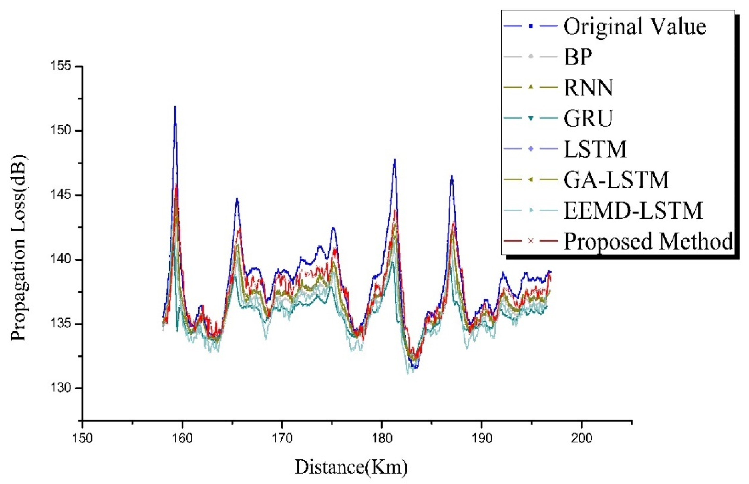
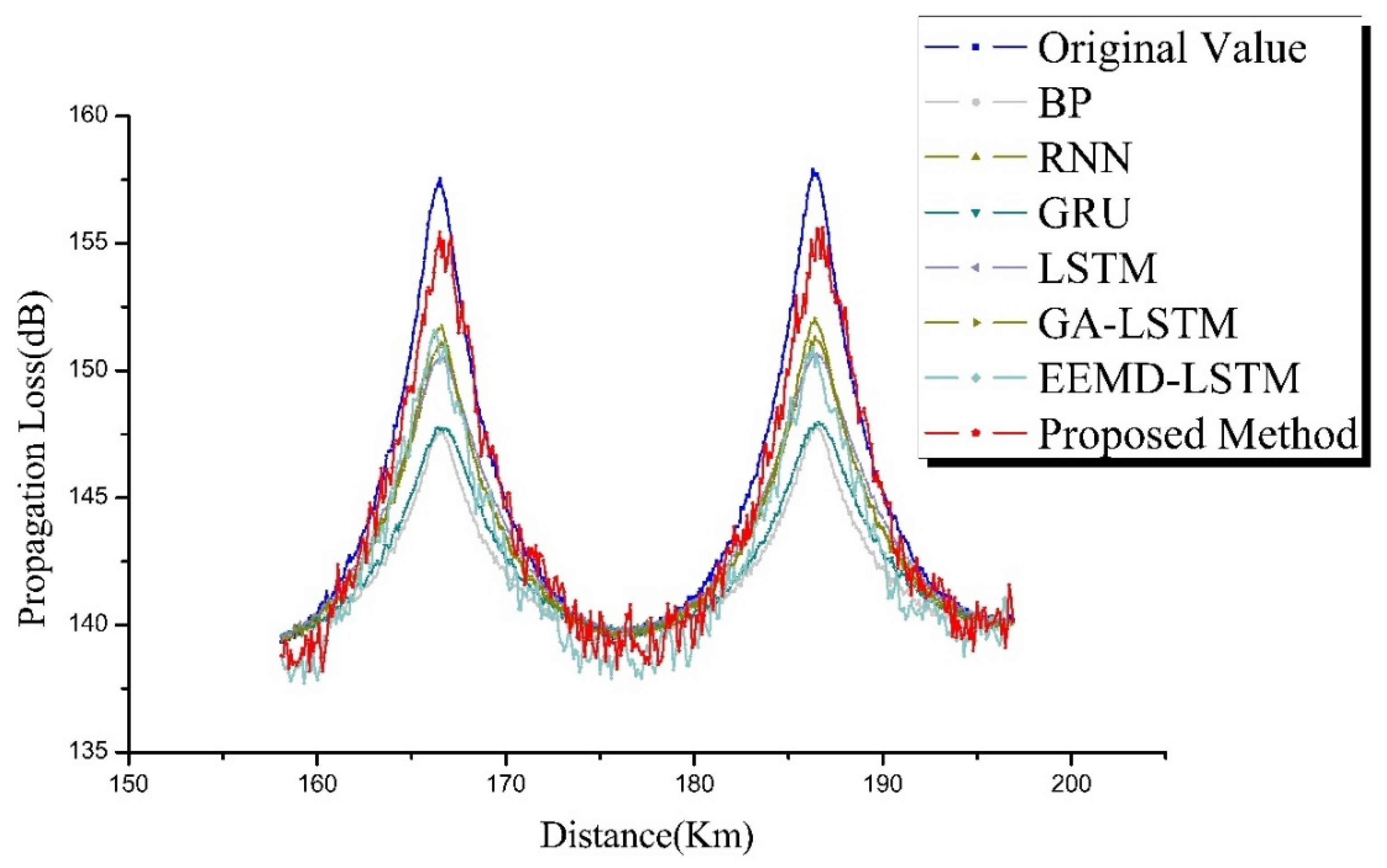
3.5. Propagation Loss Prediction Results

To verify the prediction capability of the EM wave propagation-loss prediction method for an oceanic tropospheric duct environment proposed in this paper, we applied the abovementioned six comparison methods and the proposed prediction method to the propagation loss sequences (sequences 1 and 2) in two different oceanic duct environments (evaporation duct and surface duct). Figure 7 shows a comparison of the prediction performance of all propagation-loss prediction methods on the test set of sequence 1. The evaluation index results of the prediction ability of different propagation loss prediction methods on the propagation loss of the sequence 1 test set are shown in

Table 2. Evaluation results of predictive capacity (evaporation duct).

Prediction Approaches	RMSE	MAE
BP	1.1163	0.8969
RNN	1.0636	0.8492
GRU	1.0315	0.7486
LSTM	0.8836	0.6646
GA–LSTM	0.4220	0.2790
EEMD–LSTM	0.5288	0.4577
Proposed method	0.3304	0.2683

.

Figure 8 shows the comparison of the prediction performance of all propagation-loss prediction methods on the sequence 2 test set. Similarly,

Table 3. Evaluation results of predictive capacity (surface duct).

Prediction Approaches	RMSE	MAE
BP	1.3030	0.8849
RNN	1.2333	0.8274
GRU	1.0455	0.7865
LSTM	0.7842	0.3734
GA–LSTM	0.4594	0.3127
EEMD–LSTM	0.5256	0.5014
Proposed method	0.3140	0.2613

shows the performance of different propagation loss prediction methods on the evaluation index of sequence 2.

4. Results Analysis and Discussion

4.1. Simulation Data

(a)

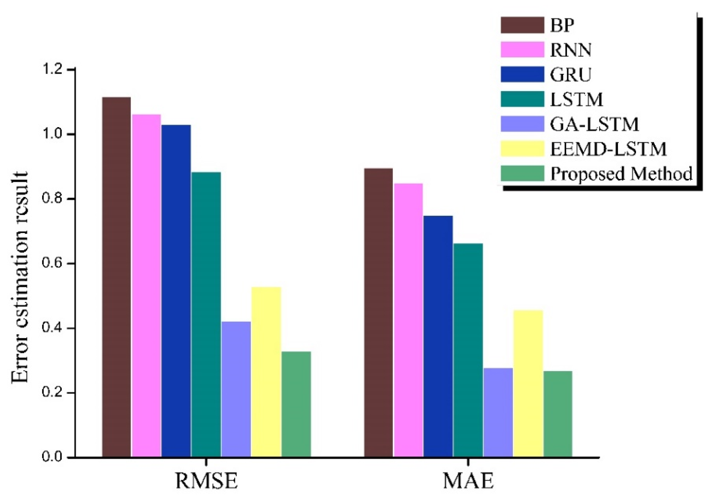
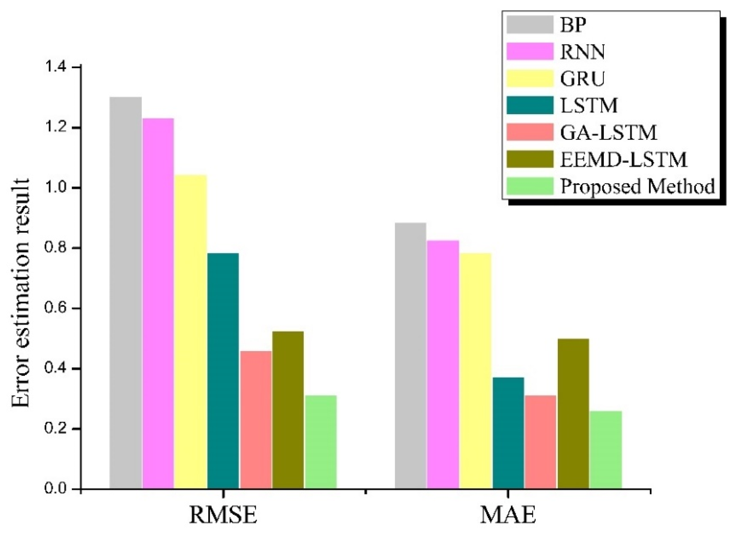
The proposed method exhibited an optimal prediction ability for propagation loss for an oceanic tropospheric duct environment.

As

Table 4. Percentage improvements of the proposed method in comparison with the other approaches on propagation loss sequence 1 (evaporation duct).

Prediction Approaches	${\mathit{P}}_{\mathit{R}\mathit{M}\mathit{S}\mathit{E}}$	${\mathit{P}}_{\mathit{M}\mathit{A}\mathit{E}}$
BP	57.41%	70.47%
RNN	74.54%	68.42%
GRU	69.97%	66.78%
LSTM	59.96%	30.02%
GA–LSTM	31.65%	16.44%
EEMD–LSTM	40.26%	47.89%

shows, for the propagation loss predictions for the evaporation duct environment, the proposed method had a higher propagation-loss prediction accuracy than the other comparison methods; for instance, compared with the BP, RNN, GRU, LSTM, GA–LSTM, and EEMD–LSTM methods, the percentage improvements in RMSE were 57.41%, 74.54%, 69.97%, 59.96%, 31.65%, and 40.26%, respectively; and the percentage improvements in the MAE were 70.47%, 68.42%, 66.78%, 30.02%, 16.44%, and 47.89%, respectively.

Table 5. Percentage improvements of the proposed method in comparison with the other approaches on propagation loss sequence 2 (surface duct).

Prediction Approaches	${\mathit{P}}_{\mathit{R}\mathit{M}\mathit{S}\mathit{E}}$	${\mathit{P}}_{\mathit{M}\mathit{A}\mathit{E}}$
BP	70.40%	70.09%
RNN	68.94%	68.41%
GRU	67.97%	64.16%
LSTM	62.61%	59.63%
GA–LSTM	21.71%	3.84%
EEMD–LSTM	37.52%	41.38%

shows the evaluation results of the prediction performance of the propagation-loss prediction method for the oceanic surface duct environment. The predictive capacity of the proposed method was superior among the six propagation loss prediction methods (i.e., BP NN, RNN, GRU, LSTM, GA–LSTM, and EEMD–LSTM). The percentage improvement of the MAE for the proposed method compared with the BP, RNN, GRU, LSTM, GA–LSTM, and EEMD–LSTM methods was 70.09%, 68.41%, 64.16%, 59.63%, 3.84%, and 41.38%, respectively. The percentage improvement of RMSE of the proposed prediction method compared with the BP, RNN, GRU, LSTM, GA–LSTM, and EEMD–LSTM methods was 70.40%, 68.94%, 67.97%, 62.61%, 21.71%, and 37.52%, respectively.

(b)

The LSTM method had a higher propagation-loss prediction accuracy than other single NN-based prediction methods.

The results in

Table 6. Percentage improvements of the LSTM method in comparison with the other single NN approaches on propagation loss sequence 1 (evaporation duct).

Prediction Approaches	${\mathit{P}}_{\mathit{R}\mathit{M}\mathit{S}\mathit{E}}$	${\mathit{P}}_{\mathit{M}\mathit{A}\mathit{E}}$
BP	20.85%	25.90%
RNN	16.92%	21.74%
GRU	14.34%	11.22%

and

Table 7. Percentage improvements of the LSTM method in comparison with the other single NN approaches on propagation loss sequence 2 (surface duct).

Prediction Approaches	${\mathit{P}}_{\mathit{R}\mathit{M}\mathit{S}\mathit{E}}$	${\mathit{P}}_{\mathit{M}\mathit{A}\mathit{E}}$
BP	39.82%	57.80%
RNN	36.41%	54.87%
GRU	24.99%	52.52%

indicate that the prediction capacity of the LSTM method was superior to that of the other single NN approaches. For the evaporation duct environment, the percentage improvement of RMSE for the LSTM method compared with the BP, RNN, and GRU approaches was 20.85%, 16.92%, and 14.34%, respectively. The percentage improvement of MAE for the LSTM method compared with the BP, RNN, and GRU approaches was 25.9%, 21.74%, and 11.22%, respectively. For the surface duct environment, the percentage improvement of RMSE for the LSTM method compared with the BP, RNN, and GRU approaches was 39.82%, 36.41%, and 24.99%, respectively. The percentage improvement of MAE for the LSTM method compared with the BP, RNN, and GRU method was 57.8%, 54.87%, and 52.52%, respectively.

(c)

The EEMD, as a data preprocessing method, effectively increased the prediction accuracy of propagation loss.

Table 8. Error estimated results of prediction approaches.

Prediction Approaches (Evaporation duct)	RMSE	MAE
LSTM	0.8836	0.6646
EEMD–LSTM	0.5288	0.4577
GA–LSTM	0.4220	0.2790
Proposed method	0.3304	0.2683
Prediction Approaches (Surface duct)	RMSE	MAE
LSTM	0.7842	0.3734
EEMD–LSTM	0.5255	0.5014
GA–LSTM	0.4594	0.3127
Proposed method	0.3140	0.2613

shows the prediction error estimated results of different propagation-loss forecast methods under two different oceanic duct environments: the LSTM-based prediction method, LSTM NN combined with parameter optimization strategy (GA–LSTM), LSTM NN hybrid data preprocessing method (EEMD–LSTM), and propagation-loss prediction method proposed in this paper.

For the evaporation duct environment, the percentage improvements of the RMSE and MAE for the EEMD–LSTM method compared with the LSTM approach, were 40.15% and 31.13%, respectively. The percentage improvements of the RMSE and MAE for the proposed method compared with the GA–LSTM approach were 9.16% and 1.07%, respectively. In the surface duct environment, the percentage improvements of the RMSE and MAE for the EEMD–LSTM method compared with the LSTM approach, were 32.99% and −34.28%, respectively. The percentage improvements of the RMSE and MAE for the proposed method compared with the GA–LSTM approach were 31.65% and 16.44%, respectively.

(d)

GA effectively increased the prediction accuracy of the propagation-loss prediction method.

Figure 9 shows the performance of the GA in increasing the propagation-loss subsequence predictive ability in the ocean evaporation duct. The GA effectively reduced the prediction error (in MAE and RMSE) of the propagation-loss subsequence predictor and improved the prediction ability of the LSTM network. The results are shown in Figure 10 for an oceanic surface duct environment.

Table 9. Percentage improvement in propagation-loss subsequences prediction capability by GA (evaporation duct).

Propagation-Loss Subsequences	${\mathit{P}}_{\mathit{R}\mathit{M}\mathit{S}\mathit{E}}$	${\mathit{P}}_{\mathit{M}\mathit{A}\mathit{E}}$
IMF1	5.25%	5.56%
IMF2	7.50%	7.42%
IMF3	7.70%	3.94%
IMF4	12.45%	9.49%
IMF5	9.04%	1.69%
IMF6	1.70%	0.93%
IMF7	36.79%	35.32%
IMF8	73.55%	75.37%
Residual	66.27%	70.47%

and

Table 10. Percentage improvement in propagation-loss subsequences prediction capability by GA (surface duct).

Propagation-Loss Subsequences	${\mathit{P}}_{\mathit{R}\mathit{M}\mathit{S}\mathit{E}}$	${\mathit{P}}_{\mathit{M}\mathit{A}\mathit{E}}$
IMF1	7.68%	8.92%
IMF2	11.80%	12.37%
IMF3	5.57%	4.71%
IMF4	3.92%	5.68%
IMF5	23.55%	22.56%
IMF6	69.82%	67.75%
IMF7	34.27%	35.25%
IMF8	19.54%	18.60%
IMF9	71.00%	72.21%
Residual	40.86%	46.78%

show the results for the percentage improvement in propagation-loss subsequence prediction capability by GA for two different oceanic ducts.

(e)

The propagation-loss prediction accuracy based on a hybrid LSTM method was higher than that of a single LSTM NN.

Table 11. Error estimation result based on the LSTM and hybrid LSTM methods.

Prediction Approaches Evaporation Duct	RMSE	MAE
LSTM	0.8836	0.6646
GA–LSTM	0.4220	0.2790
EEMD–LSTM	0.5288	0.4577
Proposed method	0.3304	0.2683
Prediction Approaches Surface Duct	RMSE	MAE
LSTM	0.7842	0.3734
GA–LSTM	0.4594	0.3127
EEMD–LSTM	0.5255	0.5014
Proposed method	0.3140	0.2613

shows the estimated results of the prediction error of the different propagation-loss forecast methods under two different oceanic duct environments. For the evaporation duct environment, the percentage improvements of the RMSE and MAE for the GA–LSTM method compared with the LSTM approach were 52.24% and 58.02%, respectively. The percentage improvements of the RMSE and MAE for the proposed method compared with the EEMD–LSTM approach were 37.52% and 41.38%, respectively. For the surface duct environment, the percentage improvements of the RMSE and MAE for the GA–LSTM method compared with the LSTM approach were 41.42% and 16.26%, respectively. The percentage improvements of the RMSE and MAE for the proposed method compared with the EEMD–LSTM approach were 40.26% and 47.89%, respectively.

(f)

Figure 11 and Figure 12 show the evaluation index results of the prediction performance of all the EM wave propagation loss-prediction methods under the oceanic evaporative duct and surface duct environments, respectively.

We observed the following: (1) among the four single intelligent propagation-loss prediction methods discussed in this paper, the LSTM method had the highest prediction accuracy; (2) compared with the single LSTM method, the forecasting capacities of the hybrid LSTM NN approaches were superior; (3) although the EEMD effectively increased the accuracy of the propagation-loss prediction, for the surface duct environment, the percentage improvement of MAE for the EEMD–LSTM method compared with the LSTM approach was −34.28%, and the percentage improvement of MAE for the proposed method compared with the EEMD–LSTM approach was 47.89%, and thus, by combining with the hyperparameter optimization algorithm of the GA, the forecasting capacity of the EEMD–LSTM was increased; and (4) compared with the other six methods, the propagation-loss prediction method proposed in this paper was superior in terms of both MAE and RMSE indices under both oceanic duct environments.

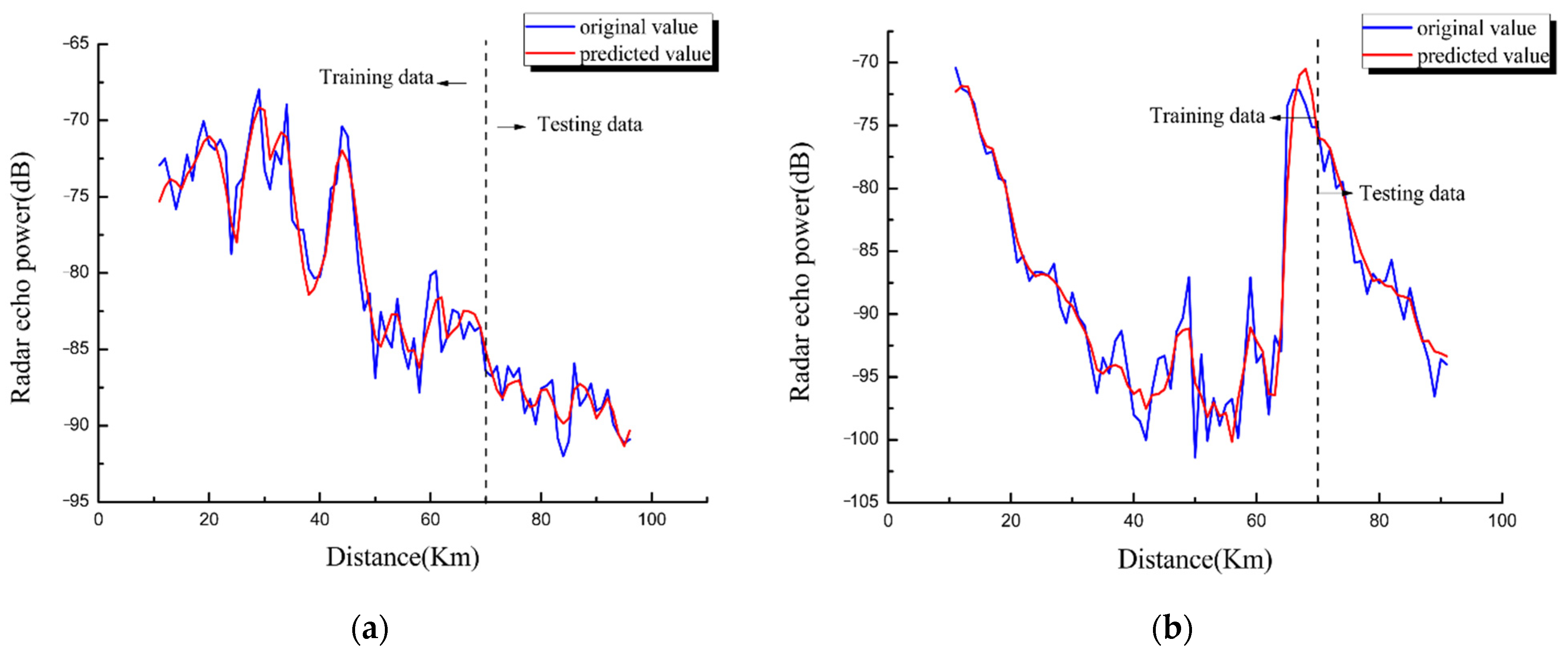
4.2. Field Data Testing

To further test the predictive performance of the proposed method in the actual oceanic duct environment, real field data was used. True doppler weather radar echoes power observation data from the observation at Qingdao Meteorological Bureau (${120}^{\circ }\mathrm{E},{36}^{\circ }\mathrm{N}$) on 18 July 2014(4:04 UTC). The corresponding field data are the two sets of radar echoes power measured in 90° and 120° azimuth (assuming that true north is 0° azimuth) in the nearby sea area (sampling approximately 1 km at distances <90 km) under a non-uniform oceanic duct environment. In the ocean duct environment, according to the basic theory of radar, the distance between the radar receiving antenna and the sea surface scattering unit is $r$, and the corresponding relationship between radar echoes power $P(r,M)$ and propagation loss $L(r)$ is as follows:

$$P\left(r,M\right)=\frac{P_t{G}^{2}4\pi A{\sigma }_0}{L{(r)}^2{\lambda }^2},$$

(21)

where $M$ is the atmospheric modified refractive index profile, $P_t$ is the transmit power of the radar, ${\sigma }_0$ is the backscatter coefficient(need to be analyzed based on sea conditions), $G$ is the radar antenna gain, and $\lambda$ is the EM wavelength. The parameters of the Doppler weather radar used are shown in

Table 12. Doppler weather radar parameters.

Radar Parameter	Value
Frequency (GHz)	3.0
Antenna elevation(degree)	0.57
Antenna height (m)	169
Transmitting power (kW)	700
Antenna gain (dB)	45
Antenna horizontal beam width (degree)	1.0
Antenna vertical beam width (degree)	1.0
Pulse width ($\mu s$)	1.0

. The relationship between the original echoes power in 90° and 120° azimuth and their prediction for the proposed method is illustrated in Figure 13, and

Table 13. Evaluation results of predictive capacity.

Prediction Approaches 90° Azimuth	RMSE	MAE
BP	3.7338	3.3076
RNN	3.2216	2.8937
GRU	3.6098	3.2750
LSTM	1.8432	1.4385
GA–LSTM	1.8323	1.4264
EEMD–LSTM	1.4729	1.1208
Proposed method	1.0644	0.8700
Prediction Approaches 120° Azimuth	RMSE	MAE
BP	4.3998	2.4776
RNN	2.8040	2.1168
GRU	2.7277	2.0772
LSTM	2.2747	1.9604
GA–LSTM	2.0859	1.7750
EEMD–LSTM	1.6657	1.3358
Proposed method	1.4515	1.0816

is the evaluation result of the prediction ability of different prediction methods on the radar echoes power testing data.

It is shown in Figure 13, when using real radar echoes power data, although the field data contains some observation deviations, the prediction results can better fit the change trend of field data, and the prediction error is between −2dB and 2dB. As Table 13 shows, for the radar echoes power field data predictions in the actual oceanic duct environment, the proposed method had a higher prediction accuracy than the other comparison methods in 90° and 120° azimuth; for instance, in 90° azimuth, compared with the BP, RNN, GRU, LSTM, GA–LSTM, and EEMD–LSTM methods, the percentage improvement in RMSE was 71.49%, 66.96%, 70.51%, 42.25%, 41.91%, and 27.73%, respectively; and the percentage improvements in the MAE was 73.70%, 69.93%, 73.43%, 39.52%, 39.00%, and 22.38%, respectively. In 120° azimuth, the percentage improvement of the MAE for the proposed method compared with the BP, RNN, GRU, LSTM, GA–LSTM, and EEMD–LSTM methods was 56.34%, 48.90%, 47.93%, 44.83%, 39.06%, and 19.03%, respectively. The percentage improvement of RMSE of the proposed prediction method compared with the BP, RNN, GRU, LSTM, GA–LSTM, and EEMD–LSTM methods was 67.01%, 48.24%, 46.79%, 36.19%, 30.42%, and 12.86%, respectively. Overall, based on the prediction results of the field data, we can see that the proposed prediction method is relatively successful.

5. Conclusions

Ocean tropospheric ducts severely affect the performance of EM systems designed for environments with normal atmospheric refraction. The oceanic duct types that affect radar performance and communication equipment are primarily the evaporation and surface ducts. Based on the simulated propagation loss data of the above two oceanic duct environments, we propose a propagation-loss prediction method based on an improved LSTM neural network. The propagation-loss prediction results were compared with six other prediction methods (i.e., BP method, RNN method, GRU method, LSTM method, and GA–LSTM and EEMD–LSTM hybrid methods), and the experimental results demonstrated that the prediction performance of the proposed method is generally better. Owing to the uncertainty, volatility, and noisy characteristics of marine environmental parameters, the EEMD method was used to predict propagation loss to extract the data characteristics of different frequencies while stabilizing the data. The error estimation results indicated that the combination with the EEMD method enables the LSTM predictor to have strong anti-noise ability and is more suitable for actual marine environments. Simultaneously, the GA can effectively improve the prediction ability of the LSTM predictor. Although a prediction error exists, the field data testing shows that the field data in the actual oceanic duct environment predicted by the proposed prediction method conforms to the changing trend of real field data.

In the future, prediction data based on the measured propagation loss can be used to predict the occurrence and strength information of the oceanic duct. It can also be used as a priori information to increase the real-time inversion accuracy of regional nonuniform oceanic ducts.

References

1. Zhang, J.P.; Wu, Z.-S.; Zhao, Z.-W.; Zhang, Y.-S.; Wang, B. Propagation modeling of ocean-scattered low-elevation GPS signals for maritime tropospheric duct inversion. Chin. Phys. B 2012, 21, 109202. [Google Scholar] [CrossRef]
2. Yang, S.; Yang, K.D.; Yang, Y.X.; Ma, Y.L. Experimental verification of effect of horizontal inhomogeneity of evaporation duct on electromagnetic wave propagation. Chin. Phys. B 2015, 24, 044102. [Google Scholar]
3. Shi, Y.; Yang, K.-D.; Yang, Y.-X.; Ma, Y.-L. Influence of obstacle on electromagnetic wave propagation in evaporation duct with experiment verification. Chin. Phys. B 2015, 24, 054101. [Google Scholar] [CrossRef]
4. Protopapadakis, E.; Voulodimos, A.; Doulamis, A.; Doulamis, N.; Dres, D.; Bimpas, M. Stacked autoencoders for outlier detection in over-the-horizon radar signals. Comput. Intell. Neurosci. 2017, 2017. [Google Scholar] [CrossRef]
5. Wagner, M.; Gerstoft, P.; Rogers, T. Estimating refractivity from propagation loss in turbulent media. J. Radio Sci. 2016, 51, 1876–1894. [Google Scholar] [CrossRef] [Green Version]
6. Ullah, A.; Rehman, S.U.; Mufti, N. Investigations into the occurrence of elevated ducts in lower atmosphere near Arabian Sea. In Proceedings of the 2015 International Conference on Space Science and Communication (IconSpace), Langkawi, Malaysia, 10–12 August 2015; pp. 128–131. [Google Scholar]
7. Rehman, S.U.; Mufti, N. Investigations into the occurrence of evaporation ducts near Karachi. In Proceedings of the 2017 International Conference on Communication Technologies (ComTech), Rawalpindi, Pakistan, 19–21 April 2017; pp. 34–38. [Google Scholar]
8. Teti, J. Parabolic equation methods for electromagnetic wave propagation [Book Review]. IEEE Antennas Propag. Mag. 2001, 43, 96–97. [Google Scholar] [CrossRef]
9. Durand, J.C.; Granier, P. Radar coverage assessment in nonstandard and ducting conditions: A geometrical optics approach. In IEE Proceedings F (Radar and Signal Processing); IET Digital Library: Wales and Scotland, UK, 1990; pp. 95–101. [Google Scholar]
10. Budden, K.G. The Wave-Guide Mode Theory of Wave Propagation; Logos Press: London, UK, 1961. [Google Scholar]
11. Levy, M. Parabolic Equation Methods for Electromagnetic Wave Propagation; No. 45. IET; Institution of Engineering and Technology (IET): London, UK, 2000. [Google Scholar]
12. Iqbal, A.; Jeoti, V. Numerical evaluation of radiowave propagation in evaporation ducts using FEM. In Proceedings of the 2011 National Postgraduate Conference, Perak, Malaysia, 19–20 September 2011; pp. 1–6. [Google Scholar]
13. Zhao, X.-F.; Huang, S.-X.; Kang, L.-C. New method to solve electromagnetic parabolic equation. Appl. Math. Mech. 2013, 34, 1373–1382. [Google Scholar] [CrossRef]
14. Bitner-Gregersen, E.M.; Bhattacharya, S.K.; Chatjigeorgiou, I.K.; Eames, I.; Ellermann, K.; Ewans, K.; Hermanski, G.; Johnson, M.C.; Ma, N.; Maisondieu, C.; et al. Recent developments of ocean environmental description with focus on uncertainties. Ocean Eng. 2014, 86, 26–46. [Google Scholar] [CrossRef]
15. Zheng, Y.Q.; Li, J.S.; Gong, L.X.; Zeng, X.M.; Gao, J.L.; Gao, Y. Characteristics of spring and summer weather over the Gulf of Aden. J. PLA Univ. Sci. Technol. 2012, 6, 688–693. [Google Scholar]
16. Liu, Y.; Zhou, X.L.; Jin, H.Q.; Wang, W.Y. Research on Influence of Rough Sea Surface on Radio Wave Propagation. J. Radio Eng. 2012, 3, 38–40. [Google Scholar]
17. Liu, Y.; Zhou, X.-L.; Pei, R.-J. Study on Rough Sea-surface Radio Wave Propagation based on PE Model. Commun. Technol. 2012, 45, 4–6. [Google Scholar]
18. Karimian, A.; Yardim, C.; Hodgkiss, W.S.; Gerstoft, P.; Barrios, A.E. Estimation of radio refractivity using a multiple angle clutter model. Radio Sci. 2012, 47, 1–9. [Google Scholar] [CrossRef]
19. Yang, S.; Yang, Y.; Yang, K. Electromagnetic Wave Propagation Simulation in Horizontally Inhomogeneous Evaporation Duct. In Theory. Methodology, Tools and Applications for Modeling and Simulation of Complex Systems; Springer: Singapore, 2016; pp. 210–216. [Google Scholar]
20. Burk, S.D.; Haack, T.; Rogers, L.T.; Wagner, L.J. Island Wake Dynamics and Wake Influence on the Evaporation Duct and Radar Propagation. J. Appl. Meteorol. 2003, 42, 349–367. [Google Scholar] [CrossRef]
21. Sheng, Z.; Wang, J.; Zhou, S.; Zhou, B. Parameter estimation for chaotic systems using a hybrid adaptive cuckoo search with simulated annealing algorithm. Chaos Interdiscip. J. Nonlinear Sci. 2014, 24, 013133. [Google Scholar] [CrossRef]
22. Zhao, X.; Huang, S. Atmospheric duct estimation using radar sea clutter returns by the adjoint method with regularization technique. J. Atmos. Ocean. Technol. 2014, 31, 1250–1262. [Google Scholar] [CrossRef]
23. Zhang, J.; Wu, Z.; Wang, B.; Wang, H.; Zhu, Q. Modeling low elevation GPS signal propagation in maritime atmospheric ducts. J. Atmos. Sol.-Terr. Phys. 2012, 80, 12–20. [Google Scholar] [CrossRef]
24. Hetherington, P.A.; Groves, A.R. System for Suppressing Rain Noise. U.S. Patent No. 7949522, 24 May 2011. [Google Scholar]
25. Rogers, L.T.; Hattan, C.P.; Stapleton, J.K. Estimating evaporation duct heights from radar sea echo. Radio Sci. 2000, 35, 955–966. [Google Scholar] [CrossRef] [Green Version]
26. De Gooijer, J.G.; Hyndman, R.J. 25 years of time series forecasting. Int. J. Forecast. 2006, 22, 443–473. [Google Scholar] [CrossRef] [Green Version]
27. Zhang, G.; Patuwo, B.E.; Hu, M.Y. Forecasting with artificial neural networks: The state of the art. Int. J. Forecast. 1998, 14, 35–62. [Google Scholar] [CrossRef]
28. Mom, J.M.; Mgbe, C.O.; Igwue, G.A. Igwue. Application of artificial neural network for path loss prediction in urban macrocellular environment. Am. J. Eng. Res. 2014, 3, 270–275. [Google Scholar]
29. Ostlin, E.; Zepernick, H.-J.; Suzuki, H. Macrocell Path-Loss Prediction Using Artificial Neural Networks. IEEE Trans. Veh. Technol. 2010, 59, 2735–2747. [Google Scholar] [CrossRef] [Green Version]
30. Cheerla, S.; Ratnam, D.V.; Borra, H.S. Neural network-based path loss model for cellular mobile networks at 800 and 1800 MHz bands. AEU Int. J. Electron. Commun. 2018, 94, 179–186. [Google Scholar] [CrossRef]
31. Popescu, I.; Nikitopoulos, D.; Constantinou, P.; Nafornita, I. ANN prediction models for outdoor environment. In Proceedings of the 2006 IEEE 17th International Symposium on Personal, Indoor and Mobile Radio Communications, Helsinki, Finland, 11–14 September 2006; pp. 1–5. [Google Scholar]
32. Hüsken, M.; Stagge, P. Recurrent neural networks for time series classification. Neurocomputing 2003, 50, 223–235. [Google Scholar] [CrossRef]
33. Bayer, J.S. Learning Sequence Representations. Ph.D. Thesis, Technische Universität München, München, Germany, 2015. [Google Scholar]
34. Pascanu, R.; Mikolov, T.; Bengio, Y. On the difficulty of training recurrent neural networks. In Proceedings of the International Conference on Machine Learning, Atlanta, GA, USA, 16–21 June 2013; pp. 1310–1318. [Google Scholar]
35. Hochreiter, S.; Schmidhuber, J. Long Short-Term Memory. Neural Comput. 1997, 9, 1735–1780. [Google Scholar] [CrossRef]
36. Li, Q.; Yin, Z.Y.; Zhu, X.Q.; Zhang, Y.S. Measurement and Modeling of Radar Clutter from Land and Sea; National Defense Industry Press: Beijing, China, 2017; p. 16. [Google Scholar]
37. Ma, L.; Wu, Z.; Zhang, J.; Jeon, G.; Tan, M. Sea Clutter Amplitude Prediction Using a Long Short-Term Memory Neural Network. Remote Sens. 2019, 11, 2826. [Google Scholar] [CrossRef] [Green Version]
38. Poli, P.; Hersbach, H.; Dee, D.P.; Berrisford, P.; Simmons, A.J.; Vitart, F.; Laloyaux, P.; Tan, D.G.H.; Peubey, C.; Thépaut, J.-N.; et al. ERA-20C: An Atmospheric Reanalysis of the Twentieth Century. J. Clim. 2016, 29, 4083–4097. [Google Scholar] [CrossRef]
39. Wu, Z.; Huang, N.E. Ensemble empirical mode decomposition: A noise-assisted data analysis method. Adv. Adapt. Data Anal. 2009, 1, 1–41. [Google Scholar] [CrossRef]
40. Liu, D.; Niu, D.; Wang, H.; Fan, L. Short-term wind speed forecasting using wavelet transform and support vector machines optimized by genetic algorithm. Renew. Energy 2014, 62, 592–597. [Google Scholar] [CrossRef]
41. Liu, H.; Mi, X.; Li, Y. Smart deep learning-based wind speed prediction model using wavelet packet decomposition, convolutional neural network and convolutional long short-term memory network. Energy Convers. Manag. 2018, 166, 120–131. [Google Scholar] [CrossRef]
42. Liu, W.; Liu, Q.; Ruan, F.; Liang, Z.; Qiu, H. Springback prediction for sheet metal forming based on GA-ANN technology. J. Mater. Process. Technol. 2007, 187–188, 227–231. [Google Scholar] [CrossRef]
43. Wang, S.; Zhang, N.; Wu, L.; Wang, Y. Wind speed forecasting based on the hybrid ensemble empirical mode decomposition and GA-BP neural network method. Renew. Energy 2016, 94, 629–636. [Google Scholar] [CrossRef]
44. Hyndman, R.J.; Koehler, A.B. Another look at measures of forecast accuracy. Int. J. Forecast. 2006, 22, 679–688. [Google Scholar] [CrossRef] [Green Version]
45. Sadeghi, B. A BP-neural network predictor model for plastic injection molding process. J. Mater. Process. Technol. 2000, 103, 411–416. [Google Scholar] [CrossRef]
46. Chen, J.; Jing, H.; Chang, Y.; Liu, Q. Gated recurrent unit based recurrent neural network for remaining useful life prediction of nonlinear deterioration process. Reliab. Eng. Syst. Saf. 2019, 185, 372–382. [Google Scholar] [CrossRef]
47. Greff, K.; Srivastava, R.K.; Koutnik, J.; Steunebrink, B.R.; Schmidhuber, J. LSTM: A Search Space Odyssey. IEEE Trans. Neural Netw. Learn. Syst. 2017, 28, 2222–2232. [Google Scholar] [CrossRef] [Green Version]
Figure 1. Propagation of electromagnetic waves in an oceanic duct layer.
Remotesensing 13 01173 g001
Figure 2. Flow chart of predicting propagation loss. (A) propagation-loss preprocessing; (B) parameter optimization for LSTM; (C) propagation-loss subsequence prediction; (D) propagation-loss reconstruction.
Remotesensing 13 01173 g002
Figure 3. Preprocessing of propagation loss in an oceanic tropospheric duct based on ensemble empirical mode decomposition (EEMD).
Remotesensing 13 01173 g003
Figure 4. Propagation-loss subsequence predictor based on long short-term memory (LSTM).
Remotesensing 13 01173 g004
Figure 5. Propagation-loss subsequence validation set error and generated iteration (evaporation duct).
Remotesensing 13 01173 g005
Figure 6. Propagation-loss subsequence validation set error and generated iteration (surface duct).
Remotesensing 13 01173 g006
Figure 7. Comparison result of prediction performance of all prediction approaches (evaporation duct).
Remotesensing 13 01173 g007
Figure 8. Comparison result of prediction performance of all prediction approaches (surface duct).
Remotesensing 13 01173 g008
Figure 9. Error estimate results for propagation-loss subsequences in an oceanic evaporation duct: (a) root mean square error (RMSE); (b) mean absolute error (MAE).
Remotesensing 13 01173 g009
Figure 10. Error estimate results for propagation-loss subsequences in an oceanic surface duct: (a) root mean square error (RMSE); (b) mean absolute error (MAE).
Remotesensing 13 01173 g010
Figure 11. Error estimation result of propagation-loss prediction methods (evaporation duct).
Remotesensing 13 01173 g011
Figure 12. Error estimation result of propagation-loss prediction methods (surface duct).
Remotesensing 13 01173 g012
Figure 13. The radar echoes power predicted result of the proposed method: (a) 90° azimuth; (b) 120° azimuth.
Remotesensing 13 01173 g013