Abstract
Analyzing the spatiotemporal characteristics and causes of landscape pattern changes in watersheds around big cities is essential for understanding the ecological consequence of urbanization and provides a basic reference for the watershed management. This study used a land-use transition matrix and landscape indices to explore the spatiotemporal change of land use and landscape pattern over Liuxihe River basin of Guangzhou in the southeast of China from 1980 to 2015 with multitemporal Landsat satellite data in response to the rapid urbanization process. Primary temporal and spatial influencing factors were first quantitatively identified through grey relation analysis (calculating correlation degree between land use changes and influencing factors) and Geodetector (detecting landscape spatial heterogeneity and its driving factors), respectively. Considerable spatial and temporal differences in land use and landscape pattern changes were observed herein, thus determining the influencing factors of these differences in the Liuxihe River basin. These changes were characterized by a large increase in construction land converted from cropland, particularly in the middle and lower reaches of the basin from 2000 to 2010, causing dramatic fragmentation and homogenization of the landscape pattern there. Meanwhile, the landscape pattern gradually transitioned from an agricultural land use dominant landscape to a construction land use dominant landscape in these regions. Furthermore, the rapid growth of a nonagricultural population and the transformation of industry primarily caused the temporal changes of landscape pattern, and the landscape spatial heterogeneity was mainly caused by the interaction of complicated geomorphology and anthropogenic activities in different spatial locations, particularly after 2000. This study not only provides an improved approach to quantifying the main spatiotemporal influencing factors of landscape pattern changes during different time periods, but also offers a reference for decision-makers to formulate optimal strategies on ecological protection and urban sustainable development of different regions in this study area.
1. Introduction
The increasing expansion of big cities has been a common social and economic phenomenon taking place all around the world, especially in the developing countries since the 21st century [1,2]. This process, with no sign of slowing down, may be the most critical anthropogenic force that has brought about dramatic changes in land use and landscape pattern at local, regional, and global scales [3,4,5]. Numerous studies have found that these immense changes can not only contribute to various environmental issues [6,7], but also affect the structure, function, and health of the ecosystem [8,9], and further threaten the sustainable development of big cities [10,11]. Therein, watersheds around rapidly urbanizing areas are more sensitive to these changes due to its richer and fragile natural ecosystems [12]. Moreover, a watershed is a complete natural and unnatural circulation unit, which is more conducive to conduct the ecological protection and restoration. The problem related to landscape pattern changes in these kinds of watersheds has been receiving more and more attention from international scholars in recent decades [13,14]. Therefore, gaining a deep understanding of the processes and causes of landscape pattern changes is crucial for protection, management, and sustainable planning of these areas under rapid urbanization [15,16].
Previous studies have illustrated that the analysis of land use changes is usually regarded as the basis for studying the landscape patterns change [17], because the landscape pattern is usually defined as the spatial arrangement of various landscape patches of different types, sizes, and shapes, which are classified by different land use types [18]. Changes in the landscape pattern were proved to be the results of changes in various land use types [19]. Most scholars choose a land use transition matrix to reflect the mutual transformation characteristics between any two different land use types [20,21], and use landscape metrics to detect the characteristics of spatial-structural composition and configuration in different landscape patches [22,23]. Therein, the former emphasizes changes of land surface properties in different periods [24], and the latter stresses the changes of potential ecological pattern [25]. When studying the changing characteristics of landscape pattern, it is necessary to analyze land use changes first, and emphasize both the temporal and spatial changes of them.
Currently, previous studies on the change of watershed landscape pattern in rapidly urbanizing areas seldom quantified spatiotemporal processes and causes of landscape pattern changes comprehensively. For example, Su et al. [26] analyzed the land use and landscape pattern in a different period to reflect its spatiotemporal changes characteristics and its causes, but ignored the overall spatial heterogeneity of landscape pattern. Zhang et al. [27] and Shi et al. [28] systematically analyzed the spatiotemporal changes processes of land use and landscape pattern in watersheds. The former study only quantified the temporal influencing factors of land use changes, and the latter study described the temporal and spatial influencing factors respectively, but not quantitatively. In addition, when analyzing the influencing factors of landscape pattern changes quantitatively, many studies failed to solve the problem of insufficient multi-temporal land use data [29,30,31], nor did they consider the interactive effects of different factors on the spatial landscape heterogeneity [32,33]. Some studies even analyzed the transition driving forces of different land use types in different locations of different period to meet the requirements of large quantities data for commonly used analysis methods [34]. But the causes of the spatial characteristics of landscape pattern were ignored in this case. Considering the fact that the analysis of both spatial and temporal causes were all important for guiding the management and protection of the natural ecosystem in watershed [35]. There is no doubt that researchers should carry out a systematic analysis on the process and cause of watershed landscape pattern spatiotemporal changes quantitatively.
With the continuous improvement of the remote sensing technology, more and more remote sensing data with different sensors, time periods, spectrum and spatial resolution can be acquired [36]. It provides the most stable and accurate multi-temporal data source for land use analysis, thus the land use and landscape pattern changes under the rapid urbanization can be monitored and analyzed spatiotemporally [37]. There existed many studies that using these kinds of data analyzed the land use change of different regions in Guangzhou city [38,39], and compared the relationships between these changes and urban expansion [40,41]. Liu et al. [31] also discussed the land use change and its causes based on the Landsat satellite data with remote sensing technology. These researches all illustrated the feasibility of using land use data provided by remote sensing technology to analyze the changes of landscape patterns in Guangzhou city. Besides, along with the rapidly urban expansion of Guangzhou city, the intensive interaction between natural and human elements in the LXH has brought about the large transition of construction land from lots of forest and cropland [42]. The water quality and natural environment of the LXH were degraded, especially in the downstream [43,44]. The Liuxihe River basin (LXH), as the final ecological barrier on the northwest of Guangzhou city, is an important water resource conservation area. Therefore, compared with areas divided by the administrative units in Guangzhou city, analyzing the landscape pattern changes in the LXH has greater ecological significance and protection value for Guangzhou.
This study mainly analyzes the spatiotemporal differences of process and causes on landscape pattern changes under rapid urbanization of the Guangzhou city. The specific objectives are: (1) To analyze the changes of different land use types in time and space; (2) to characterize the spatial configuration of the landscape pattern in time and space; (3) to establish the relationship between changes in different land use types and different influencing factors temporally; and (4) to determine the impact of different factors on the landscape heterogeneity. Thus, these differences in the spatiotemporal changes and causes of landscape pattern in the LXH under the rapid urbanization since 1980 are revealed. The decision-makers will be more clear about how to formulate an appropriate strategy for planning and management.
2. Materials and Methods
2.1. Study Area
The Liuxihe River basin is in the rapidly developing and urbanizing city of Guangzhou, southeast of China (Figure 1). The river, about 171 km in length with an area of 2300 km2, flows through Guangzhou, and eventually empties into the Beijiang River, a tributary of the Pearl River. The annual precipitation rate over the LXH is 1750 mm and more than 80% of precipitation occurs from April to September. Its daily mean air temperature is about 20 °C and annual rate of evaporation is about 1200 mm [45]. The elevation of the LXH falls gradually from northeast to southwest, characterized by mountains in the upstream, hills in the midstream, and plains in the downstream, thus making the upstream more difficult to develop than the middle and lower watershed. At present, the distribution of land use in the LXH is characterized by forests in the upstream, croplands and orchards in the midstream, and construction lands in the downstream. In addition, the speed of the urbanization process in the midstream and downstream of the LXH is faster and stronger than in the upstream [46]. The special location conditions, the unbalancing effect of urbanization, the difference in natural topography, and the land uses/land covers all make the LXH an appropriate case for the research processes and influencing factors for spatiotemporal changes of watershed landscape pattern in rapidly urbanizing areas.
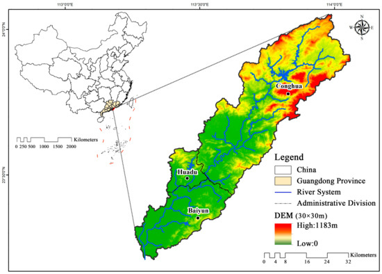
Figure 1.
The location and digital elevation map (DEM) of the Liuxihe River basin (LXH).
2.2. Data and Data Processing
Satellite images taken in 1980, 1990, 1995, 2000, 2005, 2008, 2010, and 2015 (Landsat MSS/TM/ETM, Landsat 8) with a spatial resolution of 30 m were provided by Data Center for Resources and Environmental Sciences, Chinese Academy of Sciences (http://www.resdc.cn, accessed on 30 December 2017). The method of visual interpretation was used to derive thematic land use maps based on the land resource classification system of Chinese academy of sciences [47]. Meanwhile, the accuracy of interpretation was improved through reference data, such as geomorphic maps, vegetation maps, ground truth data at different sample points, and local resident interview data. The calculated results of Kappa coefficient were larger than 0.80, which verified the accuracy and reliability of these land use maps [48]. This paper reclassified these land use maps into nine types including cropland, forest, orchard, grassland, shrub, water, floodplain, construction land, and unused land (Appendix A Table A1).
Besides, data from 1980 to 2015 about demographic factors, socioeconomic factors, and urbanized activities of the LXH were collected from the Guangzhou Statistical Yearbook (http://tjj.gz.gov.cn/, accessed on 1 April 2018) and the Outline of Guangzhou Urban Construction Overall Strategic Concept Plan (http://ghzyj.gz.gov.cn/, accessed on 30 October 2018), which is provided by the Chinese government. The detailed factors are total population (TP), proportion of non-agricultural population (PNAP), gross domestic product (GDP), proportion of primary industry (PPI), proportion of secondary industry (PSI), proportion of tertiary industry (PTI), annual per capital income (APCI), and total investment in real estate development (IRE).
Spatial data such as topographical elements (digital elevation map (DEM) and SLOPE) were obtained from NASA’s Earth Observing System Data and Information System (https://search.earthdata.nasa.gov/search, accessed on 30 December 2018). And other spatial data were obtained from Data Center for Resources and Environmental Sciences, Chinese Academy of Sciences (Source: China, Satellite images, http://www.resdc.cn, accessed on 30 December 2018), including population density (TP), socioeconomic level (GDP), urbanized activities (NLD), and land use intensity (LUIN). These main parameters of the LXH with a spatial resolution of 1000 m (except for the DEM and SLOPE data with a spatial resolution of 30 m) were all cut out by the ArcGIS software.
2.3. Methods
2.3.1. Selection of Landscape Metrics and Influencing Factors
- Landscape Metrics
The factor analysis method [49] was taken to screen the notable landscape metrics from 23 frequently used metrics (Appendix B Figure A1). First, if the absolute value of the correlation coefficient between two indices was more than 0.9, only one was used; second, indices representing different aspects of landscape characteristics were selected to reduce the information redundancy among them [50]. Five representative indices were used in the final analysis, including the patch density (PD), aggregation index (AI), largest patch index (LPI), area-weighted mean patch fractal dimension (AWMPFD), and Shannon’s diversity index (SHDI). These landscape metrics were calculated for 1980, 1990, 2000, 2010, and 2015 using the public domain software FRAGSTATS 4.2 at both the class-level and landscape-level in 14 different granularities (30 m, 50 m, 100 m, 200 m, 300 m, 400 m, 500 m, 600 m, 700 m, 800 m, 900 m, 1000 m, 1100 m, 1200 m). FRAGSTATS is a computer software program designed to compute a wide variety of landscape metrics for categorical map patterns at different levels (the detailed introduction of this software can be found at https://www.umass.edu/landeco/research/fragstats/fragstats.html, accessed on 1 February 2018). Thus, the characteristic scale interval which is appropriate for spatial analysis of the Liuxihe River basin was determined (Appendix B Figure A2). The calculation formula and ecological significance of these indices are given in Table 1.

Table 1.
Landscape metrics used in this study, their formula and ecological interpretation.
- Land Use Transition Matrix
The changes in landscapes were detected by calculating each land use type transition matrix of any two adjacent periods from 1980 to 2015. The following equation (Equation (1)) was applied to calculate the matrix:
where indicates the area in transition from landscape to . Each element of the transition matrix meets two standards: (1) is non-negative, and (2) .
For a better characterization of landscape changes, the transition matrix between any two adjacent periods was displayed in a two-dimensional table by many researchers [51]. Therein, the diagonal entries of the table reflect the total size of persistent land use types whereas the off-diagonal entries show the transition size of one land use type to another. Besides, the gross gain and gross loss of each land use type were also displayed in the table, which could be used to calculate the total exchange (sum of the gross gain and the gross loss) and net change (the gross gain minus the gross loss).
- Selection of Landscape Change Influencing Factors
The influencing factors on the development of landscape pattern vary at different spatial and temporal scales [52], which were categorized into natural and anthropogenic factors in most of the related researches [53,54]. This study focused on the small-scale watershed around rapidly urbanization city in a short research period. In these areas, anthropogenic factors such as population growth, socioeconomic activities, urbanization activities, and related policies usually play a major role [29]. In terms of natural factors, they are relatively stable and unchanged in short term compared with anthropogenic factors [55], thus their impact on landscape changes can be ignored in this case [56,57,58]. Finally, only anthropogenic factors were selected to reflect the temporal influencing factors in this study, including the total population (TP), the proportion of the non-agricultural population (PNAP), gross domestic product (GDP), the proportion of the primary industry (PPI), the proportion of the secondary industry (PSI), the proportion of the tertiary industry (PTI), annual per capita income (APCI), and total investment in real estate development (IRE). These factors are about the demographic, socioeconomic, and urbanized activities of a region. Besides these, the policies related to the rapid urbanization were also considered.
In addition, researchers found that climate conditions had no significant influence on the spatial distribution of landscape in a small-scale catchment [33], and topographical and anthropogenic factors were commonly used to interpret the landscape spatial heterogeneity in this case [28,59]. As we all know, the spatial difference of soil and hydrological conditions always depend on topographical factors. Therefore, this study mainly analyzed the spatial difference of topographical and anthropogenic factors on landscape spatial heterogeneity. Herein, the spatially distributed data of GDP and TP were selected to represent the spatial difference between socioeconomic level and population density. The nighttime light (NLD) spatial data were used to represent the urbanization degree. Moreover, the spatial distribution of the LUIN was calculated using the land use comprehensive degree index, representing the urbanization activities related to land use changes. Additional details on the calculation of land use comprehensive degree index can be found in Yu et al. [60]. Besides, the topographical variables (DEM and SLOPE) were also considered.
2.3.2. Quantifying the Influence on the Change of Landscape Pattern
Considering the spatiotemporal characteristics of land use and landscape pattern changes and their interactions, this study mainly analyzed the factors that influence the temporal change of land use types and spatial differences of landscape patterns (i.e., the spatial heterogeneity of landscape). Since the data for each year could not be obtained, it made the commonly used quantitative statistical analysis impractical. This study applied grey correlation analysis to explore the impact of different influencing factors on land use changes in an attempt to effectively solve the problem of insufficient sample data. Meanwhile, spatial correlation analysis using the Geodetector was carried out to assess the influence degree and interaction of each influencing factor toward different spatial characteristics of landscape index.
- Grey Correlation Analysis
Grey correlation analysis is an impacting factor measurement method in the grey system theory proposed by Deng [61] in 1982, which analyzes the uncertain relationship between a main factor and all other influencing factors in a given system. It can complement the defects of statistical analysis methods and can work with small amounts of irregular data; it also negates the inconsistency between quantitative and qualitative results. The analysis method mainly compares the time series of each influencing factor to determine which one is dominant. That is, when the trend of changes between an independent variable and a dependent variable is consistent or the degree of synchronization change is high, a strong correlation results [62]. The relationship is often expressed by grey correlation degree (Equation (2)). The greater the degree of grey correlation is, the more the influence degree of the factor will be and vice versa.
where and are the independent variable series and the dependent variable series, respectively; is the grey relational degree between independent variables and dependent variables ; is the resolution coefficient, , and usually takes a value of 0.5; is the time series.
- Spatial Correlation Analysis
Spatial autocorrelation can be defined as the coincidence of value similarity with location similarity, and is used to detect patterns of spatial association [63]. In this study, the global Moran’s index [64,65] (Equation (3)) was adopted to analyze the spatial autocorrelation of each landscape metric in its characteristic scale interval (500~1200 m), providing appropriate spatial scales for launching the bivariate spatial correlation analysis between each landscape metric and the influencing factors (Appendix A Table A2).
where is the spatial weight matrix between observation unit and its neighboring units : and are established by diving the study area into uniform grids based on its appropriate scale; and are the observed values of adjacent research area and , respectively; n is the number of spatial units of the research area, and is the average value of all observed values in the sample. Index ranges from −1 to 1, and as the absolute value of increases, the spatial correlation gets stronger. indicates a random spatial distribution.
Further, bivariate Moran’s [66] (Equation (4)), which is based on the principle of univariate spatial correlation, has been adopted on the specific scale of 1000 × 1000 m. On this spatial scale, the analysis scale between each landscape metric and each influencing factor can be unified. The spatial autocorrelation analysis of each landscape metric at this scale was extremely significant. Through the spatial autocorrelation analysis, the relationship between the landscape metric and spatial influencing factors was captured and the strength of the association between the two variables was measured over the study area.
where also ranges from −1 to 1, is the attribute values of adjacent research areas and , while is the attribute values of adjacent research areas and y; and are the average attribute values of x and y in the sample, respectively; and is the number of the spatial units of the research area.
- Geographical Detector Model
The geographical detector model (Geodetector), which is based on the theory of spatial stratified heterogeneity [67], was used to analyze the interaction between landscape metrics and various influencing factors in this study. First, we obtained the spatial data of independent variables through discrete classification for various influencing factors using the geometrical interval method [68,69,70], and then analyzed the influence of these variables on each landscape metric of the same spatial scales via Geodetector.
Specifically, the factor force q in Equation (5), ranging from 0 to 1, quantified the effect of different influencing factors on the spatial distribution of landscape metrics [32], and reflected the degree of spatial stratified heterogeneity of the metrics. The larger the q became, the more heterogeneous the landscape pattern.
where and stand for the number of units and the variance of the dependent variable, respectively; is the stratification of the dependent or independent variable; and stand for the number of units and the variance of the dependent variable in stratification layer , respectively.
3. Results
3.1. Spatiotemporal Variations of Land Use Types
As shown in Figure 2, the overall landscape of the LXH is dominated by forests and croplands, while other seven land use types (including forest, shrub, orchard, grassland, water, floodplain and unused land) occupy a relatively small portion, accounting for less than a quarter of the total basin. Clearly, it is noticed that the proportion change in land use types were not large in general, but their temporal and spatial differences were obvious. Therein, the proportion changes of cropland and construction land were more prominent than any other land use types, particularly in the middle and lower watershed during 2000 and 2010. Temporally, the decreases of cropland and increases of construction land in this decade were more than 50% of that in total 35 years (See subfigures b in Figure 2). Spatially, it can be seen from the results of (c) in Figure 2 that the cropland decreased by 16.96% in the lower watershed and 2.70% in the middle watershed, respectively. The construction land increased by 17.78% in the lower watershed and 3.33% in the middle watershed, respectively. Their changes were all less than 1% in the upper watershed.
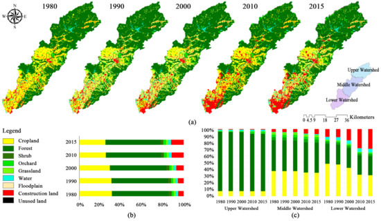
Figure 2.
The types of land use in the LXH (1980–2015) (a) Spatial distribution of land use; (b) Percent coverage of the land use types; and (c) percent coverage of the land use types in the upper, middle and lower watershed of the river basin.
More importantly, land use changes, characterized by the transition from one type to another, were extremely prominent. From the land use conversion matrix between 1980 and 2015 in Table 2, it can be calculated that the total exchange area is 578.93 km2, or 24.71% of the total catchment area. Specifically, the conversions among cropland, forest, orchard, water, and construction land comprised 94.78% of the total exchange. Among them, construction land has increased by 158.67 km2 or 127.47%. Cropland and forest have decreased by 146.33 km2 or 20.00% and 39.24 km2 or 3.08%, respectively. Other changes were all less than 20.00 km2. It can be observed that cropland and forests primarily contributed to land use exchanges and were the major land use types encroached on by urbanization. Of the 158.67 km2 increases in construction land, 89.17% resulted from conversion of cropland and 10.35% resulted from conversion of forests.
Table 2.
Land use types conversion matrix between 1980 and 2015 (km2).
Besides, there also exist great temporal and spatial differences in land use exchanges. Temporally, the Sankey diagram in Figure 3 visualizes exchanges of each land use type over different time periods. Therein, exchanges in almost all land use types during 2000–2010 are the most significant. Notably, the increase of construction land in this decade accounted for more than 50% of the total increase in the entire period, and 78.11% of the construction land increase came from conversion of cropland and 10.10% from conversion of forest. Spatially, Figure 4 shows that the conversions mainly occurred in the middle and lower reaches of the basin where a large amount of cropland was converted into construction land. Particularly, the lower reaches experienced the most drastic changes in the river basin regarding croplands and construction areas.
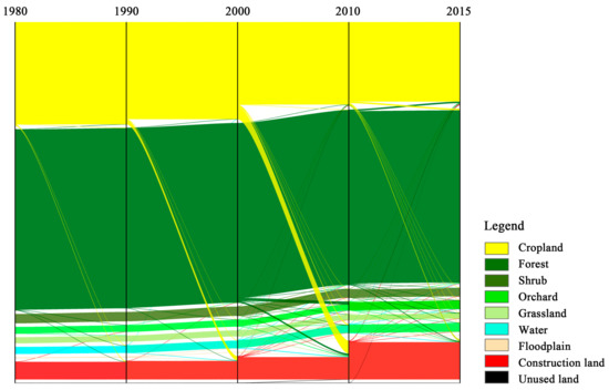
Figure 3.
Comparison of exchanges of land use types in four time periods.
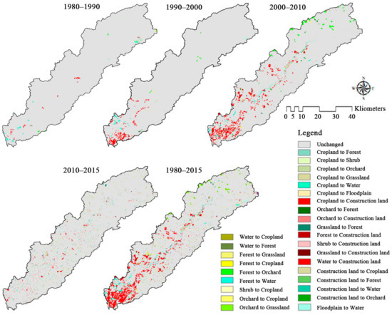
Figure 4.
Spatial variations of land use type transition in different time intervals (1980–1990, 1990–2000, 2000–2010, 2010–2015 and 1980–2015).
3.2. Spatiotemporal Variations of Landscape Patterns
The different landscape pattern indices were calculated at both landscape and land use class levels on the specific scale of 1000 × 1000 m. The former represents the overall spatial arrangement characteristics of each landscape patch, and the latter reflects the spatial arrangement characteristics of each landscape patch in different types. That is, the landscape pattern of each landscape patches at the class level can determine it at the landscape level, but not vice versa.
Figure 5 shows that changes of those indices are all obvious at the landscape level. For example, the landscape fragmentation index PD has an increasing trend and increased by 8.03%, while AI shows a decreasing trend and decreased by 2.25%. Meanwhile, the interference index AWMPFD and dominance index LPI decreased by 0.71% and 4.86%, respectively. The diversity index SHDI shows an increasing trend and increased by 5.25%. Temporally, these indices altogether indicated an increasing fragmentation and homogenization in landscapes, intensified human interference, and a weakening dominance of the once-dominant landscape (forest and cropland) in the early years. Similar to the changes in land use types, the decade from 2000–2010 experienced the most significant changes in landscape pattern.
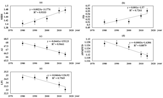
Figure 5.
Changes of landscape metrics (a) Shannon’s diversity index (SHDI), (b) patch density (PD), (c) aggregation index (AI), (d) area-weighted mean patch fractal dimension (AWMPFD), and (e) largest patch index (LPI) at the landscape level from 1980 to 2015.
Moreover, similar to land use changes, landscape pattern also showed distinct spatial characteristics, reflecting the landscape heterogeneity in the LXH. As shown in Figure 6, the PD and SHDI are relatively small while AI, AWMPFD, and LPI are relatively large in the upstream area. However, this pattern reverses in the middle and lower watershed. This indicated that the landscape in the middle and lower watershed was more fragmented and heterogeneous than the landscape in the upper watershed, with a higher interference and lower dominance. Moreover, by comparing the values of these landscape metrics in 1980 and 2015 shown in subfigures c in Figure 6, we find that they are almost unchanged in most regions, except for part of the middle and lower watershed where cropland had been largely converted to construction land.
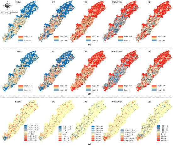
Figure 6.
Spatial distribution of the changes in landscape metrics between (a) 1980 and (b) 2015, and (c) showed the results of subtraction of the indices in 1980 from 2015.
At the land use class-level, it can be found that the PD and AI value of cropland and forest changed more significantly than the other types during the total study period. The PD of cropland and forest increased by 42.26% and 41.59%, and the AI decreased by 1.68% and 0.21%, respectively. Meanwhile, the LPI values of cropland and forest decreased by 67.45% and 3.07%, respectively. The LPI of construction land in 2015 was 12 times that of the LPI in 1980, second only to the LPI of cropland. Among all land use types, the AWMPFD of cropland decreased most significantly, by 4.39% in total, while the net change of the AWMPFD of other types was less than 1.00%. That is, the degree of fragmentation, homogenization, and human alteration of cropland in this river basin was the most significant of all terrains. At the same time, the degree of landscape dominance of cropland was greatly reduced, while that of construction land was greatly improved. This indicated that the fragmentation and homogenization of cropland was mainly contributed by occupation of the construction land.
3.3. Impacts of the Anthropogenic Factors on Temporal Landscape Changes
Since the effect of natural factors on landscape changes was minor compared with anthropogenic factors in a short period of time, this paper selected eight anthropogenic factors involving demographic factors, socioeconomic factors, and urbanized activities to reflect their impacts on landscape changes temporally (refer to Figure 7 for detailed indices and their change trends). Meanwhile, due to the difficulty of quantitatively expressing the related policies, they were not included in the following quantitative analysis.
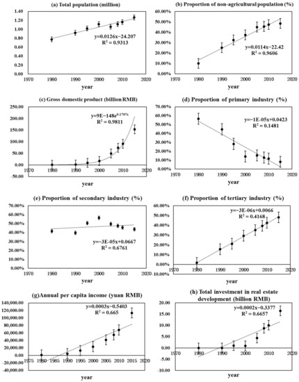
Figure 7.
Temporal trends of influencing factors (a) Total population, (b) Proportion of non-agricultural population, (c) Gross domestic product, (d) Proportion of primary industry, (e) Proportion of secondary industry, (f) Proportion of tertiary industry, (g) Annual per capita income and (h) Total investment in real estate development during 1980 to 2015.
First, from the Figure 7 and Figure 8, it can be found that the temporal changes of some influencing factors and land use types are non-linear; we chose the method of grey correlation analysis in this context. According to the results from the relational analysis in Table 3, all the grey correlation coefficients are greater than 0.55, indicating that the changes of these eight anthropogenic factors are all significantly correlated with the changes of various land use types in the LXH temporally. More specifically, the four most correlated factors on each land use type were the TP, the PNAP, the PSI, and the PTI, which were demographic and socioeconomic factors and their correlations were all above 0.73. Among them, for cropland and each natural land (forest, shrub, grassland, water, floodplain, and unused land), the most correlated factors were PSI and TP; while for construction land, the most correlated factors were PNAP and PTI. From the Figure 7, it is clear that the TP, PNAP, and PTI all increase dramatically from 1980 to 2015 in the LXH. The PSI shows a trend of first increasing and then decreasing, but it also increases on the whole. Therefore, combined with the characteristics of the proportion changes in various land use types in Figure 8, it can be concluded that the increase of construction land was mainly correlated with the increase of non-agricultural population and the continuous development of the tertiary industry in the LXH. The decreasing of cropland and each natural land was mainly correlated with the increase of TP and the changes in secondary industry. This might be attributed to the growing population (especially the growth of urban population) and the transformation of industry (especially the growth of tertiary industry), which has accelerated the encroachment on cropland and natural lands to meet the demands for more construction land in the LXH [71,72]. Alternately, the other four influencing factors were also crucial to the changes of different land use types, but they had less of an effect compared with these main influencing factors.
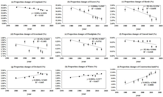
Figure 8.
Temporal trends of each land use type (a) Proportion changes of Cropland, (b) Proportion changes of Forest, (c) Proportion changes of Shrub, (d) Proportion changes of Grassland, (e) Proportion changes of Floodplain, (f) Proportion changes of Unused land, (g) Proportion changes of Orchard, (h) Proportion changes of Water and (i) Proportion changes of Construction land during 1980 to 2015.
Table 3.
Grey correlation coefficients of influencing factors on land use changes.
3.4. Impacts of Anthropogenic and Natural Factors on Spatial Landscape Changes
Considering the fact that landscape pattern experienced the most significant changes from 2000 to 2010, we took this period as an example to study the influencing factors of spatial heterogeneity toward landscape pattern in this river basin. Table 4 manifests the significant spatial correlation between each landscape metric and each investigated influencing factor in 2000 and 2010 respectively. Among them, topographic elements DEM and SLOPE were all spatially negatively correlated with PD and SHDI, and positively correlated with AI, AWMPFD, and LPI. This indicated that in areas with low elevation and gentle slopes, the degree of landscape fragmentation, landscape interference, and landscape homogenization was stronger, and that the landscape dominance was weak. Table 4 also shows that all anthropogenic influencing factors (GDP, TP, and NLD) are positively correlated with PD and SHDI, and negatively correlated with AI, AWMPFD, and LPI spatially. This illustrates that the degree of landscape fragmentation, landscape interference, and landscape homogenization is relatively strong in more developed regions. In terms of the impact of land use changes brought by rapid urbanization on landscape patterns, the LUIN was positively correlated with PD and SHDI spatially and negatively correlated with AI, AWMPFD, and LPI. This reflected that areas with high LUIN were usually accompanied with a relatively stronger degree of landscape fragmentation, landscape interference, and landscape homogenization.
Table 4.
Bivariate Moran’s I correlation analysis between landscape metrics and influencing factors in the spatial dimension in 2000 and 2010.
Geographic detector analysis showed that the interpretation of DEM on the spatial distribution of each landscape metric was the largest among all influencing factors in 2000 or 2010, with the highest average q value being 0.28 or 0.23, followed by GDP, TP, and NLD, while Slope had the lowest q value (Figure 9). Results indicated that the spatial distribution of elevation was the key factor that induced the spatial heterogeneity of landscape pattern, and the spatial distribution of socioeconomic level, population density, and urbanized activities also played an important part. The analysis of interactions between the influencing factors and landscape metrics (Figure 10) showed that the interpretation of spatial distribution characteristics of landscape pattern by any two influencing factors was greater than that of any single influencing factor, indicating that the formation of spatial heterogeneity was the result of interactions between various influencing factors. Specifically, from the subfigures a in Figure 10, the interaction between DEM and LUIN is the strongest among other factors. The interaction between LUIN and other four influencing factors on each landscape metric was almost stronger than that between any other two influencing factors in 2000. This indicated that the spatial differences of DEM and LUIN jointly resulted in the spatial heterogeneity of landscape pattern in 2000, stronger than the interactions between DEM and GDP, TP, NLD, Slope comparatively. However, compared with the results from 2000, since the interaction between DEM and TP, GDP, and NLD was strengthened, the interaction between DEM and LUIN was no longer the strongest among the other factors in 2010 (see subfigures b in Figure 10). These indicated that the spatial differences of the topographic elements and other influencing factors also jointly contributed to the spatial heterogeneity of landscape pattern in 2010.
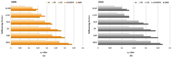
Figure 9.
The force q among each influencing factor on each landscape pattern metric in (a) 2000 and (b) 2010.
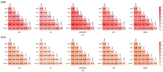
Figure 10.
The force q among any two influencing factors on each landscape pattern metric interactively in (a) 2000 and (b) 2010.
4. Discussion
4.1. Spatiotemporal Changes of Land Use and Landscape Pattern
The results of this study showed that in the LXH, there exist large spatial and temporal differences in land use changes and landscape pattern changes. These changes appeared to be more prominent in the middle and lower watershed, and their changing rates were fastest during 2000 to 2010. Specifically, the land use change was featured by the increasing transition of cropland and forest to construction land, and the fragmentation and homogenization of landscape pattern was contributed to the encroachment of construction land on forest and cropland. That is, the decrease of cropland and forest was accompanied with the decreased degree of the cropland and forest landscape dominance and the increased degree of the cropland and forest landscape fragmentation and homogenization. These further proved the synchronization characteristics and interaction relationship between land use changes and landscape pattern changes proposed by scholars [17,19]. Thus, it is possible for researchers to use the temporal change of a land use type to reflect the temporal change pattern of a certain landscape type in a period of time.
Besides, our findings of the land use and landscape pattern changes are consistent with the previous research in the whole Guangzhou city. For example, Zhang et al. [73] and Gong et al. [74] also found that the increase of construction land in new urban areas of Guangzhou city mainly came from cropland, forest, and other ecological land, especially after 2000. Gong et al. [41] also confirmed that the fragmentation and homogenization of cropland in Guangzhou was mainly contributed by the expansion of construction land. However, their research paid more attention to the urbanization expansion pattern of Guangzhou by comparing the changing differences of certain land use types and landscape patterns in different jurisdictions, instead of focusing on these spatiotemporal changes brought by urbanization [38,75]. Researches on the analysis of land use and landscape pattern changes in a watershed under the urbanization expansion pattern also exist, which provide theoretical basis and method reference for this study. But watersheds selected in their studies are relatively large, spanning multiple cities [9,21]. As a case study in this paper, the LXH was relatively small and in the range of Guangzhou city. Its middle and lower watershed is adjacent to the central urban area of Guangzhou, while the upstream area is far away from the central urban. This pushed the gradual widening of the difference between the northern and southern parts of the watershed influenced by urbanization. Our results also found that changes of land use and landscape pattern were different between the northern and southern parts.
Moreover, analysis results above reflected that the time period from 2000 to 2010 and the southern parts of the LXH with the most prominent changes should be taken seriously by relevant stakeholders. First, changes of land use and landscape pattern in southern parts of the LXH should be slow down and controlled, and the northern parts should be protected timely under the rapidly urbanizing trends. Then, the special time period from 2000 to 2010 needs to pay much attention to in related researches about the LXH. It means that this study gives not only a supplement to previous studies in these regions, but also is of great value for managers, planners, and scholars to make appropriate strategies.
4.2. The Temporal and Spatial Influencing Factors
In terms of the influencing factors of the changes of land use types and landscape patterns, previous studies mainly discussed the reasons for land use type conversion at different locations [32,76] and in different time periods [21,29], but few analyzed the factors responsible for the spatial heterogeneity of landscape patterns in river basins, nor did they comprehensively quantify the factors that contributed to the spatiotemporal change of land use types and landscape patterns. In this study, considering the fact that various land use type changes emphasized the transition of different landscape patches in different time periods, and that changes of landscape patterns reflected the difference of spatial configuration characteristics in different landscape patches, we analyzed the influencing factors on the temporal change of land use types and spatial heterogeneity of landscape pattern, respectively. We found that there was a greater difference in the spatiotemporal influencing factors of land use and landscape pattern changes in the LXH. Thus, it is very important to propose a targeted protection and development strategy, which can meet the current needs of the different regions in the LXH. Temporally, we found that the demographic factors, socioeconomic factors, and urbanized activities were important in shaping the temporal variations of land use types in this river basin, and changes of major land use types were more sensitive to the increasing of non-agricultural population and transformation of industry than any other factors. This was consistent with the findings in other studies on the influencing factors of land use types changes in other river basins [15,28]; they also found that the growth of urban population and changes of industries contributed to the increase of construction land [4,77]. Moreover, similar studies elsewhere underlined that government policy also played an important role in the change of land use types during different periods [78,79,80]. Although there was no appropriate method for analyzing the impact of the related policies on land use changes quantitatively, we found that various land use types in the LXH have undergone significant changes in the last three decades after 1980, and these changes were particularly dramatic after 2000. Zhang et al. [73] found that the implementation of China’s reform and development policy in 1978 was an important driving force for economic development and population migration of Guangzhou, pushing the continuous expansion of construction land to gradually occupy the cropland, forest, shrub, and grassland in the suburbs. Thus, the observed expansion of the construction land in the LXH after the early 1980s may be attributed to the implementation of this policy. In addition, the overall urban development master plan of Guangzhou in 2000 had put forward the strategy of expanding the urban area to the north and built Guangzhou into an international metropolis by 2010, which could further accelerate the expansion of construction land if practices continue. Correspondingly, the land use types in the LXH changed significantly after 2000 compared with the pre-2000 practices, accounting for more than 50% of the total variation in 35 years. Moreover, Baiyun, Huadu, and Conghua districts in the north had successively merged into the jurisdiction of Guangzhou in the year 2000, 2010, and 2015, respectively. The different speed of urbanization in different regions altered the variation characteristics of land use types. We also found that the lower watershed that contains the Baiyun and Huadu districts had the largest proportion of cropland conversion to construction land, which was five times higher than that of the upper and middle watershed. Therefore, apart from the demographic factors, socioeconomic factors, and urbanized activities, the relevant government policy, which is difficult to quantify, also significantly affected the variations of land use types.
Focusing on the impact of various influencing factors on landscape pattern changes in spatial dimension will be very useful in identifying and controlling the major driving forces, guiding the watershed protective management and sustainable planning. However, most of the current studies adopted the classification method to describe the spatial characteristics of landscape pattern and their influencing factors of different regions, and seldom analyzed the spatial relationships among variables quantitatively [9,33]. In the research of Ju et al. [70], the applicability of the geographic detector model in analyzing the driving force of construction land expansion was proved, providing a quantitative method for the analysis of the interaction among various spatial factors. But their research did not conduct a comparative analysis of the spatial driving relationships in different periods. Here, using the model of geographic detector by Wang et al. [69], this study compared the impact of different influencing factors on spatial landscape heterogeneity during 2000 and 2010, when the most dramatic land use changes happened. It can be found that the spatial distribution of LUIN and elevation were the two critical factors for the formation of landscape heterogeneity in 2000 compared with other factors, while the interaction between elevation and other human factors was strengthened in 2010; this illustrated that elevation was always a basic factor that directly determined the spatial distribution of landscape pattern. Liu et al. [61] also proposed that it was difficult for people to break through existing natural obstacles in the hilly regions of southern China, and this difficulty had largely restricted human activities. From Figure 11, it is clear that great differences in the terrain conditions exist in this study. Because areas with high elevation or greater slopes were difficult to develop and not suitable for urban construction, they were seldom disturbed by human activities [33], so that the degree of landscape fragmentation and homogenization in the upper reaches was low and the degree of landscape dominance was high. Therefore, elevation was a prerequisite for the impact of anthropogenic factors to occur. On the other hand, based on the difference of elevation in different regions of LXH, the human influencing factors, such as population and socioeconomic and urbanized activities, played an increasing role in the formation of the heterogeneous characteristics of the landscape pattern after 2000. This may be due to the fact that the spatial difference of human influence factors increased significantly after 2000, as it shown in subfigure c in Figure 11.
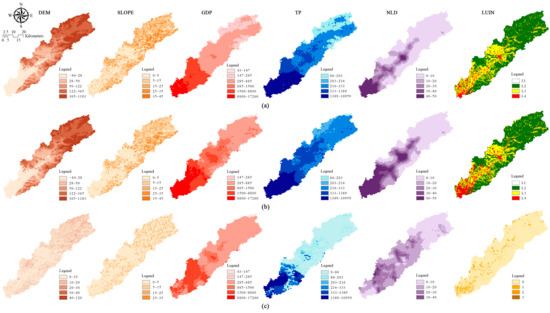
Figure 11.
Spatial distributions of the selected influencing factors selected in this study in (a) 2000 and (b) 2010, and (c) shows the results of the subtraction of each influencing factor between 2000 and 2010.
The above discussion illustrates that it is necessary to control the increasing trends of non-agricultural population and the continuous development of secondary and tertiary industry in the future, thus the demand for more construction land will be decreased. Meanwhile, relevant policies should try to meet these demands. We also should pay much attention to the southern parts of the LXH, and strengthen its adjustment ability to deal with the intensive population density, higher GDP, and greater urban construction. For example, the urban occupancy rate in these areas can be increased, artificial green land can be increased, the native forest and grassland must be strictly protected, etc. This means that establishing the spatiotemporal change trends and causes of land use and landscape pattern in a rapidly urbanizing watershed is very important for guiding the diagnosing of urbanization problems, clarifying the main protection areas and main control factors.
4.3. The Limitations and Potential Outlooks
This study produces a quantitative estimate of the spatiotemporal variations in land use types and landscape patterns and analyzes the dominant influencing factors leading to these changes in LXH quantitatively, which provides a systematic integration and deepening of previous studies. The main land use maps used in this study interpreted by the common method of visual interpretation, and their errors mainly came from the personal subjective judgment of the interpreters and the similarity of the tones and textures of the satellite image. Although these errors in the interpretation process were considered and improved through some reference maps (including topographic maps, vegetation maps, ground truth data at different sample points, and local resident interview data), there also existed uncertainties in the data measurement and description [36]. These errors will also affect the accuracy of the research results to some degree. Therefore, it is necessary to compare any two measurement methods to improve the analysis accuracy of land use maps and express them on different scales as much as possible in the future. Besides, due to the scarcity of historical landscape information, e.g., land use maps from 1980 to 2015, Topography data and Nighttime Light Image Data in 2015, we were unable to accurately establish the relationship between each land use type and different influencing factors, nor could we compare the driving factors of spatial heterogeneity of landscape patterns in each period. In addition, there are some factors that cannot be quantified, such as policy factors, which make the analysis of influencing factors still not comprehensive enough. In the future, it may be possible to construct a comprehensive model combining qualitative and quantitative analysis on all possible influencing factors of land use changes.
Resolution of available spatial data set of spatial influencing factors was also a limitation. We conducted the driving analysis between the influencing factors and landscape indices at a 1 km grid. Although on this scale the influencing factors also had good spatial correlation, the resolution limitation of influencing factors might affect the accuracy of the analysis results to some degree. Therefore, spatial data with appropriate accuracy at a higher resolution and longer periods could substantially improve the accuracy when analyzing the change of landscape patterns and their driving forces. In that sense, models of land use change would be a good alternative for such studies by simulating the land use in different years to increase the range and length of land use data [81], and hence guide the urbanization development of this region by analyzing the change of land use types and landscape patterns in the future. Moreover, the extensive establishment of the real-time monitoring data platform of different spatial influencing factors such as social economic activities, population density, and urbanization activities in the future with higher resolution will improve the accuracy of spatial analysis, thereby realizing its dynamic analysis.
Moreover, based on our comprehensive analysis of the spatiotemporal changes and causes of landscape pattern in the LXH and its ecological and hydrological effects in related researches [43], it is more urgent to establish specific strategies to guide the sustainable development of LXH in the future. The Hellwig classification and measurement method introduced by Hellwig in 1968 provides a decision-making method for formulating sustainable development strategies based on the evaluating of urban development [82]. This method was first applied in the sustainable decision-making process of urban green space biodiversity management in Lublin, eastern of Poland, thus the main ecological areas that should be protected can be established [83]. Then, other scholars used and extended this method at different scales in European Union to formulate sustainable development strategies based on the different goals. These application of the Hellwig method in different researches prove its effectiveness in evaluating the level of development of different regions in different fields at different scales, which provide a new direction for the future research of establishing the sustainable development strategy in the LXH based on the analysis of its changes about land use, landscape pattern, hydrological and ecological conditions under the rapid urbanization. After that, the specific areas of the LXH under the rapid urbanization process, in which its land use transition and landscape pattern fragmentation should be extremely controlled can be found.
5. Conclusions
In this study, we analyzed the spatiotemporal changes of land use types and landscape pattern of the LXH from 1980 to 2015 under the rapid urbanization of Guangzhou city, as well as quantified the major influencing factors temporally and spatially. The main conclusion can be concluded as one sentence that there exist great spatiotemporal differences in land use and landscape pattern changes and its causes in the LXH during the past 35 years. Specifically, it can be drawn as follows:
- The most obvious land use change was characterized as the large transition from cropland to construction land, bringing about the fragmentation of cropland that was encroached on by the construction land. The landscape pattern showed an increasing trend of landscape fragmentation, homogenization, and landscape interference, and a decreasing trend in landscape dominance. These changes mainly occurred in the lower watershed, particularly between 2000 and 2010. Therein, these changes were more than 50% in this decade compared with total 35 years.
- Many influencing factors affected the temporal variations in landscapes, including population growth, economic and industrial development, urbanized activities, and relevant policies. Among them, changes of major land use types were more sensitive to the increase of a non-agricultural population and transformation of industries than other factors. In addition, the spatial distribution of land use types and elevation were found to be the two key factors for the formation of landscape heterogeneity in 2000, while the spatial distribution of the other three human factors and elevation gradually became the same important factors after 2000.
- Our research shows that the temporal and spatial difference of changes in land use and landscape pattern at a watershed with unbalance urbanization degree in different regions was great. This is not only affected by the difference of the degree in socioeconomic level, population growth rate, and urbanizing expansion in different time and space, but also determined by the related policies. Besides, the topographical factors were also the basis of the formation on landscape pattern. When developing, we need to consider both the geographical conditions and the urbanizing degree of the watershed, thus a sustainable development strategy could be formulated and the goals of protecting and restoring the watershed ecosystem can be achieved.
The findings are of great significance for review and outlook of the ecological protection and sustainable development of the watershed around the rapidly urbanizing areas. It can not only allow decision-makers to clarify their main problems, but also guide them to clarify the key protection areas and control indicators. However, the analysis of the landscape patterns above was limited to the period from 1980 to 2015, and the comparison of influencing factors on spatial landscape configurations focused only on 2000 and 2010. Nonetheless, results in this study are insightful, although they could be more generalized with the analysis over a longer period.
Author Contributions
Conceptualization, Z.Z. and B.L.; methodology, Z.Z.; software, Z.Z.; validation, Z.Z., H.W., and M.H.; formal analysis, Z.Z. H.W., and M.H.; investigation, Z.Z. and B.L.; resources, B.L.; data curation, B.L.; writing—original draft preparation, Z.Z.; writing—review and editing, Z.Z., B.L., H.W., and M.H.; visualization, Z.Z.; supervision, B.L.; project administration, B.L.; funding acquisition, B.L. All authors have read and agreed to the published version of the manuscript.
Funding
This research was funded by the National Natural Science Foundation of China (Grant Nos. 51879289), the Guangdong Basic and Applied Basic Research Foundation (2019B1515120052) and the Innovation Fund of Guangzhou City water science and technology (GZSWKJ-2020-2).
Institutional Review Board Statement
Not applicable.
Informed Consent Statement
Not applicable.
Data Availability Statement
The data presented in this study are available on request from the corresponding website.
Acknowledgments
We would like to thank the editor Madalina Buzatu and three anonymous reviewers for their constructive comments.
Conflicts of Interest
The authors declare no conflict of interest.
Appendix A
Table A1.
Description of land use types in the LXH.
Table A1.
Description of land use types in the LXH.
| Land Use Types | Description |
|---|---|
| Cropland | Arable agricultural land, including paddy fields and dry land |
| Forest | Natural and semi-natural manmade woodland |
| Shrub | Dwarf woodland (height < 2 m) and shrubbery |
| Orchard | Intensively managed orchards (fruit orchards, mulberry orchards, tea orchards) and plant nursery |
| Grassland | Natural and artificial grassland |
| Water | Rivers, creeks, canals, ponds, lakes, reservoirs, and bays |
| Floodplain | Permanent and seasonal floodplains |
| Construction land | Mainly urban and rural settlements, mining land, transportation land, and other special construction land |
| Unused land | Mainly land without vegetation cover and difficult to use, including bare soil, sandy land, desert, saline, and landfills |
Table A1 gives a detailed description of the content about each land use type in this study, which can better display the classification standard of land use types.
Table A2.
Analysis results of spatial autocorrelation of each landscape metric in different scales in 2000 and 2015 of LXH
Table A2.
Analysis results of spatial autocorrelation of each landscape metric in different scales in 2000 and 2015 of LXH
| Scales/(m × m) | PD | AI | AWMPFD | LPI | SHDI | |||||
|---|---|---|---|---|---|---|---|---|---|---|
| 2000 | 2015 | 2000 | 2015 | 2000 | 2015 | 2000 | 2015 | 2000 | 2015 | |
| 500 × 500 m | 0.47 | 0.47 | 0.45 | 0.45 | 0.46 | 0.47 | 0.47 | 0.46 | 0.47 | 0.47 |
| 600 × 600 m | 0.47 | 0.47 | 0.45 | 0.45 | 0.46 | 0.47 | 0.47 | 0.46 | 0.47 | 0.47 |
| 700 × 700 m | 0.46 | 0.46 | 0.45 | 0.45 | 0.46 | 0.46 | 0.46 | 0.46 | 0.46 | 0.46 |
| 800 × 800 m | 0.46 | 0.46 | 0.43 | 0.43 | 0.45 | 0.46 | 0.46 | 0.45 | 0.46 | 0.46 |
| 900 × 900 m | 0.46 | 0.46 | 0.43 | 0.43 | 0.45 | 0.46 | 0.46 | 0.45 | 0.46 | 0.46 |
| 1000 × 1000 m | 0.44 | 0.44 | 0.42 | 0.42 | 0.43 | 0.44 | 0.44 | 0.43 | 0.44 | 0.44 |
| 1100 × 1100 m | 0.44 | 0.44 | 0.41 | 0.41 | 0.43 | 0.44 | 0.44 | 0.43 | 0.44 | 0.44 |
| 1200 × 1200 m | 0.44 | 0.44 | 0.44 | 0.44 | 0.44 | 0.44 | 0.44 | 0.44 | 0.44 | 0.44 |
Note: Permutation test was used to test in this study, and the P value of each landscape metrics in different scales was equal to 0, indicating that the spatial correlation was significant under 99.9% confidence. The Z value of them were all >1.96, reflecting that there exists extremely significant spatial autocorrelation among these landscape metrics in different spatial scales.
Table A2 reflects the degree of spatial autocorrelation about each landscape metric selected in this paper. It confirms that the spatial autocorrelation of these landscape metrics is extremely significant in different spatial scales ranging from 500 to 1200 m. Therefore, it can be proved that these spatial scales are all appropriate for analyzing the bivariate spatial correlation between each landscape metric and each influencing factor.
Appendix B
This Figure A1 is provided to screen the notable landscape metrics from 23 frequently used metrics. It demonstrates the correlation between any two kinds of landscape metrics among these 23 metrics above. Clearly, most of them were highly correlated with each other. Thus, when the absolute value of correlation coefficient between two indices is more than 0.9, only one is used; second, indices representing different aspects of landscape characteristics were selected to reduce the information redundancy among them. Finally, five representative indices were selected in this paper, including patch density (PD), aggregation index (AI), largest patch index (LPI), area-weighted mean patch fractal dimension (AWMPFD), and Shannon’s diversity index (SHDI), which represent different aspects of landscape characteristics.

Figure A1.
Results of the factor analysis among 23 common metrics.
Figure A1.
Results of the factor analysis among 23 common metrics.

Figure A2 presents the changing value of five selected landscape metrics at landscape-level in 14 different granularities (including 30 m, 50 m, 100 m, 200 m, 300 m, 400 m, 500 m, 600 m, 700 m, 800 m, 900 m, 1000 m, 1100 m, 1200 m). It proves that 500~1200 m was the common characteristics interval of these landscape metrics. Thus, the spatial scale for analyzing the spatial autocorrelation of each landscape metric has been established.

Figure A2.
Analysis results of the characteristic scale interval in 14 different granularities.
Figure A2.
Analysis results of the characteristic scale interval in 14 different granularities.

References
- Deng, J.S.; Wang, K.; Hong, Y.; Qi, J.G. Spatio-temporal dynamics and evolution of land use change and landscape pattern in response to rapid urbanization. Landsc. Urban Plan. 2009, 92, 187–198. [Google Scholar] [CrossRef]
- Sui, D.Z.; Zeng, H. Modeling the dynamics of landscape structure in Asia’s emerging desakota regions: A case study in Shenzhen. Landsc. Urban Plan. 2002, 53, 37–52. [Google Scholar] [CrossRef]
- Liu, Y.; Yao, C.; Wang, G.; Bao, S. An integrated sustainable development approach to modeling the eco-environmental effects from urbanization. Ecol. Indic. 2011, 11, 1599–1608. [Google Scholar] [CrossRef]
- Liu, Y.; Luo, T.; Liu, Z.; Kong, X.; Li, J.; Tan, R. A comparative analysis of urban and rural construction land use change and driving forces: Implications for urban-rural coordination development in Wuhan, Central China. Habitat Int. 2015, 47, 113–125. [Google Scholar] [CrossRef]
- Meyfroidt, P.; Lambin, E.F.; Erb, K.H.; Hertel, T.W. Globalization of land use: Distant drivers of land change and geographic displacement of land use. Curr. Opin. Environ. Sustain. 2013, 5, 438–444. [Google Scholar] [CrossRef]
- Luo, P.; Mu, D.; Xue, H.; Ngo-Duc, T.; Dang-Dinh, K.; Takara, K.; Nover, D.; Schladow, G. Flood inundation assessment for the Hanoi Central Area, Vietnam under historical and extreme rainfall conditions. Sci. Rep. 2018, 8, 12623. [Google Scholar] [CrossRef]
- Zhu, Y.; Luo, P.; Zhang, S.; Sun, B. Spatiotemporal analysis of hydrological variations and their impacts on vegetation in semiarid areas from multiple satellite data. Remote Sens. 2020, 12, 4177. [Google Scholar] [CrossRef]
- Edge, C.B.; Fortin, M.J.; Jackson, D.A.; Lawrie, D.; Stanfield, L.; Shrestha, N. Habitat alteration and habitat fragmentation differentially affect beta diversity of stream fish communities. Landsc. Ecol. 2017, 32, 647–662. [Google Scholar] [CrossRef]
- Tang, J.; Li, Y.; Cui, S.; Xu, L.; Ding, S.; Nie, W. Linking land-use change, landscape patterns, and ecosystem services in a coastal watershed of southeastern China. Glob. Ecol. Conserv. 2020, 23, e01177. [Google Scholar] [CrossRef]
- Xiao, J.; Shen, Y.; Ge, J.; Tateishi, R.; Tang, C.; Liang, Y.; Huang, Z. Evaluating urban expansion and land use change in Shijiazhuang, China, by using GIS and remote sensing. Landsc. Urban Plan. 2006, 75, 69–80. [Google Scholar] [CrossRef]
- Li, X.; Yeh, A.G. Analyzing spatial restructuring of land use patterns in a fast growing region using remote sensing and GIS. Landsc. Urban Plan. 2004, 69, 335–354. [Google Scholar] [CrossRef]
- Li, C.; Zhang, Y.; Kharel, G.; Zou, C.B. Impact of Climate Variability and Landscape Patterns on Water Budget and Nutrient Loads in a Peri-urban Watershed: A Coupled Analysis Using Process-based Hydrological Model and Landscape Indices. Environ. Manag. 2018, 61, 954–967. [Google Scholar] [CrossRef]
- Liu, J.; Shen, Z.; Chen, L. Assessing how spatial variations of land use pattern affect water quality across a typical urbanized watershed in Beijing, China. Landsc. Urban Plan. 2018. [Google Scholar] [CrossRef]
- Shen, Z.; Hou, X.; Li, W.; Aini, G.; Chen, L.; Gong, Y. Impact of landscape pattern at multiple spatial scales on water quality: A case study in a typical urbanised watershed in China. Ecol. Indic. 2015. [Google Scholar] [CrossRef]
- Zhao, R.; Chen, Y.; Shi, P.; Zhang, L.; Pan, J.; Zhao, H. Land use and land cover change and driving mechanism in the arid inland river basin: A case study of Tarim River, Xinjiang, China. Environ. Earth Sci. 2013, 68, 591–604. [Google Scholar] [CrossRef]
- Mallinis, G.; Koutsias, N.; Arianoutsou, M. Monitoring land use/land cover transformations from 1945 to 2007 in two peri-urban mountainous areas of Athens metropolitan area, Greece. Sci. Total Environ. 2014, 490, 262–278. [Google Scholar] [CrossRef]
- Křováková, K.; Semerádová, S.; Mudrochová, M.; Skaloš, J. Landscape functions and their change—A review on methodological approaches. Ecol. Eng. 2015, 75, 378–383. [Google Scholar] [CrossRef]
- Forman, R.T.T. Some general principles of landscape and regional ecology. Landsc. Ecol. 1995. [Google Scholar] [CrossRef]
- Li, X.; Lu, L.; Cheng, G.; Xiao, H. Quantifying landscape structure of the Heihe River Basin, north-west China using FRAGSTATS. J. Arid Environ. 2001. [Google Scholar] [CrossRef]
- Teixeira, Z.; Teixeira, H.; Marques, J.C. Systematic processes of land use/land cover change to identify relevant driving forces: Implications on water quality. Sci. Total Environ. 2014, 470–471, 1320–1335. [Google Scholar] [CrossRef]
- Gao, C.; Zhou, P.; Jia, P.; Liu, Z.; Wei, L.; Tian, H. Spatial driving forces of dominant land use/land cover transformations in the Dongjiang River watershed, Southern China. Environ. Monit. Assess. 2016, 188. [Google Scholar] [CrossRef]
- Dadashpoor, H.; Azizi, P.; Moghadasi, M. Land use change, urbanization, and change in landscape pattern in a metropolitan area. Sci. Total Environ. 2019, 655, 707–719. [Google Scholar] [CrossRef]
- Pan, D.; Domon, G.; Marceau, D.; Bouchard, A. Spatial pattern of coniferous and deciduous forest patches in an Eastern North America agricultural landscape: The influence of land use and physical attributes. Landsc. Ecol. 2001. [Google Scholar] [CrossRef]
- Song, X.P.; Hansen, M.C.; Stehman, S.V.; Potapov, P.V.; Tyukavina, A.; Vermote, E.F.; Townshend, J.R. Global land change from 1982 to 2016. Nature 2018. [Google Scholar] [CrossRef]
- Da Silva, A.M.; Huang, C.H.; Francesconi, W.; Saintil, T.; Villegas, J. Using landscape metrics to analyze micro-scale soil erosion processes. Ecol. Indic. 2015, 56, 184–193. [Google Scholar] [CrossRef]
- Su, S.; Hu, Y.; Luo, F.; Mai, G.; Wang, Y. Farmland fragmentation due to anthropogenic activity in rapidly developing region. Agric. Syst. 2014, 131, 87–93. [Google Scholar] [CrossRef]
- Zhang, W.; Yu, N.; Liu, M.; Hu, Y.M. Landscape pattern and driving forces in the upper reaches of Minjiang River, China. In Proceedings of the 2010 3rd International Congress on Image and Signal Processing, Yantai, China, 16–18 October 2010; Volume 5, pp. 2189–2193. [Google Scholar] [CrossRef]
- Shi, Y.; Xiao, J.; Shen, Y.; Yamaguchi, Y. Quantifying the spatial differences of landscape change in the Hai River Basin, China, in the 1990s. Int. J. Remote Sens. 2012, 33, 4482–4501. [Google Scholar] [CrossRef]
- Su, S.; Wang, Y.; Luo, F.; Mai, G.; Pu, J. Peri-urban vegetated landscape pattern changes in relation to socioeconomic development. Ecol. Indic. 2014, 46, 477–486. [Google Scholar] [CrossRef]
- Zhang, F.; Kung, H.T.; Johnson, V.C. Assessment of land-cover/land-use change and landscape patterns in the two national nature reserves of Ebinur Lake Watershed, Xinjiang, China. Sustainability 2017, 9, 724. [Google Scholar] [CrossRef]
- Liu, S.; Yu, Q.; Wei, C. Spatial-Temporal Dynamic Analysis of Land Use and Landscape Pattern in Guangzhou, China: Exploring the Driving Forces from an Urban Sustainability Perspective. Sustainability 2019, 11, 6675. [Google Scholar] [CrossRef]
- Gong, Y.; Li, J.; Li, Y. Spatiotemporal characteristics and driving mechanisms of arable land in the Beijing-Tianjin-Hebei region during 1990–2015. Socioecon. Plann. Sci. 2019. [Google Scholar] [CrossRef]
- Wang, L.J.; Wu, L.; Hou, X.Y.; Zheng, B.H.; Li, H.; Norra, S. Role of reservoir construction in regional land use change in Pengxi River basin upstream of the Three Gorges Reservoir in China. Environ. Earth Sci. 2016, 75. [Google Scholar] [CrossRef]
- López-Barrera, F.; Manson, R.H.; Landgrave, R. Identifying deforestation attractors and patterns of fragmentation for seasonally dry tropical forest in central Veracruz, Mexico. Land Use Policy 2014, 41, 274–283. [Google Scholar] [CrossRef]
- McSherry, L.; Steiner, F.; Ozkeresteci, I.; Panickera, S. From knowledge to action: Lessons and planning strategies from studies of the upper San Pedro basin. Landsc. Urban Plan. 2006, 74, 81–101. [Google Scholar] [CrossRef]
- Piovan, S.E. Remote Sensing. In The Geohistorical Approach; Springer Geography; Springer: Cham, Switzerland, 2020; pp. 171–197. [Google Scholar] [CrossRef]
- Southworth, J.; Nagendra, H.; Tucker, C. Fragmentation of a landscape: Incorporating landscape metrics into satellite analyses of land-cover change. Landsc. Res. 2002. [Google Scholar] [CrossRef]
- Yu, X.; Ng, C. An integrated evaluation of landscape change using remote sensing and landscape metrics: A case study of Panyu, Guangzhou. Int. J. Remote Sens. 2006. [Google Scholar] [CrossRef]
- He, Y.; Wang, W.; Chen, Y.; Yan, H. Assessing spatio-temporal patterns and driving force of ecosystem service value in the main urban area of Guangzhou. Sci. Rep. 2021. [Google Scholar] [CrossRef]
- Guo, L.; Xia, B.; Liu, W.; Jiang, X. Spatio-temporal change and gradient differentiation of landscape pattern in Guangzhou City during its urbanization. Chin. J. Appl. Ecol. 2006, 17, 1671–1676. [Google Scholar]
- Gong, J.; Hu, Z.; Chen, W.; Liu, Y.; Wang, J. Urban expansion dynamics and modes in metropolitan Guangzhou, China. Land Use Policy 2018. [Google Scholar] [CrossRef]
- Zhang, Y.; Wang, T.; Cai, C.; Li, C.; Liu, Y.; Bao, Y.; Guan, W. Landscape pattern and transition under natural and anthropogenic disturbance in an arid region of northwestern China. Int. J. Appl. Earth Obs. Geoinf. 2016, 44, 1–10. [Google Scholar] [CrossRef]
- Zhao, P.; Xia, B.; Hu, Y.; Yang, Y. A spatial multi-criteria planning scheme for evaluating riparian buffer restoration priorities. Ecol. Eng. 2013, 54, 155–164. [Google Scholar] [CrossRef]
- Li, Q.; Xu, X.L.; Huang, J.R. Length-weight relationships of 16 fish species from the Liuxihe national aquatic germplasm resources conservation area, Guangdong, China. J. Appl. Ichthyol. 2014, 30, 434–435. [Google Scholar] [CrossRef]
- Zhang, C.; Xia, B.; Lin, J. A basin-scale estimation of carbon stocks of a forest ecosystem characterized by spatial distribution and contributive features in the Liuxihe River basin of pearl river delta. Forests 2016, 7, 299. [Google Scholar] [CrossRef]
- Yu, X.J.; Ng, C.N. Spatial and temporal dynamics of urban sprawl along two urban-rural transects: A case study of Guangzhou, China. Landsc. Urban. Plan. 2007, 79, 96–109. [Google Scholar] [CrossRef]
- Jiyuan, L.; Mingliang, L.; Xiangzheng, D.; Dafang, Z.; Zengxiang, Z.; Di, L. The land use and land cover change database and its relative studies in China. J. Geogr. Sci. 2002, 12, 275–282. [Google Scholar] [CrossRef]
- Liu, J.; Liu, M.; Tian, H.; Zhuang, D.; Zhang, Z.; Zhang, W.; Tang, X.; Deng, X. Spatial and temporal patterns of China’s cropland during 1990–2000: An analysis based on Landsat TM data. Remote Sens. Environ. 2005, 98, 442–456. [Google Scholar] [CrossRef]
- Riitters, K.H.; O’Neill, R.V.; Hunsaker, C.T.; Wickham, J.D.; Yankee, D.H.; Timmins, S.P.; Jones, K.B.; Jackson, B.L. A factor analysis of landscape pattern and structure metrics. Landsc. Ecol. 1995. [Google Scholar] [CrossRef]
- Cushman, S.A.; McGarigal, K.; Neel, M.C. Parsimony in landscape metrics: Strength, universality, and consistency. Ecol. Indic. 2008, 8, 691–703. [Google Scholar] [CrossRef]
- Pontius, R.G.; Shusas, E.; McEachern, M. Detecting important categorical land changes while accounting for persistence. Agric. Ecosyst. Environ. 2004. [Google Scholar] [CrossRef]
- Schneeberger, N.; Bürgi, M.; Hersperger, A.M.; Ewald, K.C. Driving forces and rates of landscape change as a promising combination for landscape change research-An application on the northern fringe of the Swiss Alps. Land Use Policy 2007. [Google Scholar] [CrossRef]
- Su, C.; Fu, B.; Lu, Y.; Lu, N.; Zeng, Y.; He, A.; Halina, L. Land use change and anthropogenic driving forces: A case study in Yanhe River Basin. Chin. Geogr. Sci. 2011, 21, 587–599. [Google Scholar] [CrossRef]
- Kavian, A.; Jafarian Jeloudar, Z. Land use/cover change and driving force analyses in parts of northern Iran using RS and GIS techniques. Arab. J. Geosci. 2011, 4, 401–411. [Google Scholar] [CrossRef]
- Fang, G.; Zhang, Y.; Yang, J. Evolution of urban landscape pattern in Suzhou City during 1987–2009. Appl. Mech. Mater. 2012, 178–181, 332–336. [Google Scholar] [CrossRef]
- Wang, Z.; Zhang, Y.; Zhang, B.; Song, K.; Guo, Z.; Liu, D.; Li, F. Landscape dynamics and driving factors in Da’an County of Jilin Province in Northeast China During 1956–2000. Chin. Geogr. Sci. 2008. [Google Scholar] [CrossRef]
- Bürgi, M.; Straub, A.; Gimmi, U.; Salzmann, D. The recent landscape history of Limpach valley, Switzerland: Considering three empirical hypotheses on driving forces of landscape change. Landsc. Ecol. 2010, 25, 287–297. [Google Scholar] [CrossRef]
- Hersperger, A.M.; Bürgi, M. Going beyond landscape change description: Quantifying the importance of driving forces of landscape change in a Central Europe case study. Land Use Policy 2009, 26, 640–648. [Google Scholar] [CrossRef]
- Liu, X.; Li, Y.; Shen, J.; Fu, X.; Xiao, R.; Wu, J. Landscape pattern changes at a catchment scale: A case study in the upper Jinjing river catchment in subtropical central China from 1933 to 2005. Landsc. Ecol. Eng. 2014, 10, 263–276. [Google Scholar] [CrossRef]
- Yu, G.; Li, M.; Tu, Z.; Yu, Q.; Jie, Y.; Xu, L.; Dang, Y.; Chen, X. Conjugated evolution of regional social-ecological system driven by land use and land cover change. Ecol. Indic. 2018, 89, 213–226. [Google Scholar] [CrossRef]
- Ju-Long, D. Control problems of grey systems. Syst. Control. Lett. 1982. [Google Scholar] [CrossRef]
- Chen, M.; Lu, Y.; Ling, L.; Wan, Y.; Luo, Z.; Huang, H. Drivers of changes in ecosystem service values in Ganjiang upstream watershed. Land Use Policy 2015, 47, 247–252. [Google Scholar] [CrossRef]
- Tobler, W.R. A Computer Movie Simulating Urban Growth in the Detroit Region. Econ. Geogr. 1970. [Google Scholar] [CrossRef]
- Moran, P.A. Notes on continuous stochastic phenomena. Biometrika 1950. [Google Scholar] [CrossRef]
- Cui, C.; Wang, J.; Wu, Z.; Ni, J.; Qian, T. The socio-spatial distribution of leisure venues: A case study of karaoke bars in Nanjing, China. ISPRS Int. J. Geo-Inf. 2016, 5, 150. [Google Scholar] [CrossRef]
- Wartenberg, D. Multivariate Spatial Correlation: A Method for Exploratory Geographical Analysis. Geogr. Anal. 1985, 17, 263–283. [Google Scholar] [CrossRef]
- Wang, J.F.; Li, X.H.; Christakos, G.; Liao, Y.L.; Zhang, T.; Gu, X.; Zheng, X.Y. Geographical detectors-based health risk assessment and its application in the neural tube defects study of the Heshun Region, China. Int. J. Geogr. Inf. Sci. 2010. [Google Scholar] [CrossRef]
- Ju, H.; Zhang, Z.; Zuo, L.; Wang, J.; Zhang, S.; Wang, X.; Zhao, X. Driving forces and their interactions of built-up land expansion based on the geographical detector—A case study of Beijing, China. Int. J. Geogr. Inf. Sci. 2016, 30, 2188–2207. [Google Scholar] [CrossRef]
- Kromroy, K.; Ward, K.; Castillo, P.; Juzwik, J. Relationships between urbanization and the oak resource of the Minneapolis/St. Paul Metropolitan area from 1991 to 1998. Landsc. Urban. Plan. 2007, 80, 375–385. [Google Scholar] [CrossRef]
- Gong, C.; Yu, S.; Joesting, H.; Chen, J. Determining socioeconomic drivers of urban forest fragmentation with historical remote sensing images. Landsc. Urban. Plan. 2013, 117, 57–65. [Google Scholar] [CrossRef]
- Zhang, H.; Ning, X.; Shao, Z.; Wang, H. Spatiotemporal pattern analysis of China’s cities based on high-resolution imagery from 2000 to 2015. ISPRS Int. J. Geo-Inf. 2019, 8, 241. [Google Scholar] [CrossRef]
- Gong, J.; Jiang, C.; Chen, W.; Chen, X.; Liu, Y. Spatiotemporal dynamics in the cultivated and built-up land of Guangzhou: Insights from zoning. Habitat Int. 2018. [Google Scholar] [CrossRef]
- Sun, Y.; Zhang, X.; Zhao, Y.; Xin, Q. Monitoring annual urbanization activities in Guangzhou using Landsat images (1987–2015). Int. J. Remote Sens. 2017, 38, 1258–1276. [Google Scholar] [CrossRef]
- Garcia, A.S.; Ballester, M.V.R. Land cover and land use changes in a Brazilian Cerrado landscape: Drivers, processes, and patterns. J. Land Use Sci. 2016, 11, 538–559. [Google Scholar] [CrossRef]
- Yin, K.; Li, X.; Zhang, G.; Xiao, L. Analysis of socio-economic driving forces on built-up area expansion in Xiamen. Int. J. Sustain. Dev. World Ecol. 2010. [Google Scholar] [CrossRef]
- Wang, S.Y.; Liu, J.S.; Ma, T.B. Dynamics and changes in spatial patterns of land use in Yellow River Basin, China. Land Use Policy 2010. [Google Scholar] [CrossRef]
- Biazin, B.; Sterk, G. Drought vulnerability drives land-use and land cover changes in the Rift Valley dry lands of Ethiopia. Agric. Ecosyst. Environ. 2013. [Google Scholar] [CrossRef]
- Gebremicael, T.G.; Mohamed, Y.A.; van der Zaag, P.; Hagos, E.Y. Quantifying longitudinal land use change from land degradation to rehabilitation in the headwaters of Tekeze-Atbara Basin, Ethiopia. Sci. Total Environ. 2018, 622–623, 1581–1589. [Google Scholar] [CrossRef]
- Zubair, O.A.; Ji, W.; Weilert, T.E. Modeling the impact of urban landscape change on urban wetlands using similarityweighted instance-based machine learning and Markov model. Sustainability 2017, 9, 2223. [Google Scholar] [CrossRef]
- Pomianek, I.; Chrzanowska, M. A spatial comparison of semi-urban and rural gminas in Poland in terms of their level of socio-economic development using Hellwig’s method. Bull. Geogr. 2016, 33, 103–117. [Google Scholar] [CrossRef]
- Łopucki, R.; Kiersztyn, A. Urban green space conservation and management based on biodiversity of terrestrial fauna—A decision support tool. Urban. For. Urban. Green. 2015, 14, 508–518. [Google Scholar] [CrossRef]
- Reiff, M.; Surmanová, K.; Balcerzak, A.P.; Pietrzak, M.B. Multiple criteria analysis of European union agriculture. J. Int. Stud. 2016, 9, 62–74. [Google Scholar] [CrossRef]
- Roszkowska, E.; Filipowicz-Chomko, M. Measuring Sustainable Development Using an Extended Hellwig Method: A Case Study of Education. Soc. Indic. Res. 2021, 153, 299–322. [Google Scholar] [CrossRef]


Publisher’s Note: MDPI stays neutral with regard to jurisdictional claims in published maps and institutional affiliations. |
© 2021 by the authors. Licensee MDPI, Basel, Switzerland. This article is an open access article distributed under the terms and conditions of the Creative Commons Attribution (CC BY) license (http://creativecommons.org/licenses/by/4.0/).