
An Exponential Algorithm for Bottom Reflectance Retrieval in Clear Optically Shallow Waters from Multispectral Imagery without Ground Data

 ,
,  ,
,
Abstract
1. Introduction
2. Methods
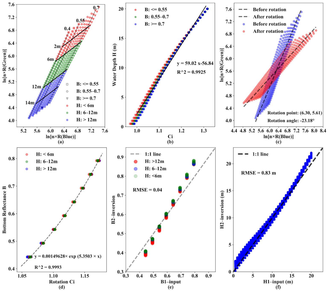
2.1. Basic Model
2.2. Model Checking Using Hydrolight Simulation Dataset
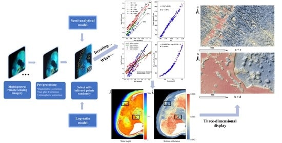
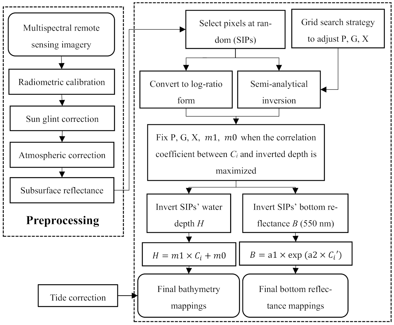
2.3. Workflow
3. Case Study
3.1. Study Area, In-Situ Water Depth Data and Benthic Mapping
3.2. Satellite Images
3.3. Preprocessing of the Images
3.3.1. Sun Glint Correction
3.3.2. Atmospheric Correction
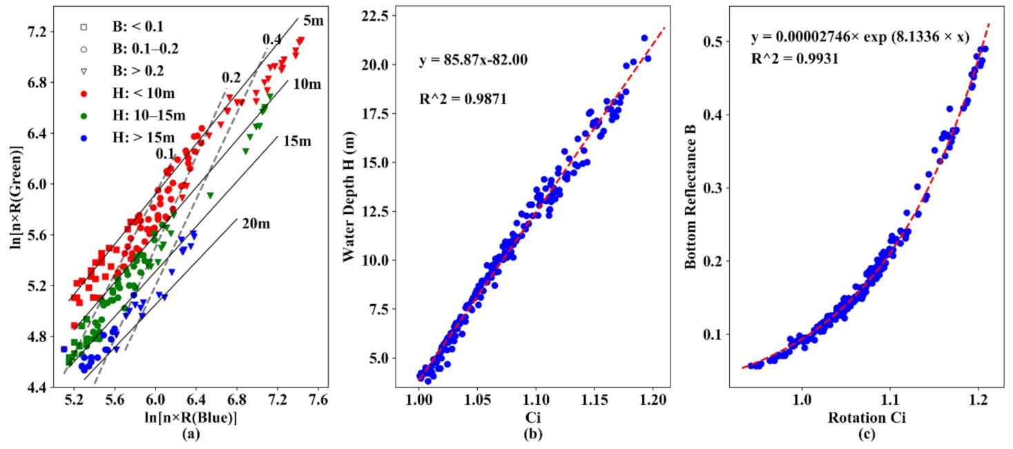
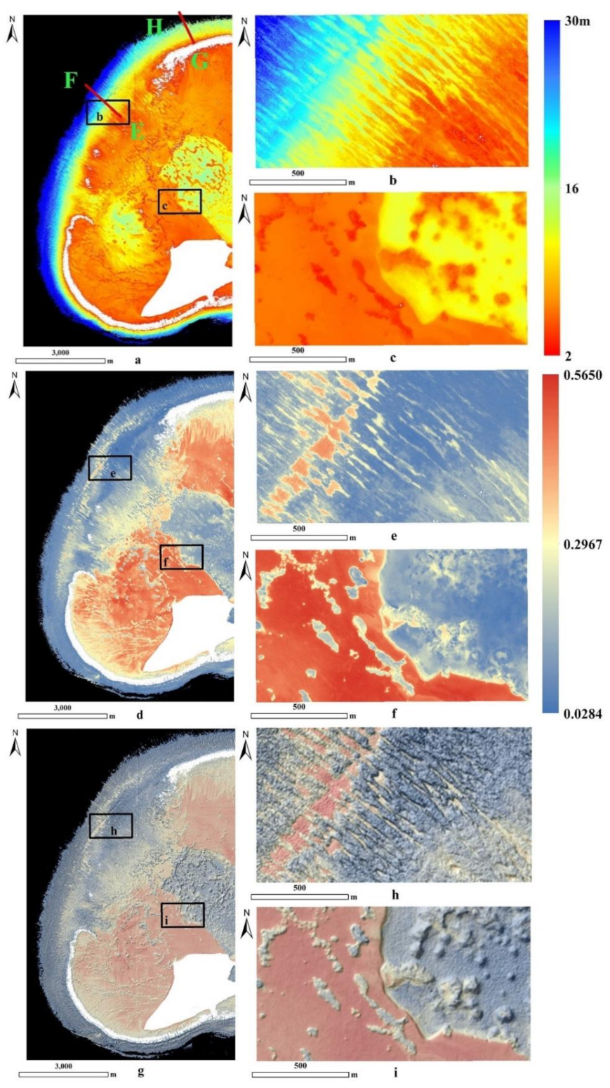
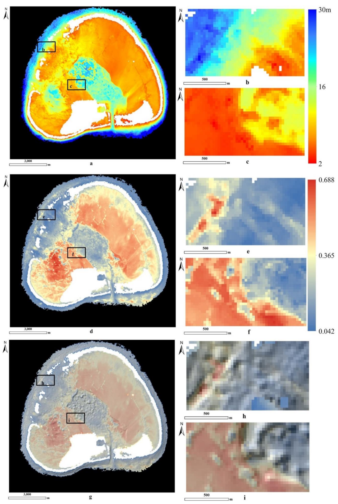
3.4. Inversion of Bottom Reflectance and Water Depth
4. Discussion
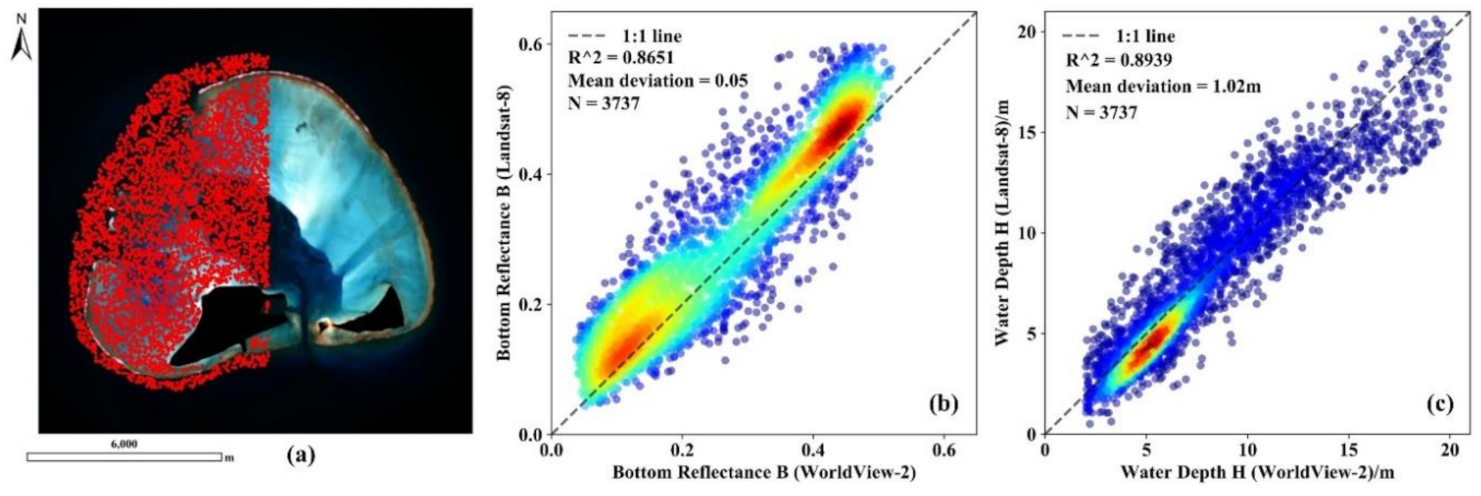
4.1. Cross-Checking Using WorldView-2 and Landsat-8 Images
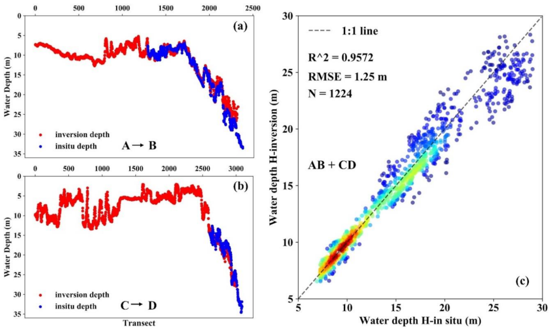
4.2. Indirect Checking Using In-Situ Water Depth Data
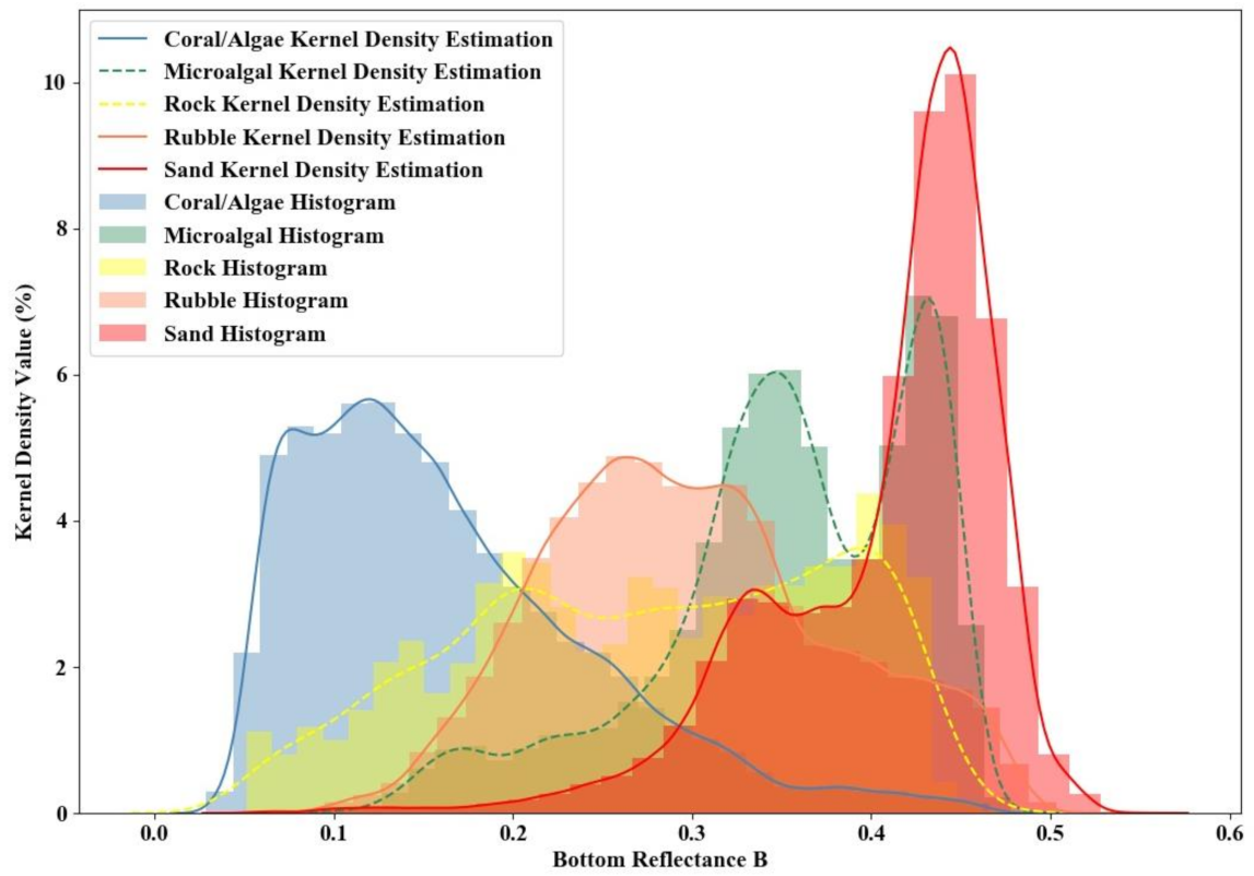
4.3. Indication of the Bottom Reflectance for Benthic Habitat Mapping
4.4. Inversion Ranges under Different Bottom Reflectance
5. Conclusions
Author Contributions
Funding
Institutional Review Board Statement
Informed Consent Statement
Data Availability Statement
Acknowledgments
Conflicts of Interest
Appendix A
Appendix B

| Variable | Inputs |
|---|---|
| Particle phase function | Petzold average particle |
| Inelastic scattering | Ignore |
| Chlorophyl a [chl-a](mg/m3) | 0.05, 0.1, 0.15, 0.2 |
| B (550 nm): ooid_sand | 0.44, 0.49, 0.54, 0.59, 0.64, 0.69, 0.74, 0.79 |
| H: water depth | 0.5–20 m, every 0.5 m |
| λ | 400–700 nm, every 10 nm |
| Sea surface wind speed | 5 m/s |
| Salinity | 0.035 |
| Solar zenith angle | 30° |


References
- Petit, T.; Bajjouk, T.; Mouquet, P.; Rochette, S.; Vozel, B.; Delacourt, C. Hyperspectral remote sensing of coral reefs by semi-analytical model inversion—Comparison of different inversion setups. Remote Sens. Environ. 2017, 190, 348–365. [Google Scholar] [CrossRef]
- Heron, S.F.; Johnston, L.; Liu, G.; Geiger, E.F.; Maynard, J.A.; De La Cour, J.L.; Johnson, S.; Okano, R.; Benavente, D.; Burgess, T.F.R.; et al. Validation of reef-scale thermal stress satellite products for coral bleaching monitoring. Remote Sens. 2016, 8, 59. [Google Scholar] [CrossRef]
- Awak, D.S.H.; Gaol, J.L.; Subhan, B.; Madduppa, H.H.; Arafat, D. Coral reef ecosystem monitoring using remote sensing data: Case study in Owi Island, Biak, Papua. Procedia Environ. Sci. 2016, 33, 600–606. [Google Scholar] [CrossRef]
- Hedley, J.; Roelfsema, C.; Chollett, I.; Harborne, A.; Heron, S.; Weeks, S.; Skirving, W.; Strong, A.; Eakin, C.; Christensen, T.; et al. Remote sensing of coral reefs for monitoring and nanagement: A review. Remote Sens. 2016, 8, 118. [Google Scholar] [CrossRef]
- Zhang, C. Applying data fusion techniques for benthic habitat mapping and monitoring in a coral reef ecosystem. ISPRS J. Photogramm. Remote Sens. 2015, 104, 213–223. [Google Scholar] [CrossRef]
- Misiuk, B.; Brown, C.J.; Robert, K.; Lacharité, M. Harmonizing multi-source sonar backscatter datasets for seabed mapping using bulk shift approaches. Remote Sens. 2020, 12, 601. [Google Scholar] [CrossRef]
- Janowski, L.; Madricardo, F.; Fogarin, S.; Kruss, A.; Molinaroli, E.; Kubowicz-Grajewska, A.; Tegowski, J. Spatial and temporal changes of tidal inlet using object-based image analysis of multibeam echosounder measurements: A case from the Lagoon of Venice, Italy. Remote Sens. 2020, 12, 2117. [Google Scholar] [CrossRef]
- Chen, B.; Yang, Y.; Xu, D.; Huang, E. A dual band algorithm for shallow water depth retrieval from high spatial resolution imagery with no ground truth. ISPRS J. Photogramm. Remote Sens. 2019, 151, 1–13. [Google Scholar] [CrossRef]
- Dong, Y.; Liu, Y.; Hu, C.; Xu, B. Coral reef geomorphology of the Spratly Islands: A simple method based on time-series of Landsat-8 multi-band inundation maps. ISPRS J. Photogramm. Remote Sens. 2019, 157, 137–154. [Google Scholar] [CrossRef]
- Sandidge, J.C.; Holyer, R.J. Coastal bathymetry from hyperspectral observations of water radiance. Remote Sens. Environ. 1998, 65, 341–352. [Google Scholar] [CrossRef]
- Purkis, S.J.; Gleason, A.C.R.; Purkis, C.R.; Dempsey, A.C.; Renaud, P.G.; Faisal, M.; Saul, S.; Kerr, J.M. High-resolution habitat and bathymetry maps for 65,000 sq. km of Earth’s remotest coral reefs. Coral Reefs 2019, 38, 467–488. [Google Scholar] [CrossRef]
- Collin, A.; Archambault, P.; Planes, S. Revealing the regime of shallow coral reefs at patch scale by continuous spatial modeling. Front. Mar. Sci. 2014, 1, 65. [Google Scholar] [CrossRef]
- Reichstetter, M.; Fearns, P.R.C.S.; Weeks, S.J.; McKinna, L.I.W.; Roelfsema, C.; Furnas, M. Bottom reflectance in ocean color satellite remote sensing for coral reef environments. Remote Sens. 2015, 7, 16756–16777. [Google Scholar] [CrossRef]
- Li, J.; Schill, S.R.; Knapp, D.E.; Asner, G.P. Object-based mapping of coral reef habitats using planet dove satellites. Remote Sens. 2019, 11, 1445. [Google Scholar] [CrossRef]
- Roelfsema, C.; Kovacs, E.; Ortiz, J.C.; Wolff, N.H.; Callaghan, D.; Wettle, M.; Ronan, M.; Hamylton, S.M.; Mumby, P.J.; Phinn, S. Coral reef habitat mapping: A combination of object-based image analysis and ecological modelling. Remote Sens. Environ. 2018, 208, 27–41. [Google Scholar] [CrossRef]
- O’Neill, J.D.; Costa, M.; Sharma, T. Remote sensing of shallow coastal benthic substrates: In situ spectra and mapping of eelgrass (zostera marina) in the gulf islands national park reserve of Canada. Remote Sens. 2011, 3, 975–1005. [Google Scholar] [CrossRef]
- Lyzenga, D.R. Passive remote sensing techniques for mapping water depth and bottom features. Appl. Opt. 1978, 17, 379–383. [Google Scholar] [CrossRef] [PubMed]
- Lee, Z.; Carder, K.L.; Mobley, C.D.; Steward, R.G.; Patch, J.S. Hyperspectral remote sensing for shallow waters I A semianalytical model. Appl. Opt. 1998, 37, 6329–6338. [Google Scholar] [CrossRef] [PubMed]
- Lee, Z.; Carder, K.L.; Mobley, C.D.; Steward, R.G.; Patch, J.S. Hyperspectral remote sensing for shallow waters: 2 Deriving bottom depths and water properties by optimization. Appl. Opt. 1999, 38, 3831–3843. [Google Scholar] [CrossRef] [PubMed]
- Lee, Z.; Carder, K.L.; Chen, R.F.; Peacock, T.G. Properties of the water column and bottom derived from Airborne Visible Infrared Imaging Spectrometer (AVIRIS) data. J. Geophys. Res. Space Phys. 2001, 106, 11639–11651. [Google Scholar] [CrossRef]
- Casey, B.; Lee, Z.; Arnone, R.A.; Weidemann, A.D.; Parsons, R.; Montes, M.J.; Gao, B.-C.; Goode, W.; Davis, C.O.; Dye, J. Water and bottom properties of a coastal environment derived from Hyperion data measured from the EO-1 spacecraft platform. J. Appl. Remote Sens. 2007, 1, 011502. [Google Scholar] [CrossRef]
- Dekker, A.G.; Phinn, S.R.; Anstee, J.M.; Bissett, P.; Brando, V.E.; Casey, B.; Fearns, P.; Hedley, J.; Klonowski, W.; Lee, Z.P.; et al. Intercomparison of shallow water bathymetry, hydro-optics, and benthos mapping techniques in Australian and Caribbean coastal environments. Limnol. Oceanogr. Methods 2011, 9, 396–425. [Google Scholar] [CrossRef]
- Manessa, M.D.M.; Kanno, A.; Sagawa, T.; Sekine, M.; Nurdin, N. Simulation-based investigation of the generality of Lyzenga’s multispectral bathymetry formula in Case-1 coral reef water. Estuar. Coast. Shelf Sci. 2018, 200, 81–90. [Google Scholar] [CrossRef]
- Figueiredo, I.N.; Pinto, L.; Goncalves, G. A modified Lyzenga’s model for multispectral bathymetry using Tikhonov regularization. IEEE Geosci. Remote Sens. Lett. 2015, 13, 53–57. [Google Scholar] [CrossRef]
- Ohlendorf, S.; Müller, A.; Heege, T.; Cerdeira-Estrada, S.; Kobryn, H.T. Bathymetry mapping and sea floor classification using multispectral satellite data and standardized physics-based data processing. In Proceedings of the Remote Sensing of the Ocean, Sea Ice, Coastal Waters, and Large Water Regions 2011, Prague, Czech Republic, 21–22 September 2011; SPIE: Washington, DC, USA, 2011; Volume 8175, p. 817503. [Google Scholar]
- Eugenio, F.; Marcello, J.; Martin, J. High-resolution maps of bathymetry and benthic habitats in shallow-water environments using multispectral remote sensing imagery. IEEE Trans. Geosci. Remote Sens. 2015, 53, 3539–3549. [Google Scholar] [CrossRef]
- Niroumand-Jadidi, M.; Pahlevan, N.; Vitti, A. Mapping substrate types and compositions in shallow streams. Remote Sens. 2019, 11, 262. [Google Scholar] [CrossRef]
- Katja, D.; Anna, G.; Peter, G.; Bringfried, P.; Natascha, O. Water constituents and water depth retrieval from sentinel-2a—A first evaluation in an oligotrophic lake. Remote Sens. 2016, 8, 941. [Google Scholar]
- Niroumand-Jadidi, M.; Bovolo, F.; Bruzzone, L.; Gege, P. Physics-based bathymetry and water quality retrieval using planetscope imagery: Impacts of 2020 COVID-19 lockdown and 2019 extreme flood in the Venice Lagoon. Remote Sens. 2020, 12, 2381. [Google Scholar] [CrossRef]
- Stumpf, R.P.; Holderied, K.; Sinclair, M. Determination of water depth with high-resolution satellite imagery over variable bottom types. Limnol. Oceanogr. 2003, 48, 547–556. [Google Scholar] [CrossRef]
- Mobley, C.D. Hydrolight 3.0 Users’ Guide; Final Report; Project 5632; SRI~SRI International: Menlo Park, CA, USA, 1995. [Google Scholar]
- Li, J.; Knapp, D.E.; Schill, S.R.; Roelfsema, C.; Phinn, S.; Silman, M.; Mascaro, J.; Asner, G.P. Adaptive bathymetry estimation for shallow coastal waters using Planet Dove satellites. Remote Sens. Environ. 2019, 232, 111302. [Google Scholar] [CrossRef]
- Boyce, D.G.; Lewis, M.R.; Worm, B. Global phytoplankton decline over the past century. Nat. Cell Biol. 2010, 466, 591–596. [Google Scholar] [CrossRef]
- Gao, H.; Zhao, H.; Shen, C.Y. Progress in ocean color remote sensing of Chinese marginal seas. Int. J. Ecol. 2017, 6, 82–92. [Google Scholar] [CrossRef]
- Henson, S.A.; Sarmiento, J.L.; Dunne, J.P.; Bopp, L.; Lima, I.; Doney, S.C.; John, J.; Beaulieu, C. Detection of anthropogenic climate change in satellite records of ocean chlorophyll and productivity. Biogeosciences 2010, 7, 621–640. [Google Scholar] [CrossRef]
- Mobley, C.D. Light and Water: Radiative Transfer in Natural Waters; Academic Press: New York, NY, USA, 1994. [Google Scholar]
- Xia, H.; Li, X.; Zhang, H.; Wang, J.; Lou, X.; Fan, K.; Shi, A.; Li, D. A bathymetry mapping approach combining log-ratio and semianalytical models using four-band multispectral imagery without ground data. IEEE Trans. Geosci. Remote Sens. 2020, 58, 2695–2709. [Google Scholar] [CrossRef]
- Chavez, P.S.J. Image-based atmospheric corrections revisited and improved. Photogram. Eng. Remote Sens. 1996, 62, 1025–1036. [Google Scholar]
- Liang, S.; Fallah-Adl, H.; Kalluri, S.; Jájá, J.; Kaufman, Y.J.; Townshend, J.R.G. An operational atmospheric correction algorithm for Landsat Thematic Mapper imagery over the land. J. Geophys. Res. Space Phys. 1997, 102, 17173–17186. [Google Scholar] [CrossRef]
- Song, C.; Woodcock, C.E.; Seto, K.C.; Lenney, M.P.; Macomber, S.A. Classification and change detection using Landsat tm data: When and how to correct atmospheric effects? Remote Sens. Environ. 2001, 75, 230–244. [Google Scholar] [CrossRef]
- Egbert, G.D.; Erofeeva, Y. Efficient inverse modeling of barotropic ocean tides. J. Atmos. Ocean. Technol. 2002, 19, 183–204. [Google Scholar] [CrossRef]
- Brown, C.J.; Smith, S.J.; Lawton, P.; Anderson, J.T. Benthic habitat mapping: A review of progress towards improved understanding of the spatial ecology of the seafloor using acoustic techniques. Estuar. Coast. Shelf Sci. 2011, 92, 502–520. [Google Scholar] [CrossRef]
- Lecours, V.; Devillers, R.; Schneider, D.C.; Lucieer, V.L.; Brown, C.J.; Edinger, E.N. Spatial scale and geographic context in benthic habitat mapping: Review and future directions. Mar. Ecol. Prog. Ser. 2015, 535, 259–284. [Google Scholar] [CrossRef]
- Liu, Z. Bathymetry and bottom albedo retrieval using Hyperion: A case study of Thitu Island and reef. Chin. J. Oceanol. Limnol. 2013, 31, 1350–1355. [Google Scholar] [CrossRef]


Publisher’s Note: MDPI stays neutral with regard to jurisdictional claims in published maps and institutional affiliations. |
© 2021 by the authors. Licensee MDPI, Basel, Switzerland. This article is an open access article distributed under the terms and conditions of the Creative Commons Attribution (CC BY) license (http://creativecommons.org/licenses/by/4.0/).
Share and Cite
Ma, Y.; Zhang, H.; Li, X.; Wang, J.; Cao, W.; Li, D.; Lou, X.; Fan, K. An Exponential Algorithm for Bottom Reflectance Retrieval in Clear Optically Shallow Waters from Multispectral Imagery without Ground Data. Remote Sens. 2021, 13, 1169. https://doi.org/10.3390/rs13061169
Ma Y, Zhang H, Li X, Wang J, Cao W, Li D, Lou X, Fan K. An Exponential Algorithm for Bottom Reflectance Retrieval in Clear Optically Shallow Waters from Multispectral Imagery without Ground Data. Remote Sensing. 2021; 13(6):1169. https://doi.org/10.3390/rs13061169
Chicago/Turabian StyleMa, Yunhan, Huaguo Zhang, Xiaorun Li, Juan Wang, Wenting Cao, Dongling Li, Xiulin Lou, and Kaiguo Fan. 2021. "An Exponential Algorithm for Bottom Reflectance Retrieval in Clear Optically Shallow Waters from Multispectral Imagery without Ground Data" Remote Sensing 13, no. 6: 1169. https://doi.org/10.3390/rs13061169
APA StyleMa, Y., Zhang, H., Li, X., Wang, J., Cao, W., Li, D., Lou, X., & Fan, K. (2021). An Exponential Algorithm for Bottom Reflectance Retrieval in Clear Optically Shallow Waters from Multispectral Imagery without Ground Data. Remote Sensing, 13(6), 1169. https://doi.org/10.3390/rs13061169