Article

Satellite-Observed Global Terrestrial Vegetation Production in Response to Water Availability

1
State Key Laboratory of Urban and Regional Ecology, Research Center for Eco-Environmental Sciences, Chinese Academy of Sciences, Beijing 100085, China
2
University of Chinese Academy of Sciences, Beijing 100049, China
3
School of Land Engineering, Chang’an University, Xi’an 710054, China
*
Author to whom correspondence should be addressed.
Remote Sens. 2021, 13(7), 1289; https://doi.org/10.3390/rs13071289
Submission received: 7 March 2021 / Revised: 21 March 2021 / Accepted: 25 March 2021 / Published: 28 March 2021
(This article belongs to the Special Issue Remote Sensing in Hydrology and Water Resources Management)

Abstract

:
Water stress is one of the primary environmental factors that limits terrestrial ecosystems’ productivity. Hense, the way to quantify gobal vegetation productivity’s vulnerability under water stress and reveal its seasonal dynamics in response to drought is of great significance in mitigating and adapting to global changes. Here, we estimated monthly gross primary productivity (GPP) first based on light-use efficiency (LUE) models for 1982–2015. GPP’s response time to water availability can be determined by correlating the monthly GPP series with the multiple timescale Standardized Precipitation Evapotranspiration Index (SPEI). Thereafter, we developed an optimal bivariate probabilistic model to derive the vegetation productivity loss probabilities under different drought scenarios using the copula method. The results showed that LUE models have a good fit and estimate GPP well (R2 exceeded 0.7). GPP is expected to decrease in 71.91% of the global land vegetation area because of increases in radiation and temperature and decreases in soil moisture during drought periods. Largely, we found that vegetation productivity and water availability are correlated positively globally. The vegetation productivity in arid and semiarid areas depends considerably upon water availability compared to that in humid and semi-humid areas. Weak drought resistance often characterizes the land cover types that water availability influences more. In addition, under the scenario of the same level of GPP damage with different drought degrees, as droughts increase in severity, GPP loss probabilities increase as well. Further, under the same drought severity with different levels of GPP damage, drought’s effect on GPP loss probabilities weaken gradually as the GPP damage level increaes. Similar patterns were observed in different seasons. Our results showed that arid and semiarid areas have higher conditional probabilities of vegetation productivity losses under different drought scenarios.

1. Introduction

The Intergovernmental Panel on Climate Change (IPCC) report shows that the world will continue to warm in the 21st century [1]. This indicates that as the future temperature rises, the occurrence and frequency of extreme weather and climate, such as heatwaves and droughts, will increase rapidly [2]. This trend and its associated adverse effects on natural and social ecosystems are expected to increase further [3]. Terrestrial ecosystems’ gross primary productivity (GPP) is the largest component of global terrestrial carbon flux, and slight fluctuations in GPP have a significant influence on atmospheric CO2 concentration [4]. On a global scale, particularly in arid and semiarid regions, water stress is the primary environmental factor that limits terrestrial ecosystems’ productivity [5]. Hence, studying drought’s effects on their productivity has become an important priority in global change research.
The terrestrial ecosystem’s productivity characterizes its quality, it is the key to controlling the ecosystem’s carbon, water, energy and nutrient cycles, and plays a decisive role in regulating its function and controlling its carbon source and sink [6]. At the same time, ecosystem productivity is also the basis of a variety of ecosystem services [7] and is the source of food, fiber, wood, livestock grains and biofuels in human society [8]. As the main outcome and important manifestation of global climate change, drought not only affects photosynthesis and ecosystem productivity directly [9], but it can also affect terrestrial ecosystem productivity in directly by changing the intensity and frequency of other forms of disturbance, such as increasing the frequency and intensity of fires, plant mortality and the occurrence of pests and diseases [10]. In recent years, many studies have investigated drought’s effects on terrestrial ecosystems’ productivity at different spatio-temporal scales based on long-term observations from ecological research sites, field experiments, eddy covariance measurements, large-scale satellite measurements and model simulations [11,12,13]. Satellites data used commonly to evaluate vegetation productivity include primarily the Moderate Resolution Imaging Spectroradiometer-Fraction of Photosynthetically Active Radiation (MODIS-FPAR) and the Global Inventory Modeling and Mapping Studies-Fraction of Photosynthetically Active Radiation (AVHRR GIMMS-FPAR), remotely-sensed data for atmosphere state, MODIS Enhanced Vegetation Index, leaf area index, spatially distributed CO2 concentrations, and canopy information. For example, Reichstein et al. [11] found that the drought stress in Europe in summer 2003 caused the reduction of ecosystem productivity by jointing flux tower, remote sensing (including MODSI and AVHRR-GIMMS FPAR) and modelling datasets. Zhang et al. [14] emphasized that the drought in Southwestern China in spring 2010 reduced primary productivity by using primary productivity products derived from MODIS. Stocker et al. [15] used four remote sensing data-driven models and demenstrated that drought’s effects on terrestrial primary production were underestimated. Previous studies have shown that different vegetation types and environmental conditions (such as climate and soil factors) largely determine biological communities’ resistance and ability to recover from drought stress [16].
Although there is increasing recognition of drought’s adverse effects on terrestrial vegetation productivity, few studies have focused on the seasonal dynamics in global productivity in response to drought across various climate zones and land biomes. Moreover, studies of drought’s lag effect on terrestrial vegetation productivity and vegetation’s responses to drought at various time-scales on a global scale are scare. The Standardized Precipitation Evapotranspiration Index (SPEI) quantifies different drought types based on the water balance, and is used widely on global and regional scales because of its multiple time scales and spatial comparability [17]. Therefore, determining the corresponding time scale when GPP and SPEI have the highest correlation based upon different time scales is of great significance in understanding the variations in different terrestrial ecosystems’ productivity depending uopn drought resistance. In addition, we give greater attention here to the way to quantify the probability of varying degrees of damage to vegetation productivity under predictable drought scenarios. Copulas can be used to couple multiple variables and construct their joint probability distribution by considering their correlations [18], which can derive the vegetation productivity loss distributions conditioned on any drought scenario. For example, Madadgar et al. [19] estimated the probability of drought in agricultural production in Australia based on a copula model, while Fang et al. [20] constructed a bivariate probabilistic framework to assess vegetation vulnerability and map drought-prone ecosystems in China’s Loess Plateau.
Given ecosystem productivity’s key role in affecting the global carbon budget and the supply of ecosystem services, in the context of global warming, the rapid increase in atmospheric carbon dioxide concentration, and increasing human food production and resource demand, estimating ecosystem productivity accurately is important to assess drought’s effects on terrestrial ecosystems precisely [21]. Three main methods are used to estimate ecosystems’ productivity at the regional and global scales—remote sensing-based light-use efficiency (LUE) models [22], machine learning algorithms [23], and process-based physiological and ecological models [24]. Remote sensing observations can provide information continuously on land surface features that affect ecosystem productivity, such as ecosystem structure, vegetation phenology, biomass, soil moisture, and land cover over a large area. The LUE model relies on remote sensing observation data to estimate ecosystem productivity through the utilization rate of photosynthetically active radiation in the ecosystem [25]. We gave special attention to determining water stress and produced a data set of monthly LUE GPPs at the global scale based on various representations of water stress: Water stress based on vapor-pressure deficit, humidity deficit and root-zone soil-water content separately.
Our study had two primary objectives. The first was to determine the seasonal dynamics of global vegetation productivity’s response to drought across various climate zones and land biomes, and the second was to quantify the probability of varying degrees of damage to vegetation productivity under predictable drought scenarios. First, we used a LUE model to produce a dataset of global monthly satellite-observed GPPs, which are designed primarily to determinate water stress. Second, we explored vegetation productivity’s spatio-temporal evolution of dependence and response time to water availability by correlating monthly GPP series with the multiple timescale SPEIs (1- to 24-months). Finally, we develpoed an optimal bivariate probabilistic model in each pixel of the globe using the copula method, which was used to derive the vegetation productivity loss probabilities under different drought scenarios.

2. Materials and Methods

2.1. Data

2.1.1. Remote Sensing Data

The actual evapotranspiration, potential evapotranspiration and soil moisture (including surface soil and root-zone soil moisture) data were derived from the Global Land Evaporation Amsterdam Model (GLEAM), which is designed to be determined by remote sensing observations only [26]. The GLEAM_V3.3a dataset has a 0.25° spatial resolution at a monthly time step that spans the 39-year period from 1980–2018 (www.gleam.eu (accessed on 25 March 2021)). Fraction of Photosynthetically Active Radiation (FPAR)3g data were generated from AVHRR GIMMS NDVI3g using an Artificial Neural Network (ANN) derived model, with a spatial resolution of 1/12° and a 15 days time interval [27]. We used the MODIS MCD12C1 product, which contains yearly, worldwide distributions of 17 land cover types from 2001–2017 at a spatial resolution of 0.05° (https://lpdaac.usgs.gov/ (accessed on 10 December 2020)) [28]. In this study, barren land, water bodies, permanent snow, and ice were removed.

2.1.2. Meteorological data and FLUXNET data

Downward shortwave radiation, air temperature, specific humidity and air pressure were obtained from the CRU-NCEPV6.1 dataset with a spatial resolution of 0.5° and a 6-h time interval. We used gross primary productivity (GPP) data from the FLUXNET2015 dataset to compare flux site measurement of GPP and LUE GPP (https://fluxnet.org/data/fluxnet2015-dataset/ (accessed on 1 December 2020)).

2.2. Drought Index

SPEI can be calculated by fitting the difference between precipitation and potential evapotranspiration based on a log-logistic probability distribution, which combines the multi-temporal characteristic of standardized precipitation index and the sensitivity of palmer drought severity index to changes in evaporation demand. A global gridded dataset of the SPEI was calculated using monthly precipitation and potential evapotranspiration from the CRU TS3.24.01 dataset [29]. This dataset is generated at a 0.5° spatial resolution and at a monthly time step and covers the period from 1902 to 2015. We used the SPEI dataset from 1982 to 2015 in this study, which contains timescales from 1- to 24-months. A 6-month SPEI value is formulated by the cumulative water deficit or surplus from five months before to the current month. Three drought scenarios including moderate (−1.5 < SPEI ≤ 1), severe (−2 < SPEI ≤ −1.5), and extreme (SPEI ≤ −2) can be differentiated using a set of SPEI thresholds [29]. The yearly aridity index (AI), which has a spatial resolution of 0.5°, was calculated with Feng and Fu’s formula [30]. (Response: we cited the citation 31 in Section 2.3) According to this dataset, global land can be classified into arid (0.05 ≤ AI < 0.2), semiarid (0.2 ≤ AI < 0.5), semihumid (0.5 ≤ AI < 0.65) and humid zones (AI ≥ 0.65).

2.3. LUE GPP

The global GPP for the 1982–2015 period was calculated based on the LUE equation, as follows [31]:
G P P = ε m a x × S O L × 0.45 × f P A R × f ( T ) × f ( W ) ,
in which ε m a x is vegetation type related maximum light use efficiency, S O L is downward solar shortwave radiation, and f P A R represents the fraction of photosynthetically active radiation vegetation absorbs. f t and f w are temperature and water stress respectively to plant productivity. We adopted the meteorological data from the CRU-NCEPV6.1 dataset, which includes downward shortwave radiation, air temperature, specific humidity and air pressure, and so forth. We used f P A R Zhu et al. [27] developed. We calculated the temperature stress with Equation (2), as follows:
f t = ( T T M I N ) ( T T M A X ) [ ( T T M I N ) ( T T M A X ) ] ( T T o p t ) 2 ,
in which T M I N and T M A X are the minimum and maximum temperature for plant’s photosynthesis, with the specific parameters can be found in Zhang et al. [32].
In this study, we focused particularly on determining water stress ( f w ) in the LUE equation. The MODIS-GPP algorithm [33] calculates f w with the daily vapor pressure deficit (VPD) on consideration that leaf stomatal conductance is mainly restricted by cold stress and VPD, named VPDMOD expressed as in Equation (3):
f w = f ( V P D ) = { 1               V P D V P D o p e n V P D c l o s e V P D V P D c l o s e V P D o p e n                 V P D o p e n < V P D < V P D c l o s e 0                 V P D V P D c l o s e ,
in which V P D c l o s e represents VPD that induces full stomatal closure, while V P D o p e n represents VPD that results in full stomatal opening, all parameters are set based on the vegetation type.
The GLO-PEM algorithm [34] considers each vegetation type’s optimum growth temperature ( T o p t ). The algorithm calculates water stress with vegetation type, independently with Equation (4) named VPDGLO:
f w = f ( V P D ) = { 1 0.05 δ q                   0 < δ q 15 0.25                 δ q > 15 ,
in which δ q is the specific humidity deficit (g/kg), the difference between saturated and actual specific humidity.
The CASA model provides a framework that considers water stress with a multidisciplinary algorithm [35], shown in Equation (5), as follows:
f w = f ( V P D ) × W s W s = { 1   V P D   o n l y   m o d e l 0.5 + E T R   V P D + E T R   m o d e l 0.5   +   K S   V P D + S M   m o d e l ,
in which E T R is the ratio of actual evapotranspiration to potential evapotranspiration. According to FAO 56 [36], E T R can be equal to K S , which is calculated based on root zone soil moisture (hereinafter S M ) and soil and vegetation properties, written as Equations (6) and (7):
  K S = S M W P ( 1 p ) × T A W
p = p s t d + 0.04 × ( 5 E T 0 ) ,
in which WP and T A W represent soil wilting point and total available soil water derived from the International Geosphere-Biosphere Programme Data and Information System (IGMP-DIS) dataset [37] and the World Inventory of Soil property Estimates (WISE) derived soil properties [38]. E T 0 is calculated with Hagreaves equation [39] while p s t d is a vegetation type-specific depletion factor (allowable extent of soil water deficit before water stress) at E T 0 of 5 mm per day. Actual evapotranspiration, potential evapotranspiration, and root-zone soil moisture data were all acquired from the GLEAM dataset.
In this study, we provided a dataset of monthly plant productivity that spans the 34-year period from 1982–2015 at the global scale, composed by five LUE GPPs derived from the multidisciplinary framework in Equation (5). These five GPPs represent different considerations of water stress in the LUE equation, the VPD only model, VPDGLO-ETR model, VPDMOD-ETR model, VPDGLO-SM model, and VPDMOD-SM model. Because the LUE equation estimate GPP from multiple satellite data, for example, NDVI, FPAR, and GLEAM soil water, it is considered satellite-observed GPP.

2.4. Determining LUE GPP’s Response Time to Water Availability

To screen out vegetation productivity’s response time to water availability, a monthly GPP series from 1982 to 2015 was correlated with the multiple timescale SPEI (1- to 24-months). For the i-th month in a year, Spearman’s correlation analysis was performed between the monthly GPP and SPEI series at different timescales as follows
R j i = c o r r ( G P P i , S P E I j i )   i = 1 ,   2   , , 12 ,   j = 1 ,   2 , , 24 ,
in which R is the correlation coefficient and a timescale j denotes the cumulative water deficit or surplus from j-1 months before to the current month. Finally, a timescale able to maximize the GPP-SPEI association, is retained as the vegetation productivity response time (VPRT) to water variations for the i-th month.
V P R T i = m a x { R j i }   j = 1 ,   2 ,   ,   24 .

2.5. Copulas

We chose the extreme value (EV), generalized extreme value (GEV), exponential (EXP), gamma (GAM), Poisson (POISS), normal (NOR), generalized Pareto (GP) and Weibull (WBL) distribution functions to fit the monthly GPP series (Table S1). The SPEI series is a statistic distributed normally and accordingly, the normal distribution is employed as its marginal. The probability distribution functions of monthly GPP and SPEI series are defined as FGPP (gpp) and FSPEI (spei), respectively.
We constructed a joint distribution function in each pixel of the globe in every month based on monthly GPP and SPEI series. Considering FGPP (gpp) and FSPEI (spei), these two marginal distribution’s joint distribution function can be defined as a copula C:
F G P P , S P E I ( g p p , s p e i ) = C ( F G P P ( g p p ) , F S P E I ( s p e i ) ) .
In this study, we used the methods of maximum likelihood and inference functions for margins to estimate the fitted parameters in FGPP (gpp), FSPEI (spei) and FGPP,SPEI (gpp, spei) [40]. The bivariate distribution functions used commonly, including the Frank, Clayton, Gumbel, t and Normal copulas, were constructed to couple FGPP (gpp)) and FSPEI (spei) in each pixel of the globe (as shown in Table S2).
Next, we obtained the optimal joint distribution function of FGPP (gpp) and FSPEI (spei) as follows by referring to the method of the goodness-of-fit test Zhang et al. [41] provided.
F G P P , S P E I ( g p p , s p e i ) = P ( G P P g p p , S P E I s p e i ) = g p p s p e i f ( g p p , s p e i ) d u d v .
Ultimately, we generated a set of conditional probabilities of vegetation productivity losses for diverse drought conditions with a bivariate statistical framework. Larger values of vegetation productivity loss probabilities under the same scenario imply greater ecosystem vulnerability, and such ecosystems are categorized thereby as the drought-prone class. Given multiple drought scenarios, conditional probabilities of vegetation productivity lower than different percentiles (e.g., the 10th, 20th, 30th, 40th percentiles were considered in the study) are derived using copula-based joint distribution and the conditional distribution formulas. The conditional probabilities of different percentiles of vegetation productivity loss under moderate, severe and extreme drought scenarios can be calculated by the following formula.
P ( G P P < g p p |   1.5 < S P E I 1 ) = F G P P ,   S P E I ( g p p , 1 ) F G P P ,   S P E I ( g p p ,   1.5 ) F S P E I ( 1 ) F S P E I ( 1.5 )
P ( G P P < g p p | 2 < S P E I 1.5 ) = F G P P ,   S P E I ( g p p , 1.5 ) F G P P ,   S P E I ( g p p ,   2 ) F S P E I ( 1.5 ) F S P E I ( 2 )
P ( G P P < g p p |   S P E I 2 ) = F G P P ,   S P E I ( g p p , 2 ) F S P E I ( 2 ) .

2.6. Statistical Tests

We used the linear regression method to calculate the GPP’s mean change rate over the entire temporal domain. A two-tailed t-test and the Mann-Kendall test were used to examine the significance of the trend, while the Kolmogorov–Smirnov test was used to establish the optimal marginal distribution function of GPP (p < 0.05). In addition, we adopted several goodness-of-fit measures to evaluate different copula models’ performance, including the squared Euclidean distance (SED) between the theoretical copula and the empirical copula, the root mean squared error (RMSE) and the Akaike information criterion (AIC).

3. Results

3.1. Validation of LUE GPPs’ Accuracy, Dynamics Trends and Drought’s Effect on GPP

In this study, special attention was given to determining water stress (including atmosphere vapor pressure deficit, soil moisture content and the humidity deficit) in the LUE model to estimate the global GPP. By comparing with the FLUXNET GPP site data, we found that different LUE models have a good fit in estimation of LUE GPP. The fitted R2 of VPDGLO-SM, VPDMOD-SM, VPDGLO-ETR, and VPDMOD-ETR were 0.7739, 0.7399, 0.7427, 0.7459 and 0.7628, respectively (Table 1). The average goodness of fit of multiple models reached 0.78 (Figure S2). Overall, LUE GPP had a greater response to the atmospheric vapor pressure deficit, followed by soil water content, and the humidity deficit. The LUE GPP showed greater sensitivity to soil moisture content than the vapor pressure deficit only in evergreen needleleaf forest (ENF), mixed forest (MF) (R2 = 0.7833 and 0.8479, respectively, RMSE = 1.6399 and 1.3825, respectively). The annual average spatial distribution of GPP in multiple models is shown in Figure S1. From 1982 to 2015, the global average annual GPP of terrestrial vegetation continued to increase at a mean rate of 0.134 Pg C a −1 (p < 0.001), but its growth rate declined after the mid-1990s (Figure 1a). From the spatial distribution of the mean annual GPP change trend, it can be seen that the global mean annual GPP still had a largely increasing trend, and the significant increase area accounted for 36.83% of the global terrestrial vegetation area, located primarily in the mid-high latitudes of the northern hemisphere, India, Southeastern China, Southeastern South America, Northern and Southern Africa, and Eastern Australia. 11.62% of the regional GPP showed a significant downward trend, largely in Eastern Brazil and Central and Southern Africa (Figure 1b).
Taking SPEI-12 as an example, a drought episode with an SPEI value less than −1 and no less than 3 consecutive months was considered a drought event. We counted the total frequency of droughts from 1982 to 2015 in each grid around the world. It can be seen that the global drought-prone areas are concentrated primarily in Central Russia, Southeast Asia, the Mediterranean coast and most parts of Africa, and the frequency of droughts has increased more than 10 times (Figure 2a). We divided the entire time period from 1982 to 2015 into a dry period and a non-dry period, and compared the changes in LUE GPP during the dry period relative to the non-dry period. It can be seen that in the high latitudes of the Northern hemisphere, Eastern Asia, the Amazon basin and Central Africa, vegetation productivity under drought conditions increased (accounting for 28.09% of the total global land vegetation area), while in 71.91% of the total land vegetation area in the world, the occurrence of drought led to a decrease in GPP (Figure 2b). To reveal the cause of this phenomenon further, we considered the effect of climate factors (including temperature, solar radiation and soil moisture) on vegetation productivity. As shown in Figure 3, temperature and solar radiation play important roles in the changes in GPP in the high latitudes of the Northern hemisphere, Eastern Asia, the Amazon basin and Central Africa during drought periods, while in other regions, soil moisture limits GPP primarily. In arid and semiarid areas, GPP is correlated negatively with temperature and solar radiation, while in humid and semi-humid areas, the converse is true. GPP is correlated positively with soil moisture globally.

3.2. Spatio-Temporal Dynamics of Vegetation Productivity’s Dependence on Water Availability

The monthly LUE GPP series was correlated with the SPEI of multiple time scales (1–24 months) to determine the extent to which water resources determine global vegetation productivity changes. As shown in Figure 4a, vegetation productivity and water availability are largely correlated positively globally, indicating that vegetation productivity tends to increase (decrease) as water supply increases (decreases). In 47.30% of the global terrestrial ecosystem, the correlation coefficient between GPP and SPEI can exceed 0.6. Particularly in the Southwest United States, Southeastern Argentina, South Africa, Central Asia, and Australia, the correlation coefficient between GPP and SPEI can exceed 0.8, indicating that vegetation productivity in these areas depends more upon water supply. Seasonal changes also affect the correlation between GPP and SPEI. As Figure S3a–d shows, the regions with a high correlation between GPP and SPEI in the United States and Central Asia were located primarily in the Southwest of these two regions in March–May, and from June to August, the scope and intensity of GPP that SPEI affected in these two regions reached the maximum (the correlation coefficient was 0.6 or higher). As the rainy season in the Northern hemisphere fades, the correlation between GPP and SPEI in the United States and Central Asia weakens gradually, and from December to February of the following year, the correlation coefficient between GPP and SPEI in this region fell below 0.4. Vegetation productivity and water availability’s dependence in the high latitudes of the Northern hemisphere is relatively stable, and remains largely between 0.2 and 0.4, while the correlation between GPP and SPEI in Australia is strong throughout the year.
As shown in Figure 5a, an analysis of the changes in the correlation between GPP and SPEI in various climate zones indicated that as the climatic conditions become gradually humid, the dependence between vegetation productivity and water availability continues to decrease (the correlation coefficient between GPP and SPEI declined from 0.76 to 0.47). Different seasons showed consistent characteristics, indicating that the vegetation productivity in arid and semiarid areas is more sensitive to changes in water availability than in humid and semi-humid areas. By comparing the maximum correlation coefficients of GPP and SPEI under different land cover types (Figure 6a), it can be seen that the productivity of GRA, SAV and DBF has a greater correlation with water availability (the correlation coefficients are 0.69, 0.64 and 0.61 respectively), followed by CRO, MF, DNF, ENF, OS and EBF (correlation coefficients of 0.57, 0.55, 0.53, 0.51, 0.50, and 0.50 in order). WSA and WET’s productivity had the weakest correlation with water resources. Our results showed that various land cover types have different adaptation strategies to the increase and loss of water resources.

3.3. Spatio-Temporal Dynamics of Vegetation Productivity’s Response Time to Water Availability

We analyzed the temporal and spatial dynamics of vegetation productivity’s response time of to water availability changes further. Productivity’s response time to water availability is defined as timescales over which the maximum GPP-SPEI correlations are recorded. It can be seen from the spatial distribution of productivity’s response time to water availability (Figure 4b) that the response time of 56.8% of the global terrestrial ecosystems to water resources is based primarily on short-term and medium-term time scales. In Canada, Northwestern Colombia, Eastern Russia, and Northeastern and Southeastern China, the response time of vegetation productivity to SPEI is relatively long, typically more than 12 months. The longer the response time to water availability changes, the stronger the ability of vegetation productivity in these areas to withstand long-term water shortages. Seasonal changes also affect the length of time in which GPP responds to SPEI in different regions. It can be seen from Figure S3e–h that 34.92% of the global terrestrial ecosystem GPP requires a long time to respond to SPEI during the period from March to May and is concentrated largely in the mid-high latitudes of the Northern hemisphere. With the passage of seasons, the proportion of GPPs in these high latitude regions with a longer response time to SPEI decrease gradually from June to November. From December to November of the following year in Australia, GPP’s response time to SPEI changes from a short-term time scale (less than 6 months) to a medium- and long-term time scale (6–9 months).
As shown in Figure 5b, an analysis of the changes GPP’s in the response time to SPEI in various climate zones indicates that as the climatic conditions become gradually humid, the response time of vegetation productivity to changes in water availability increased (GPP’s mean response time to SPEI extended from 3.9 months to 8.9 months). The characteristics were consistent in different seasons, indicating that vegetation’s productivity capacity to withstand long-term water shortages is weaker in arid and semiarid areas than in humid and semi-humid areas. By comparing GPP’s response time to SPEI under different land cover types (Figure 6b), it can be seen that DNF has the strongest ability to resist long-term water shortages (the mean response time reached 13.6 months), followed by OS, EBF, WET, CRO, ENF, WSA and MF (mean response time of 9.9, 8.5, 8.4, 8.1, 7.9, 7.8 and 7.5 months, respectively). SAV, GRA, and DBF have poor ability to resist and mitigate drought (mean response time of 6.1, 6, and 4.9 months, respectively). It is worth noting that the land cover types that are more relevant to water availability are often accompanied by weak drought resistance.

3.4. Vegetation Productivity Loss Probability under Different Drought Scenarios

We first fitted GPP’s optimal marginal distribution during different months based on the Kolmogorov–Smirnov test. According to the criterion that the smaller the SED, RMSE, and AIC values, the better the copula function’s fit effect, we fitted the optimal copula function with the GPP and SPEI in each grid. We set GPP’s damage degree to four levels, the 10th, 20th, 30th, and 40th percentile values of GPP in different seasons. Figure 7 shows the spatial distribution of the LUE GPP values at the four percentiles over the globe in March–May, and those in June–August, September–November and December–February are provided in Figures S4–S6. It can be seen that there are obvious differences in the level of global GPP damage during different seasons. At the same time, three drought scenarios were set based on SPEI, moderate (−1.5 < SPEI ≤ 1), severe (−2 < SPEI ≤ −1.5) and extreme (SPEI ≤ −2). In this way, the temporal and spatial distribution characteristics of the probability of different degrees of damage to vegetation productivity under different drought scenarios were studied to determine areas around the globe susceptible to drought during different seasons.
As Figure 8d,h,i shows, the proportion of high-probability areas in the global terrestrial ecosystem increases with the increase in drought intensity when the GPP is lower than the 40th percentile in March–May. Under moderate drought conditions, the area with a probability of occurrence higher than 75% covers only 5.04% of the global terrestrial vegetation area, while under extreme drought conditions, the proportion increases to 27.78%. Further, when the GPP is lower than the 10th, 20th, and 30th percentiles, it still shows the same characteristics of change (the area with a probability of occurrence higher than 75% increases from 0.005% to 2.13%, from 0.12% to 9.24%, and from 1.65% to 18.71%). In other seasons, as the degree of drought increases, the conditional probabilities that GPP will be damaged at different levels increase as well (Figures S7–S9). Under the same drought severity with different levels of GPP damage, drought’s influence on GPP loss probabilities weaken gradually as the GPP damage level increases (Figure 8a–d). We explored the seasonal evolution in vegetation productivity’s loss probability further under the same drought scenario and the same level of damage of GPP. Using Figure 8h, Figures S7h, S8h and S9h as examples, it can be seen that under severe drought conditions, the area with a conditional probability higher than 75% was 17.48, 21.89, 17.37, and 14.25% in March–May, June–August, September–November, and December–February respectively, in which vegetation productivity was more sensitive to drought in June–August. The primary reason for this phenomenon is drought’s effect on GPP in mid- and high-latitude regions of the Northern hemisphere, as this period is the growing season of vegetation in those regions. The occurrence of drought during the growing season reduced the carbon sequestration capacity of vegetation greatly, and increased the GPP loss probability thereby.
Further, we analyzed the conditional probabilities of vegetation productivity losses under different drought scenarios in various climatic regions. Take the conditional probability when GPP is less than the 40th percentile from March to May as an example (as shown in Figure 9). Under the moderate drought scenario, the conditional probabilities of GPP loss are 0.54, 0.49, 0.45, and 0.44 in arid, semi-arid, semi-humid, and humid regions, respectively. (They are 0.74, 0.67, 0.56, and 0.56 under the severe drought scenario, and are 0.81, 0.72, 0.59, and 0.58 under the extreme drought scenario). Our results showed that arid and semiarid areas are more likely to suffer different levels of damage than are humid and semi-humid areas under different drought scenarios. As the degree of drought increases, the conditional probabilities of GPP loss also increase in different climate zones (similar results were also evident in other seasons (Figures S10–S12). By comparing the probability of vegetation productivity losses under different drought scenarios in different land cover types when the GPP ≤ 40th percentile (Figure 10, Figures S13–S15), it can be seen that as the degree of drought increases, the productivity loss probability of EBF, DNF, OS, SAV, and GRA show an increasing trend in different seasons. From March to August, for other land cover types, such as ENF, compared with extreme drought, severe drought has the greatest effect on the degree of damage to vegetation productivity, indicating that different land types respond differently to drought during different seasons.

4. Discussion

4.1. Estimating GPP and Drought’s Effects on GPP

In this study, special attention was given to determining water stress (including atmosphere vapor pressure deficit, soil moisture content and the humidity deficit) in the LUE model to estimate the global GPP. We found that different LUE models have a good fit-in estimating the LUE GPP (R2 exceed 0.7). Cai et al. [42] showed that the range of global GPP estimated by different light energy utilization efficiency models was 95–140 Pg C yr−1, which is consistent with this study’s estimation results. Generally, because of the lack of water during drought periods, vegetation’s stomatal conductance tends to decrease to minimize water loss and prevent hydraulic conductivity loss [43,44], which reduces GPP. Many studies have shown that drought reduces terrestrial ecosystem carbon sinks significantly, and may even transform them into carbon sources [13,45]. However, our results showed that approximately 30% of the global GPP values increased after being disturbed by drought (Figure 2b), a phenomenon attributable to climatic factors’ influence. Our results showed that GPP is correlated negatively with temperature and solar radiation in arid and semiarid areas, while the converse is true in humid and semi-humid areas. Further, GPP is correlated positively with soil moisture globally. When a drought episode occurs, because of lower radiation and temperature, and the replenishment of soil moisture in the high latitudes of the Northern Hemisphere, Eastern Asia, the Amazon River basin and Central Africa, it causes an increase in GPP in these regions relative to those in non-dry periods (as shown in Figure 11). This result can be confirmed by Zhao and Runing [46]. In contrast, in most parts of the world, GPP decrease during drought periods because of the increase in radiation and temperature and the decrease in soil moisture.

4.2. Terrestrial Ecosystems’ Drought Resistance

Terrestrial ecosystems’ drought resistance can be characterized as: a water deficit must continue for a period of time before negative anomalies occur in ecosystem variables [47]. In this study, response time of productivity to water availability was defined according to timescales over which the maximum GPP-SPEI correlations were recorded. To some extent, the response time of vegetation productivity to drought can characterize terrestrial ecosystems’ drought resistance. Our research results showed that 56.8% of the global terrestrial ecosystems’ response time to water availability is based largely on short- and medium-term time scales. Because different hydrological backgrounds and vegetation composition affect terrestrial ecosystems, their drought resistance demonstrates strong spatial heterogeneity. In Canada, Northwestern Colombia, Eastern Russia, and Northeastern and Southeastern regions China, the response time of vegetation productivity to SPEI is relatively long, usually greater than 12 months. The longer the response time to water availability changes in these regions, the stronger the vegetation productivity’s capacity to withstand long-term water shortages. Seasonal changes also affect the resistance of the ecosystem to drought in the same region, particularly in mid-to-high latitude regions (Figure S3). Taking the mid-to-high latitude regions of the Northern hemisphere as an example, it can be seen that the proportion of GPPs in the high latitude with a longer response time to SPEI decreases gradually with the passage of seasons. This result indicates that vegetation has a strong resistance to drought in the early stage of growth, and as subsequent vegetation growth requires considerable water, the occurrence of drought at this stage is more likely to cause vegetation productivity to decline.
Climatic conditions and different types of land cover often affect terrestrial ecosystems’ drought resistance [48,49]. Our results showed that as the climatic conditions become gradually humid, the response time of vegetation productivity to changes in water availability increases. This indicates that vegetation productivity in arid and semiarid areas is more vulnerable to drought than in humid and semi-humid areas. Vicente-Serrano et al. [49] also found that arid biomes respond to drought at short time-scales. This may be related to the adaptation strategies of vegetation to water availability in different climate zones. When a water deficit occurs, arid ecosystems adapt quickly to water shortages by reducing water loss and respiratory costs and increasing growth rates. Fang et al. [20] demonstrated that, as there is a long-term water surplus in humid areas, a short-term drought can not cause changes in vegetation productivity easily. Further, our results revealed different land biomes’ role in drought resistance. By comparing GPP’s response time to SPEI under different land cover types, we found that DNF, OS, EBF, and ENF have a greater ability to adapt to drought, while WSA, MF, SAV, and GRA have a weak ability to resist and mitigate drought. Forests generally have deep root systems, and thus, under severe drought conditions, they can use the water stored in the deep soil to achieve strong resistance to drought. Whether drought disturbs a forest ecosystem is related closely to its intensity and duration. The water use strategy of shrubs is generally to increase the use of surface soil water during non-arid periods and absorb deep soil water during dry periods to maintain their own production needs [50]. However, herbaceous plants’ xylem system has low water and carbon storage capacity compared with that of woodland and shrubs, so it is less resistant to drought. Ivits et al. [51] found that steppic ecosystems also showed weak resistance against drought. Our results are more consistent with the research above.

4.3. The Significance for Ecosystem Management of Estimating the GPP Loss Probability

We developed an optimal bivariate probabilistic model to derive the vegetation productivity loss probabilities under different drought scenarios using copula method. The vegetation productivity loss probability drought causes can also reflect the ability of terrestrial ecosystems to resist interference. Under the same drought conditions, the higher the probability of vegetation loss, the weaker the resistance to drought. Our results showed that arid and semiarid areas have higher conditional probabilities of vegetation productivity losses under different drought scenarios. The productivity loss probability of EBF, DNF, OS, SAV, and GRA showed an increasing trend during different seasons. Quantifying the probability of varying degrees of damage to vegetation productivity under predictable drought scenarios has great significance in mitigating and adapting to global changes. However, there is none of the comparisons either between vegetation are types or the prediction is self are not statistically significant. Huang et al. [52] found that the persistence of a water deficit (11 months) with an intensity of −1.64 (SPEI) led to negligible growth of conifer species. Berdugo et al. [53] showed that aridification can lead to systemic and abrupt changes in multiple ecosystem attributes. Therefore, in future studies, to determine how much drought can cause significant changes in ecosystem productivity and to estimate the corresponding GPP loss probability can better reflect the differences between arid to humid areas.

5. Conclusions

In this study, we explored satellite-observed global terrestrial vegetation production in response to water avaliability by determining gobal vegetation productivity’s seasonal dynamics in response to drought in various climate zones and land biomes and quantifying its vulnerability under predictable drought scenarios. Our primary conclusions are as follows:
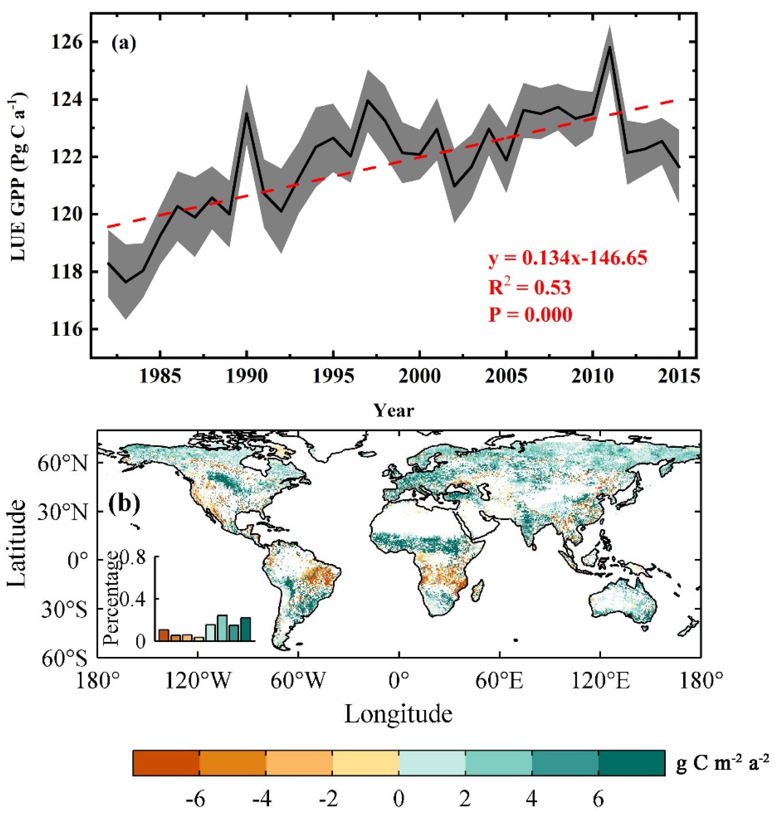
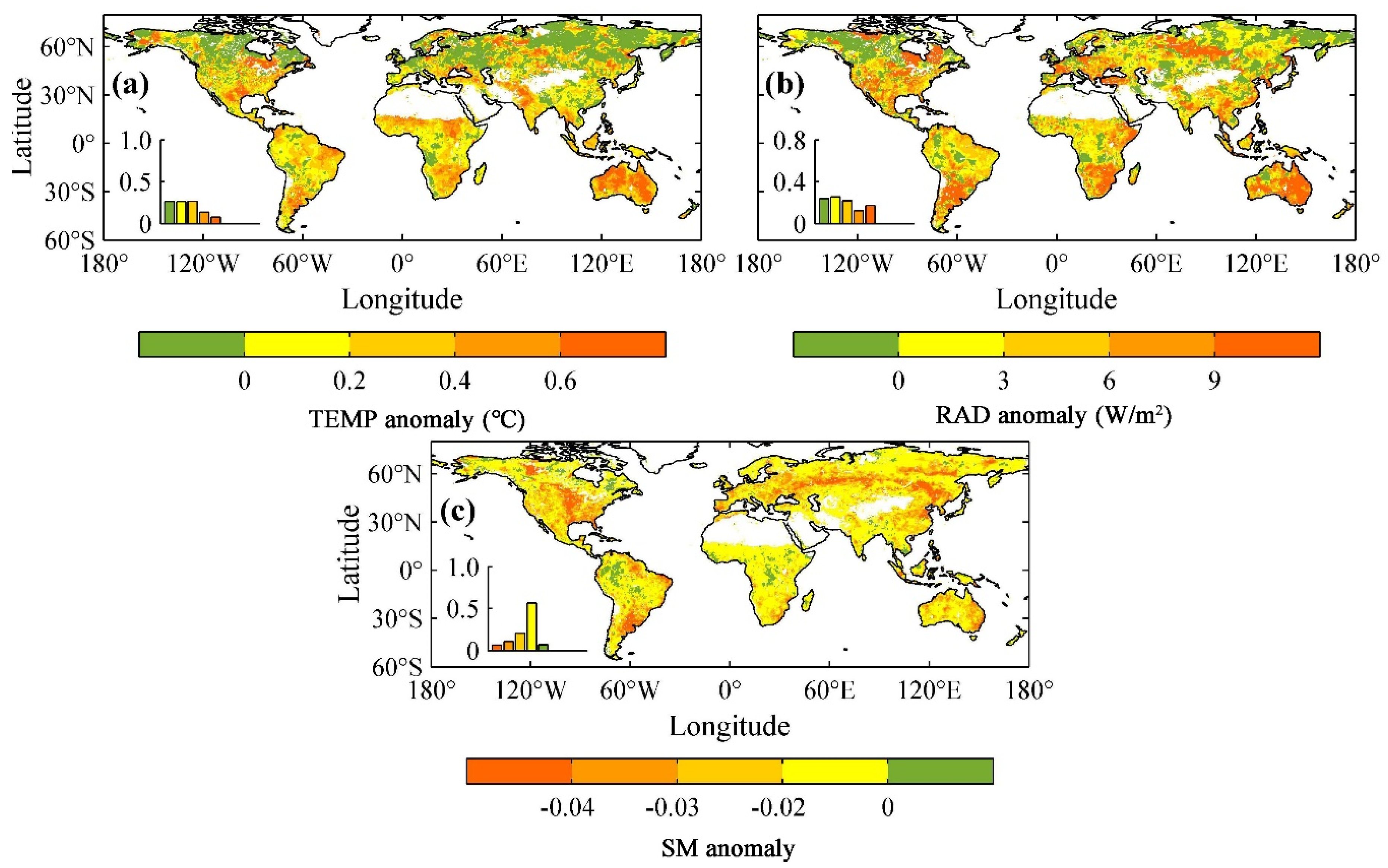
  • Different LUE models have a good fit effect in estimating GPP. The fitting R2 of VPDGLO-SM, VPDMOD-SM, VPDGLO-ETR and VPDMOD-ETR were 0.7739, 0.7399, 0.7427, 0.7459 and 0.7628, respectively. From 1982 to 2015, the global mean annual GPP of terrestrial vegetation continued to increase at an average rate of 0.134 Pg C a −1 (p < 0.001), but its growth rate declined after the mid-1990s. GPP is expected to decrease in 71.91% of the global land vegetation area because of increases in radiation and temperature and decreases in soil moisture during drought periods.
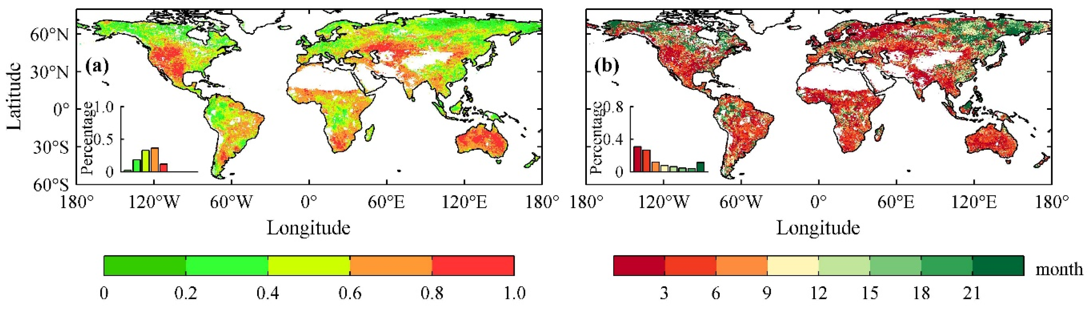
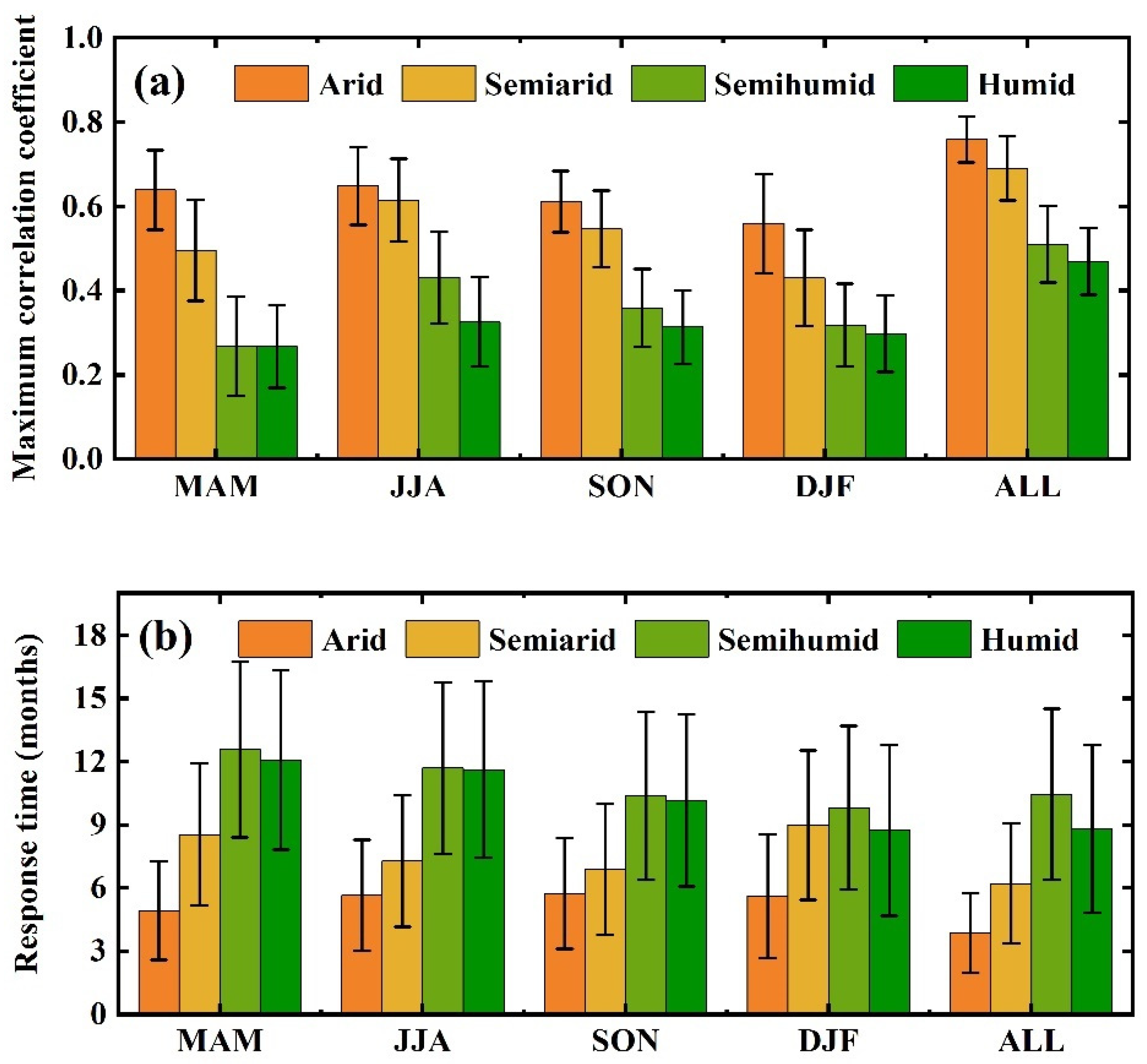
  • Vegetation productivity and water availability are largely correlated positively globally. Further, seasonal changes also affect vegetation productivity’s dependence upon water availability. The correlation coefficient between GPP and SPEI declined from 0.76 to 0.47 as the climatic conditions became gradually humid, indicating that the vegetation productivity in arid and semiarid areas depends more heavily on water availability than that in humid and semi-humid areas. Various land cover types have different adaptation strategies to the increase and loss of water resources, and the productivity of GRA, SAV, and DBF has a higher correlation with water availability.
  • 56.8% of the global terrestrial ecosystems’ response time to water resources is based primarily on short and medium-term time scales (3–6 months). The GPP’s mean response time to SPEI increased from 3.9 to 8.9 months as the climatic conditions became gradually humid, which indicates that the capacity of productivity of vegetation in arid and semiarid areas to withstand long-term water shortages is weaker than that in humid and semi-humid areas. The land cover types that are more relevant to water availability are often accompanied by weak drought resistance, while DNF, OS, EBF and WET have a stronger ability to resist long-term water deficits.
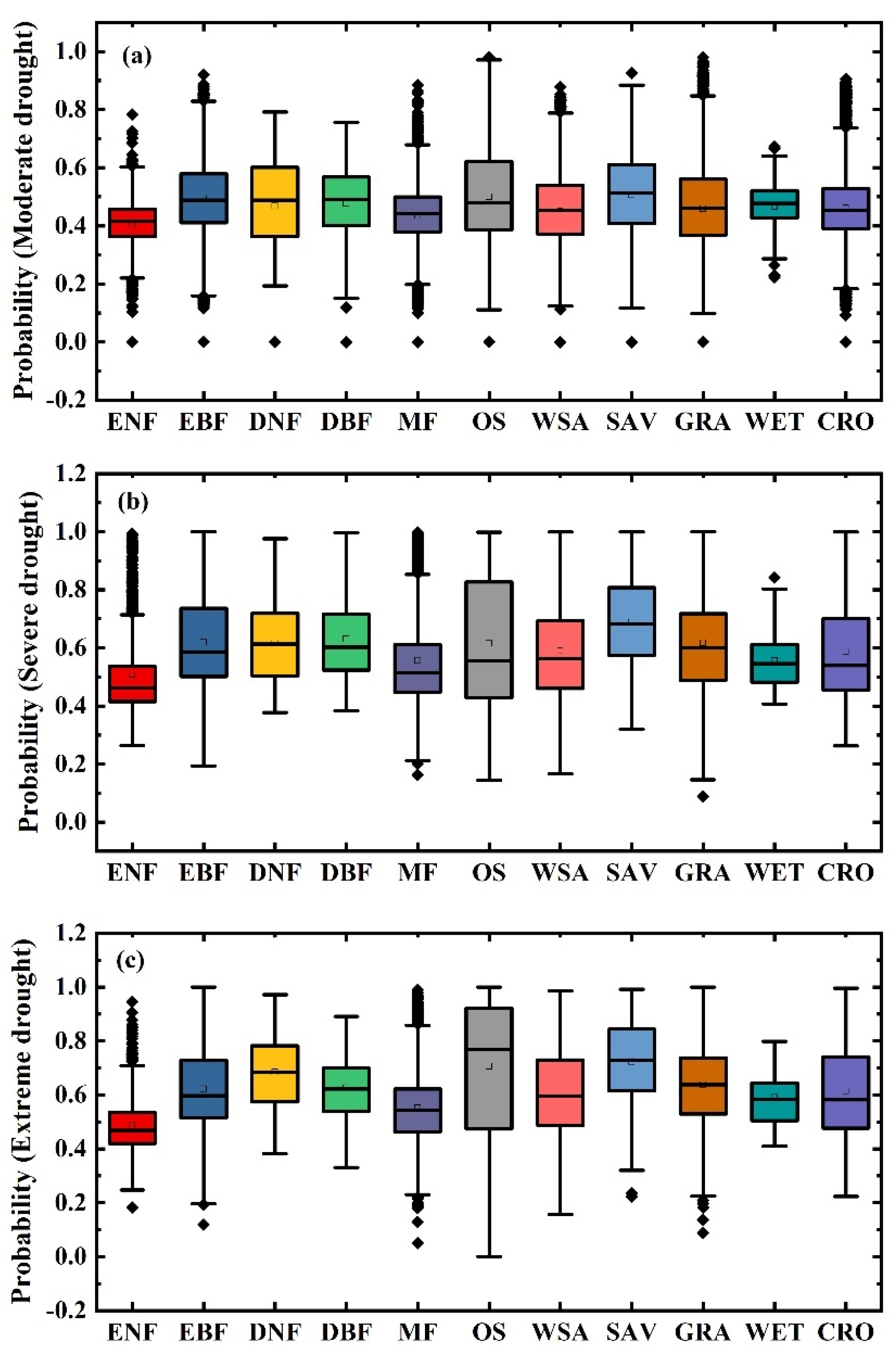
  • Under the scenario of the same level of GPP damage with different drought degrees, as droughts increase in severity, GPP loss probabilities increase as well. Further, under the same drought severity with different levels of GPP damage, drought’s effect on GPP loss probabilities weakens gradually as the GPP damage level increases. Similar patterns were observed in different seasons. Our results showed that arid and semiarid areas have higher conditional probabilities of vegetation productivity losses under different drought scenarios. The productivity loss probability of EBF, DNF, OS, SAV, and GRA show an increasing trend in different seasons, and different land types have different responses to drought in different seasons.

Supplementary Materials

The following are available online at https://www.mdpi.com/article/10.3390/rs13071289/s1, Figure S1: Geographical patterns of the annual ensemble mean LUE model GPPs from 1982 to 2015, Figure S2: The comparison between monthly flux site measurement of GPP and monthly LUE GPP, Figure S3: Geographical patterns of the dependence and response time of vegetation productivity to water availability in different seasons, Figure S4: Spatial distribution of global LUE GPP values at 10th (a), 20th (b), 30th (c) and 40th percentiles (d) during June–August, Figure S5: Spatial distribution of global LUE GPP values at 10th (a), 20th (b), 30th (c) and 40th percentiles (d) during September–November, Figure S6: Spatial distribution of global LUE GPP values at 10th (a), 20th (b), 30th (c) and 40th percentiles (d) during December–February, Figure S7: Conditional probabilities of vegetation productivity losses under different drought scenarios in June-August, Figure S8: Conditional probabilities of vegetation productivity losses under different drought scenarios in September–November, Figure S9: Conditional probabilities of vegetation productivity losses under different drought scenarios in December–February, Figure S10: Conditional probabilities of vegetation productivity losses under different scenarios in various climatic regions in June–August, Figure S11: Conditional probabilities of vegetation productivity losses under different scenarios in various climatic regions in September–November, Figure S12: Conditional probabilities of vegetation productivity losses under different scenarios in various climatic regions in December–February, Figure S13: Conditional probabilities of vegetation productivity losses under different scenarios in different land cover types when the GPP ≤ 40th percentile in June-August, Figure S14: Conditional probabilities of vegetation productivity losses under different scenarios in different land cover types when the GPP ≤ 40th percentile in September–November, Figure S15: Conditional probabilities of vegetation productivity losses under different scenarios in different land cover types when the GPP ≤ 40th percentile in December–February, Table S1: Univariate margin distribution functions, Table S2: Common two-dimensional copula function families.

Author Contributions

Data curation, Y.C.; Supervision, B.F.; Validation, X.W.; Writing—original draft, Y.Z.; Writing—review & editing, X.F. and B.F. All authors have read and agreed to the published version of the manuscript.

Funding

This research was funded by the National Key Research and Development Program of China (2017YFA0604700), National Natural Science Foundation of China (41991233) and Chinese Academy of Sciences (QYZDY-SSW-DQC025 and 2019DC0027).

Institutional Review Board Statement

Not applicable.

Informed Consent Statement

Not applicable.

Data Availability Statement

The data used in the study can be downloaded through the corresponding link provided in Section 2.1.

Conflicts of Interest

The authors declare no conflict of interest.

References

  1. Field, C.B. Climate Change 2014—Impacts, Adaptation and Vulnerability: Regional Aspects; Cambridge University Press: Cambridge, UK, 2014. [Google Scholar]
  2. Cai, W.; Borlace, S.; Lengaigne, M.; Van Rensch, P.; Collins, M.; Vecchi, G.; Timmermann, A.; Santoso, A.; McPhaden, M.J.; Wu, L. Increasing frequency of extreme El Niño events due to greenhouse warming. Nat. Clim. Chang. 2014, 4, 111–116. [Google Scholar] [CrossRef] [Green Version]
  3. Diffenbaugh, N.S.; Giorgi, F. Climate change hotspots in the CMIP5 global climate model ensemble. Clim. Chang. 2012, 114, 813–822. [Google Scholar] [CrossRef] [PubMed] [Green Version]
  4. Beer, C.; Reichstein, M.; Tomelleri, E.; Ciais, P.; Jung, M.; Carvalhais, N.; Rödenbeck, C.; Arain, M.A.; Baldocchi, D.; Bonan, G.B. Terrestrial gross carbon dioxide uptake: Global distribution and covariation with climate. Science 2010, 329, 834–838. [Google Scholar] [CrossRef] [PubMed] [Green Version]
  5. Boyer, J.S. Plant Productivity and Environment. Science 1982, 218, 443–448. [Google Scholar] [CrossRef]
  6. Anav, A.; Friedlingstein, P.; Beer, C.; Ciais, P.; Harper, A.; Jones, C.; Murray-Tortarolo, G.; Papale, D.; Parazoo, N.C.; Peylin, P. Spatiotemporal patterns of terrestrial gross primary production: A review. Rev. Geophys. 2015, 53, 785–818. [Google Scholar] [CrossRef] [Green Version]
  7. Sannigrahi, S.; Zhang, Q.; Joshi, P.K.; Sutton, P.C.; Sen, S. Examining effects of climate change and land use dynamic on biophysical and economic values of ecosystem services of a natural reserve region. J. Clean. Prod. 2020, 257, 120424. [Google Scholar] [CrossRef]
  8. Ryu, Y.; Berry, J.A.; Baldocchi, D.D. What is global photosynthesis? History, uncertainties and opportunities. Remote Sens. Environ. 2019, 223, 95–114. [Google Scholar] [CrossRef]
  9. Zargar, S.M.; Gupta, N.; Nazir, M.; Mahajan, R.; Malik, F.A.; Sofi, N.R.; Shikari, A.B.; Salgotra, R. Impact of drought on photosynthesis: Molecular perspective. Plant Gene 2017, 11, 154–159. [Google Scholar] [CrossRef]
  10. Van Nieuwstadt, M.G.; Sheil, D. Drought, fire and tree survival in a Borneo rain forest, East Kalimantan, Indonesia. J. Ecol. 2005, 93, 191–201. [Google Scholar] [CrossRef]
  11. Reichstein, M.; Ciais, P.; Papale, D.; Valentini, R.; Running, S.; Viovy, N.; Cramer, W.; Granier, A.; OGÉE, J.; Allard, V. Reduction of ecosystem productivity and respiration during the European summer 2003 climate anomaly: A joint flux tower, remote sensing and modelling analysis. Glob. Chang. Biol. 2010, 13, 634–651. [Google Scholar] [CrossRef]
  12. Jentsch, A.; Kreyling, J.; Elmer, M.; Gellesch, E.; Glaser, B.; Grant, K.; Hein, R.; Lara, M.; Mirzae, H.; Nadler, S.E. Climate extremes initiate ecosystem-regulating functions while maintaining productivity. J. Ecol. 2011, 99, 689–702. [Google Scholar] [CrossRef]
  13. Schwalm, C.R.; Williams, C.A.; Schaefer, K.; Baldocchi, D.; Black, T.A.; Goldstein, A.H.; Law, B.E.; Oechel, W.C.; Paw, U.K.T.; Scott, R.L. Reduction in carbon uptake during turn of the century drought in western North America. Nat. Geosci. 2012, 5, 551–556. [Google Scholar] [CrossRef] [Green Version]
  14. Zhang, L.; Xiao, J.; Li, J.; Wang, K.; Lei, L.; Guo, H. The 2010 spring drought reduced primary productivity in southwestern China. Environ. Res. Lett. 2012, 7, 045706. [Google Scholar] [CrossRef] [Green Version]
  15. Stocker, B.D.; Zscheischler, J.; Keenan, T.F.; Prentice, I.C.; Seneviratne, S.I.; Peñuelas, J. Drought impacts on terrestrial primary production underestimated by satellite monitoring. Nat. Geosci. 2019, 12, 264–270. [Google Scholar] [CrossRef]
  16. Craine, J.M.; Ocheltree, T.W.; Nippert, J.B.; Towne, E.G.; Skibbe, A.M.; Kembel, S.W.; Fargione, J.E. Global diversity of drought tolerance and grassland climate-change resilience. Nat. Clim. Chang. 2013, 3, 63–67. [Google Scholar] [CrossRef]
  17. Beguería, S.; Vicente-Serrano, S.M.; Reig, F.; Latorre, B. Standardized precipitation evapotranspiration index (SPEI) revisited: Parameter fitting, evapotranspiration models, tools, datasets and drought monitoring. Int. J. Climatol. 2014, 34, 3001–3023. [Google Scholar] [CrossRef] [Green Version]
  18. Bárdossy, A. Copula-based geostatistical models for groundwater quality parameters. Water Resour. Res. 2006, 42. [Google Scholar] [CrossRef]
  19. Madadgar, S.; AghaKouchak, A.; Farahmand, A.; Davis, S.J. Probabilistic estimates of drought impacts on agricultural production. Geophys. Res. Lett. 2017, 44, 7799–7807. [Google Scholar] [CrossRef]
  20. Fang, W.; Huang, S.; Huang, Q.; Huang, G.; Wang, H.; Leng, G.; Wang, L.; Guo, Y. Probabilistic assessment of remote sensing-based terrestrial vegetation vulnerability to drought stress of the Loess Plateau in China. Remote Sens. Environ. 2019, 232, 111290. [Google Scholar] [CrossRef]
  21. Winkler, A.J.; Myneni, R.B.; Alexandrov, G.A.; Brovkin, V. Earth system models underestimate carbon fixation by plants in the high latitudes. Nat. Commun. 2019, 10, 885. [Google Scholar] [CrossRef]
  22. Yuan, W.; Liu, S.; Zhou, G.; Zhou, G.; Tieszen, L.L.; Baldocchi, D.; Bernhofer, C.; Gholz, H.; Goldstein, A.H.; Goulden, M.L. Deriving a light use efficiency model from eddy covariance flux data for predicting daily gross primary production across biomes. Agric. For. Meteorol. 2007, 143, 189–207. [Google Scholar] [CrossRef] [Green Version]
  23. Bodesheim, P.; Jung, M.; Gans, F.; Mahecha, M.D.; Reichstein, M. Upscaled diurnal cycles of land-atmosphere fluxes: A new global half-hourly data product. Earth Syst. Sci. Data Discuss. 2018, 10, 1327–1365. [Google Scholar] [CrossRef] [Green Version]
  24. Melillo, J.M.; Mcguire, A.D.; Kicklighter, D.W.; Moore, B.; Vorosmarty, C.J.; Schloss, A.L. Global climate change and terrestrial net primary production. Nature 1993, 363, 234–240. [Google Scholar] [CrossRef]
  25. Running, S.W.; Nemani, R.R.; Ann, H.F.; Maosheng, Z.; Matt, R.; Hirofumi, H. A Continuous Satellite-Derived Measure of Global Terrestrial Primary Production. Bioscience 2004, 54, 547–560. [Google Scholar] [CrossRef]
  26. Brecht, M.; Miralles, D.G.; Hans, L.; Robin, V.D.S.; De, J.R.A.M.; Diego, F.-P.; Beck, H.E.; Dorigo, W.A.; Verhoest, N.E.C. GLEAM v3: Satellite-based land evaporation and root-zone soil moisture. Geosci. Model Dev. 2017, 10, 1903–1925. [Google Scholar]
  27. Zhu, Z.; Bi, J.; Pan, Y.; Ganguly, S.; Anav, A.; Xu, L.; Samanta, A.; Piao, S.; Nemani, R.R.; Myneni, R.B. Global data sets of vegetation leaf area index (LAI) 3g and fraction of photosynthetically active radiation (FPAR) 3g derived from global inventory modeling and mapping studies (GIMMS) normalized difference vegetation index (NDVI3g) for the period 1981 to 2011. Remote Sens. 2013, 5, 927–948. [Google Scholar]
  28. Friedl, M.A.; Sulla-Menashe, D.; Tan, B.; Schneider, A.; Ramankutty, N.; Sibley, A.; Huang, X. MODIS Collection 5 global land cover: Algorithm refinements and characterization of new datasets. Remote Sens. Environ. 2010, 114, 168–182. [Google Scholar] [CrossRef]
  29. Vicente-Serrano, S.M.; Beguería, S.; López-Moreno, J.I. A multiscalar drought index sensitive to global warming: The standardized precipitation evapotranspiration index. J. Clim. 2010, 23, 1696–1718. [Google Scholar] [CrossRef] [Green Version]
  30. Feng, S.; Fu, Q. Expansion of global drylands under a warming climate. Atmos. Chem. Phys. 2013, 13, 10081–10094. [Google Scholar] [CrossRef] [Green Version]
  31. Running, S.W.; Thornton, P.E.; Nemani, R.; Glassy, J.M. Global terrestrial gross and net primary productivity from the Earth Observing System. Methods Ecosyst. Sci. 2000, 3, 44–45. [Google Scholar]
  32. Zhang, Y.; Xiao, X.; Wu, X.; Zhou, S.; Zhang, G.; Qin, Y.; Dong, J. A global moderate resolution dataset of gross primary production of vegetation for 2000–2016. Sci. Data 2017, 4, 170165. [Google Scholar] [CrossRef] [PubMed] [Green Version]
  33. Mu, Q.; Heinsch, F.A.; Zhao, M.; Running, S.W. Development of a global evapotranspiration algorithm based on MODIS and global meteorology data. Remote Sens. Environ. 2007, 111, 519–536. [Google Scholar] [CrossRef]
  34. Cramer, W.; Kicklighter, D.; Bondeau, A.; Iii, B.M.; Churkina, G.; Nemry, B.; Ruimy, A.; Schloss, A. Comparing global models of terrestrial net primary productivity (NPP): Overview and key results. Glob. Chang. Biol. 1999, 5, iii–iv. [Google Scholar] [CrossRef]
  35. Potter, C.S.; Randerson, J.T.; Field, C.B.; Matson, P.A.; Klooster, S.A. Terrestrial Ecosystem Production: A Process Model Based on Global Satellite and Surface Data. Glob. Biogeochem. Cycles 1993, 7, 811–841. [Google Scholar] [CrossRef]
  36. Allen, R.; Pereira, L.; Raes, D.; Smith, M.; Allen, R.G.; Pereira, L.S.; Martin, S. Crop Evapotranspiration: Guidelines for Computing Crop Water Requirements; FAO Irrigation and Drainage Paper 56; FAO: Rome, Italy, 1998; p. 56. [Google Scholar]
  37. Task, G.S.D. Global Gridded Surfaces of Selected Soil Characteristics (IGBP-DIS). Ornl Daac. 2000. Available online: https://daac.ornl.gov/cgi-bin/dsviewer.pl?ds_id=569 (accessed on 1 December 2020).
  38. Batjes, N.H. Harmonized soil property values for broad-scale modelling (WISE30sec) with estimates of global soil carbon stocks. Geoderma 2016, 269, 61–68. [Google Scholar] [CrossRef]
  39. Hargreaves, G.H.; Samani, Z.A. Estimating Potential Evapotranspiration. J. Irri. Drain. Div. 1982, 108, 225–230. [Google Scholar] [CrossRef]
  40. Lee, T.; Modarres, R.; Ouarda, T.B. Data-based analysis of bivariate copula tail dependence for drought duration and severity. Hydrol. Process. 2013, 27, 1454–1463. [Google Scholar] [CrossRef]
  41. Zhang, Y.; Feng, X.; Wang, X.; Fu, B. Characterizing drought in terms of changes in the precipitation–runoff relationship: A case study of the Loess Plateau, China. Hydrol. Earth Syst. Sci. 2018, 22, 1749–1766. [Google Scholar] [CrossRef] [Green Version]
  42. Wenwen, C.; Wenping, Y.; Shunlin, L.; Shuguang, L.; Wenjie, D.; Yang, C.; Dan, L.; Haicheng, Z. Large Differences in Terrestrial Vegetation Production Derived from Satellite-Based Light Use Efficiency Models. Remote Sens. 2014, 6, 8945–8965. [Google Scholar]
  43. Zhou, S.; Zhang, Y.; Williams, A.P.; Gentine, P. Projected increases in intensity, frequency, and terrestrial carbon costs of compound drought and aridity events. Sci. Adv. 2019, 5, eaau5740. [Google Scholar] [CrossRef] [Green Version]
  44. Liu, L.; Gudmundsson, L.; Hauser, M.; Qin, D.; Li, S.; Seneviratne, S.I. Soil moisture dominates dryness stress on ecosystem production globally. Nat. Commun. 2020, 11, 4892. [Google Scholar] [CrossRef] [PubMed]
  45. Piao, S.; Zhang, X.; Chen, A.; Liu, Q.; Wu, X. The impacts of climate extremes on the terrestrial carbon cycle: A review. Sci. China Earth Sci. 2019, 62, 1551–1563. [Google Scholar] [CrossRef]
  46. Zhao, M.; Running, S.W. Drought-Induced Reduction in Global Terrestrial Net Primary Production from 2000 through 2009. Science 2010, 329, 940–943. [Google Scholar] [CrossRef] [PubMed] [Green Version]
  47. Xu, H.-J.; Wang, X.-P.; Zhao, C.-Y.; Yang, X.-M. Diverse responses of vegetation growth to meteorological drought across climate zones and land biomes in northern China from 1981 to 2014. Agric. For. Meteorol. 2018, 262, 1–13. [Google Scholar] [CrossRef]
  48. Grossiord, C.; Granier, A.; Ratcliffe, S.; Bouriaud, O.; Bruelheide, H.; Cheko, E.; Forrester, D.I.; Dawud, S.M.; Finér, L.; Pollastrini, M. Tree diversity does not always improve resistance of forest ecosystems to drought. Proc. Natl. Acad. Sci. USA 2014, 111, 14812–14815. [Google Scholar] [CrossRef] [PubMed] [Green Version]
  49. Vicente-Serrano, S.M.; Gouveia, C.; Camarero, J.J.; Beguería, S.; Sanchez-Lorenzo, A. Response of vegetation to drought time-scales across global land biomes. Proc. Natl. Acad. Sci. USA 2012, 110, 52–57. [Google Scholar] [CrossRef] [Green Version]
  50. West, A.G.; Dawson, T.E.; February, E.C.; Midgley, G.F.; Bond, W.J.; Aston, T.L. Diverse functional responses to drought in a Mediterranean-type shrubland in South Africa. New Phytol. 2012, 195, 396–407. [Google Scholar] [CrossRef]
  51. Ivits, E.; Horion, S.; Erhard, M.; Fensholt, R. Assessing European ecosystem stability to drought in the vegetation growing season: Ecosystem stability to drought. Glob. Ecol. Biogeogr. 2016, 25, 1131–1143. [Google Scholar] [CrossRef]
  52. Huang, K.; Yi, C.; Wu, D.; Zhou, T.; Zhao, X.; Blanford, W.J.; Wei, S.; Wu, H.; Ling, D.; Li, Z. Tipping point of a conifer forest ecosystem under severe drought. Environ. Res. Lett. 2015, 10, 024011. [Google Scholar] [CrossRef]
  53. Berdugo, M.; Delgado-Baquerizo, M.; Soliveres, S.; Hernández-Clemente, R.; Zhao, Y.; Gaitán, J.J.; Gross, N.; Saiz, H.; Maire, V.; Lehman, A. Global ecosystem thresholds driven by aridity. Science 2020, 367, 787–790. [Google Scholar] [CrossRef] [Green Version]
Figure 1. The dynamics trend and spatial distribution of the annual ensemble mean light-use efficiency (LUE) model gross primary productivities (GPPs) from 1982 to 2015. (a) Linear trend of annual ensemble mean LUE model GPPs. The shaded areas denote one standard deviation of each corresponding ensemble. (b) Spatial distribution of the linear change rate of GPP during 1982–2015. Only statistically significant trends (p < 0.05) are shown in this figure. The inset shows the corresponding values’ frequency distribution.
Remotesensing 13 01289 g001
Figure 2. Drought frequency and LUE GPP changes’ spatial distribution during the drought period. (a) Geographical pattern of drought frequency from 1982–2015 (based on Standardized Precipitation Evapotranspiration Index (SPEI)–12 month). (b) GPP anomalies during drought period relative to non-drought period.
Remotesensing 13 01289 g002
Figure 3. Geographic distributions of potential climate factors (temperature, radiation and soil moisture) to GPP from 1982 to 2015.
Remotesensing 13 01289 g003
Figure 4. Geographical patterns of vegetation productivity’s dependence upon, and response to, water availability. (a) Spatial distribution of the maximum correlation coefficients recorded between LUE GPP and SPEI in each pixel during 1982–2015. (b) SPEI timescales at which the maximum correlation coefficient between LUE GPP and SPEI was found over the period 1982–2015.
Remotesensing 13 01289 g004
Figure 5. The correlation coefficient (a) and response time (b) of vegetation productivity to water availability in various climatic regions and different seasons. MAM, JJA, SON, DJF, and ALL represent March–May, June–August, September–November, December–February and the entire year, respectively. The error bars indicate ±1 standard error.
Remotesensing 13 01289 g005
Figure 6. The correlation coefficient (a) and response time (b) of vegetation productivity to water availability in different land cover types. ENF, EBF, DNF, DBF, MF, OS, WSA, SAV, GRA, WET and CRO represent evergreen needleleaf forest, evergreen broadleaf forest, deciduous needleleaf forest, deciduous broadleaf forest, mixed forest, open shrublands, woody savannas, savannas, grasslands, wetlands and croplands, respectively. Boxes represent interquartile ranges of the values of 25th and 75th percentiles (Q25, Q75), whiskers cover Q25 − 1.5 × (Q75 − Q25) to Q75 1.5 × (Q75 − Q25), horizontal lines represent the median, black empty squares represent the mean, and black solid diamonds indicate outliers.
Remotesensing 13 01289 g006
Figure 7. Spatial distribution of global LUE GPP values at 10th (a), 20th (b), 30th (c) and 40th percentiles (d) during March–May.
Remotesensing 13 01289 g007
Figure 8. Conditional probabilities of vegetation productivity losses under different drought scenarios in March–May. (ad) represent the conditional probabilities when the GPP ≤ 10th, ≤ 20th, ≤ 30th, and ≤ 40th percentiles in the moderate drought scenario, respectively. (eh) represent the conditional probabilities when the GPP ≤ 10th, ≤ 20th, ≤ 30th, and ≤ 40th percentiles in the severe drought scenario, respectively. (il) represent the conditional probabilities when the GPP ≤ 10th, ≤ 20th, ≤ 30th, and ≤ 40th percentiles in the extreme drought scenario, respectively.
Remotesensing 13 01289 g008
Figure 9. Conditional probabilities of vegetation productivity losses under different scenarios in various climatic regions in March–May. (ac) represent conditional probabilities of vegetation productivity losses under moderate, severe and extreme drought, respectively. GPP loss1, GPP loss2, GPP loss3 and GPP loss4 represent GPP ≤ 10th, ≤ 20th, ≤ 30th, and ≤ 40th percentiles, respectively. The error bars indicate ±1 standard error.
Remotesensing 13 01289 g009
Figure 10. Conditional probabilities of vegetation productivity losses under different drought scenarios in different land cover types when the GPP ≤ 40th percentile in March–May. (ac) represent conditional probabilities of vegetation productivity losses under moderate drought, severe drought and extreme drought, respectively. Boxes represent interquartile ranges of the values of 25th and 75th percentiles (Q25, Q75), whiskers cover Q25 − 1.5 × (Q75 − Q25) to Q75 + 1.5 × (Q75 − Q25), horizontal lines represent the median, black empty squares represent the mean, and black solid diamonds indicate outliers.
Remotesensing 13 01289 g010
Figure 11. Changes in climate factors during the drought period. (ac) show the anomalies of TEMP (Temperature), RAD (Radiation), and SM (soil moisture), respectively, during drought periods compared to those in non-dry periods.
Remotesensing 13 01289 g011
Table 1. Regression statistics for different light-use efficiency models between each land-use type’s measured FLUXNET GPP and LUE GPPs.
Light-Use Efficiency Models
TypeStatisticsVPD onlyVPDGLO-SMVPDMOD-SMVPDGLO-ETRVPDMOD-ETR
DBF (N: 1693)R20.78220.74670.76100.72750.7454
RMSE2.18872.38392.30682.48942.3932
EBF (N: 857)R20.63880.37980.36630.55990.6662
RMSE1.98652.84582.86922.55011.9500
ENF (N: 2968)R20.77060.78330.77330.76710.7590
RMSE1.69901.63991.69191.72781.7697
MF (N: 863)R20.84800.84790.84840.84860.8496
RMSE1.39001.38251.38771.38731.3904
WET (N: 541)R20.68600.58710.62970.59530.6406
RMSE2.07772.50132.31962.46702.2742
CSH/OSH (N: 317)R20.65630.47180.43690.68290.6609
RMSE1.34221.77811.87391.31851.3611
WSA (N: 545)R20.81030.78060.79470.77840.8001
RMSE1.11851.34061.23511.37361.2354
SAV (N: 427)R20.67760.65110.65170.67490.6746
RMSE1.37691.62521.62331.49011.4919
GRA (N: 1767)R20.76670.77270.77300.77540.7763
RMSE1.92141.91751.90881.91371.9012
CRO (N: 1392)R20.52900.46860.50470.45640.4953
RMSE3.5701/
All sites except cropland (N: 9978)R20.77390.73990.74270.74590.7628
RMSE1.80891.98171.96791.97391.8855
Note:The sites are deciduous broadleaf forest (DBF), evergreen broadleaf forest (EBF), evergreen needleleaf forest (ENF), mixed forest (MF), wetlands (WET), closed shrublands/open shrublands (CSH/OSH), woody savanna (WSA), savanna (SAV), grassland (GRA) and cropland (CRO). VPD only, VPDGLO-SM, VPDMOD-SM, VPDGLO-ETR and VPDMOD-ETR stand for the moisture stress algorithms. N represents the total number of data points; R2 is the R2e values of linear regressions with intercept. RMSE represents root mean square error. For each land-use type, the corresponding “best algorithm” is highlighted in bold.
Publisher’s Note: MDPI stays neutral with regard to jurisdictional claims in published maps and institutional affiliations.

