Abstract
The field of human population mapping is constantly evolving, leveraging the increasing availability of high-resolution satellite imagery and the advancements in the field of machine learning. In recent years, the emergence of global built-area datasets that accurately describe the extent, location, and characteristics of human settlements has facilitated the production of new population grids, with improved quality, accuracy, and spatial resolution. In this research, we explore the capabilities of the novel World Settlement Footprint 2019 Imperviousness layer (WSF2019-Imp), as a single proxy in the production of a new high-resolution population distribution dataset for all of Africa—the WSF2019-Population dataset (WSF2019-Pop). Results of a comprehensive qualitative and quantitative assessment indicate that the WSF2019-Imp layer has the potential to overcome the complexities and limitations of top-down binary and multi-layer approaches of large-scale population mapping, by delivering a weighting framework which is spatially consistent and free of applicability restrictions. The increased thematic detail and spatial resolution (~10 m at the Equator) of the WSF2019-Imp layer improve the spatial distribution of populations at local scales, where fully built-up settlement pixels are clearly differentiated from settlement pixels that share a proportion of their area with green spaces, such as parks or gardens. Overall, eighty percent of the African countries reported estimation accuracies with percentage mean absolute errors between ~15% and ~32%, and 50% of the validation units in more than half of the countries reported relative errors below 20%. Here, the remaining lack of information on the vertical dimension and the functional characterisation of the built-up environment are still remaining limitations affecting the quality and accuracy of the final population datasets.
1. Introduction
In the context of global sustainable development, the adoption of the United Nations (UN) Sustainable Development Goals (SDGs) and post-2015 international development agreements ignited a much-needed data revolution, in which countries and institutions all around the world started recognising the fundamental role of geospatial data for policy making [1,2]. Increasingly, high-quality geospatial datasets, in particular those derived from Earth Observation (EO) technologies, are becoming an essential source of information, needed for guiding social, economic and environmental policies at global, regional, national and subnational scales [3,4].
The advantages of employing EO technologies and geospatial datasets to track and monitor sustainable development measures can be summarized as follows. First, compared to ground-based methods, the use of EO technologies, and in particular the use of satellites, allows the production of cost-effective data with a higher frequency over longer periods of time and over larger spatial extents [5,6]. Second, EO technologies enable the collection of near real-time, objective, and independent data for remote and marginalized areas that have previously been ignored [7,8]. Third, when combined with traditional data (e.g., field surveys, census data, demographic and socio-economic statistics), EO data (satellite imagery) supplement and/or enhance the quality of the information by improving its spatial resolution and interpretation capabilities (including better visualization) [3].
In this framework, from a large variety of geospatial datasets that are needed to establish informed sustainable development measures (e.g., data on land-use, land-cover, hazard zones, and climate indicators), some of the most needed spatially explicit datasets are those describing the spatial distribution of the human population [4]. The main reason for this is that accurate knowledge on where and in what density humans live is essential for understanding almost any other type of phenomena, be it social, economic or environmental [9]. This was highlighted in the reviews presented by Kavvada et al. [4], Kuffer et al. [7], and Qui et al. [10], where the authors argue that geospatial data related to human population distributions could potentially be used to directly or indirectly support, implement and monitor more than half of the SDGs (~11 out of 17 SDGs) and a large proportion of their related indicators (~98 of the 231 Indicators). Research in the fields of public security [11], health policy [12,13,14], network and transportation [15], vulnerability and risk assessment [16,17,18], urban growth [19] and mitigation [20] among others, are examples of the many areas where these datasets are needed as inputs to produce reliable information.
Specifically, there are six openly available, large-scale (continental and global) spatially explicit population distribution datasets that are considered “leading datasets for research and decision-making” [21] and which have been produced “to support policies and international agreements in global forums” [22]. These datasets include the High Resolution Settlement layer (HRSL) [23], the WorldPop datasets [24], the Gridded Population of the World (GPWv04) [25], the Global Human Settlement Population datasets (GHS-POP) [26], the Global Rural-Urban Mapping Project (GRUMP) [27] and the LandScan Population datasets (openly available to the educational community) [28,29]. These datasets are available at spatial resolutions of 1, 3 and 30 arcsec (~30 m, ~100 m and ~1 km at the Equator, respectively). Each one of these datasets has been produced using a different “top-down” dasymetric modelling approach [30], consisting in disaggregating administrative unit-based official population counts into grid cells of fixed spatial resolution (e.g., pixels). Disaggregation is normally done through different techniques and using a variety of ancillary geospatial datasets to model, and in some cases restrict, the distribution of population across space. Depending on the selected technique, population datasets can be “lightly modelled” (e.g., areal-weighting, binary- or single-layer-weighted dasymetric redistribution) or “highly modelled” (e.g., multi-layer/intelligent-weighted dasymetric redistribution) (see [31] for more details).
While these products represent the most widely employed top-down large-scale gridded population distribution datasets used today, the field of human population mapping is constantly evolving, leveraging the increasing availability of high-resolution satellite imagery and advancements in the field of machine learning (ML). For the most part, the recent emergence of global (or near-global) built-area datasets that accurately describe the extent, location, and characteristics of human settlements has been exploited in the production of new population grids, resulting in improved quality, accuracy and spatial resolution. Representative examples include recent population distribution datasets that have been produced on the basis of the World Settlement Footprint 2015 products (WSF2015 and WSF2015-Density) [32]; the new WorldPop Sub-Saharan gridded building datasets [33,34,35]; or through the joint analysis of high-resolution binary built-area products [36,37], such as the Global Urban Footprint [38,39], the High Resolution Settlement Layer [23,40] and the Global Human Settlement Layer [41,42], respectively. Here, the particular focus placed on built-area datasets for population modelling arises from the fact that different research has demonstrated that when built-area datasets are used to restrict the distribution of the population, the final products deliver better qualitative and quantitative results in comparison to those models where the datasets are not included [37,43]. In fact, other research has shown that when a given built-area dataset is accurate and coherent enough with population densities, it has the potential to be used as a single proxy for population modelling [43].
In this context, the German Aerospace Center (DLR) is currently working on the development and validation of a new set of global built-area datasets called the WSF2019 and the WSF2019-Impervioussnes (WSF2019-Imp) layers. The first layer is a binary mask outlining the presence of human settlements globally at ~10 m spatial resolution, and the latter is the beta version of a thematic layer estimating the percent impervious surface (PIS) of the pixels marked as settlements in the binary layer. As such, these two datasets represent follow-on products to the WSF2015 and the WSF2015-Density datasets [44,45] however, as different input data were used to produce the WSF2019 datasets, improvements over the 2015 versions can be expected in two main aspects. On the one hand, unlike the WSF2015 layer, which was derived through the joint analysis of Sentinel 1 (S1) radar and Landsat-8 optical imagery (available at ~10 and ~30 m spatial resolution, respectively), the WSF2019 layer is produced by combining S1 data with ~10 m-spatial resolution Sentinel 2 (S2) optical imagery. While still undergoing comprehensive quantitative validation, preliminary results indicate that the increased spatial resolution of the S2 data has allowed for a better identification of building structures compared to the WSF2015 layer, improving the built-up coverage, especially in suburban and rural settings. On the other hand, the calculation of the PIS value, which was previously derived through a multi-temporal analysis of the maximum Normalised Difference Vegetation Index (maxNDVI) extracted from the TimeScan dataset [46], is now derived from the multi-temporal analysis of S2 data. Here, just as before, the employment of higher resolution optical imagery has resulted in remarkable improvements to the thematic accuracy of the layer, delivering a more consistent product compared to the WSF2015-Density layer.
In view of the improvements made over the WSF2015 products, the development of the novel WSF2019 datasets represents a window of opportunity for the production of potentially improved population distribution datasets. Here, the use of the WSF2019-Imp layer for population modelling is of particular interest, as from the many climate-, environmental and geographical factors that correlate with population distributions (e.g., land-cover, topography, distance to waterbodies, distance to roads, access to services, and access to transportation networks), impervious surfaces and built-area datasets have proven to be the strongest predictors of population inhabitation [32,37,47,48]. This means that due to its enhanced thematic characterisation, the WSF2019-Imp layer could potentially be used as single proxy for population modelling, overcoming some of the limitations and complexities of binary and multi-layer approaches [32]. Furthermore, due to its improved spatial resolution (~10 m at the Equator), the final population datasets will likely be more easily integrated with other high-resolution geospatial layers, making them more useful and effective for a broader range of applications compared to existing population grids. Here, previous research has shown that due to their coarse spatial resolution, existing population grids, such as WorldPop and GHS-Pop (~100m and ~1km), perform poorly, especially in application studies carried out at local scales [16].
In this framework, the aim of our research is to explore the capabilities of the novel WSF2019-Imp layer in the production of a new high-resolution large-scale gridded population distribution dataset—the WSF2019-Population (WSF2019-Pop). Using a simple and semi-automatic weighted-dasymetric modelling approach, we incorporate the imperviousness layer with an open archive of subnational census/estimate-based estimates to produce high-resolution population distribution datasets for the African continent. Employing a well-established validation method [31] and leveraging the variably in quality and spatial granularity of the input population data, the main focus of our research is to systematically investigate how accurate and stable the WSF2019-Imp layer is as a single proxy for population modelling. Here, we specifically explore if the WSF2019-Imp layer delivers consistent patterns of accuracy/uncertainty within and among countries, and address the main advantages and limitations of the WSF2019-Imp layer and WSF2019-Pop datasets in support of large-scale population modelling and future research applications, respectively.
2. Materials and Methods
Figure 1 outlines the general process used for the modelling and validation of the WSF2019-Pop dataset for Africa.
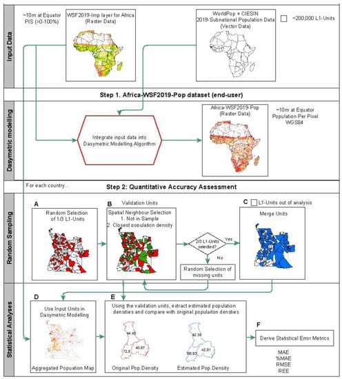
Figure 1.
General workflow for the modelling and validation of the WSF2019-Pop dataset for Africa.
Steps concerning this research include the production of the end-user WSF2019-Pop dataset (Step 1) and the accuracy assessment of the population datasets of each country (Step 2). Input data, namely, the WSF2019-Imp layer for Africa and the 2019 subnational population data, were either made available or downloaded ready-to-use. A detailed description of the main elements (grey labels) of each step are described in more detail in the following sections.
2.1. WSF2019-Imperviousness Layer
Impervious areas are characterised by artificial sealed surfaces that replace natural land-cover or water surfaces. They are normally associated with building structures, streets or sidewalks made out of concrete or stone materials [46]. The WSF2019-Imp layer is part of a series of developments belonging to the WSF portfolio. It was created with the aim of enhancing the semantic and thematic characterization of the WSF2019 settlement layer by describing the PIS within the pixels identified as built-up in the binary layer.
The current processing is based on the same assumption that was used to produce the WSF2015-Density layer [45]. The methodology relies on the fact that a strong inverse relationship exists between impervious surfaces and vegetation, where the higher the vegetation index, the lower the percent of impervious surface within a given built-up pixel. To create the layer, the first step is to compute the maximum temporal NDVI (maxNDVI) from all S2 scenes acquired in 2019, considering only Level 2A bottom of the atmosphere reflectance imagery available globally from December 2017. The maxNDVI is an effective proxy of the presence of vegetation on the ground, where other temporal statistics, such as the mean or median, would not be as effective, since they would be affected—for instance—by the absence of leaves in the cold season. From there, for each of the Köppen–Geiger climate zones, areas associated with impervious surfaces are extracted from OpenStreetMap where these are available, and then rasterized and aggregated at S2 ~10 m spatial resolution. An ensemble of support vector regression (SVR) modules is then employed for properly correlating the resulting training information with the maxNDVI to finally derive the PIS of the pixel marked as settlements in the WSF2019 layer.
Figure 2 provides five different examples of the WSF2019-Imp layer. The first three images (top–bottom) refer to the city of Niamey (Niger), characterized by a hot semi-arid climate; Cairo (Egypt), characterized by a hot desert climate; and the city of Antananarivo (Madagascar), characterized by a subtropical highland climate according to the Köppen Climate classification system, respectively. The last two examples show suburban areas and rural areas in South Africa and Nigeria, and are used to exemplify the local spatial details of the layers in different vegetation cover and urbanised settings. For each of these test sites, additional subsets are compared against Very High Resolution (VHR) satellite imagery.
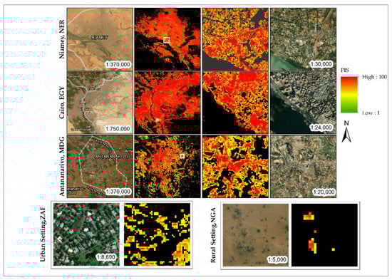
Figure 2.
WSF2019-Imperviouness. Top to bottom: areas of Niamey (Niger), Cairo (Egypt), Antananarivo (Madagascar), and suburban(left) and rural (right) areas in South Africa and Nigeria. Percent impervious surface (PIS) legend from >0% to 100% with country-specific minimum and maximum values. Additional subsets (white boxes) compared against Very High Resolution (VHR) imagery. Black areas: pixels outside the WSF2019 settlement mask.
In this research, the countries of Seychelles and Cape Verde were not included, as consistent S2 data for the selected period were not available when the employed version of the WSF2019-Imp layer was produced.
2.2. Subnational 2019 Population Data
The population estimates for the year 2019 and corresponding subnational administrative unit boundaries (vector data) for all African countries employed in this research were prepared by the Center for International Earth Science Information Network (CIESIN), which, in the context of a cross-organizational collaboration with WorldPop produced population, accounts for the period 2000 to 2020 [49]. For most countries (except Kenya and Malawi), the data were directly downloaded from the open archive of the WorldPop Global Project available at https://doi.org/10.5258/SOTON/WP00650 (accessed on 15 December 2020). The population data for Kenya and Malawi were provided by CIESIN.
All of the population datasets employed here were standardised by CIESIN based upon the methodology described in [50]. The subnational administrative unit boundaries and population counts follow the cartography and official estimates collected in the 2010 round of Population and Housing Censuses, which occurred between 2005 and 2014 (and data from the 2020 round for Kenya and Malawi). From these data, annual exponential growth rates were calculated using two census dates (between circa 2000 and 2010 for most countries) to interpolate and forecast population counts for each subnational administrative unit for the period 2000 to 2020 [49]. The exception is for Kenya, where the cartography [51] and official estimates are from the 2019 census [52], and for Malawi, where the cartography [53] and official estimates are from the 2018 census [54], both of which are part of the 2020 round of Population and Housing Census. This was necessary due to restrictive licenses and significant administrative realignments between the 2010 and 2020 rounds in those countries. For each subnational administrative unit, two types of population estimates are available—census/estimate-based and United Nations-adjusted (UN-adjusted)—with the latter employed for this research following the criterion of existing population datasets, which use UN-adjusted counts as a method of harmonisation [22]. The subnational administrative unit boundaries, referred hereinafter as “L1-units”—according to their original description [49]—represent the highest available administrative unit level specific to each country, and are not comparable within and among countries, in terms of size and administrative level.
Table 1 shows a summary of the input population data. These include the three letter International Organisation for Standardization (ISO) identification code, total population for 2019 adjusted to the UN estimates, the base year of either the census or derived estimation, the number of subnational administrative units and the average spatial resolution (ASR) of the administrative units for each country. The data are presented divided in the five subregions according to the UN geoscheme for Africa [55].

Table 1.
Summary of 2019 UN-adjusted subnational population census/estimate-based data (2019-UNPop) for each African country: 3 letter ISO code, census or estimation year, number of L1-units (L1-U), and the average spatial resolution (ASR). ASR represents the effective resolution of the L1-units in km, calculated as the square root of each country’s total area divided by the number of units.
2.3. Dasymetric Modelling Approach
Gridded population distribution maps for each African country were modelled using a weighted dasymetric mapping approach, where the 2019 UN-adjusted population counts from the input L1-units were redistributed into pixels classified as settlements in the WSF2019-Imlayer (Figure 1, Step 1). For each pixel within an L1-unit, the estimated population count is defined as follows:
According to Equation (1), each pixel within a given input unit is given a proportion of the input unit’s total population , relative to their percent of impervious value . This means, for example, that within a single input unit, the population count of a pixel with a 50% PIS value is twice as high as in a pixel with a 25% PIS value. This modelling technique preserves population input totals, where the sum of population counts of all pixels within an input unit matches the input unit’s original total population.
2.4. Quantitative Accuracy Assessment
In the field of top-down gridded population distribution mapping, and in particular, the area of continental- and global-scale population distribution modelling, validation tasks remain very challenging. In theory, similar to the accuracy assessment of any other RS thematic map, a comprehensive quantitative evaluation of population distribution grids should be based on independent and high-resolution ground-truth data, such as population numbers at the pixel level. However, due to the fact that these types of reference data hardly exist at large scales (e.g., they are only available for some countries) [21,56,57], or when they do exist are difficult to acquire due to privacy protection policies, a “true-validation” of continental and global gridded population distribution datasets is still not possible to implement.
Notwithstanding these limitations, there is, however, an alternative validation method that tests the internal accuracy of large-scale gridded population distribution datasets. In this empirical method, the accuracy of population distribution maps is quantified by computing the differences between the population counts extracted from maps modelled using a coarser (aggregated) level of administrative units (input units) and the actual population counts of the finest administrative units (validation units). The calculated differences at the validation unit level can then be used to derive a variety of statistical error metrics that reflect the relative accuracy, effectiveness, stability and modelling capabilities of the employed disaggregation methods and/or ancillary covariates. Technically speaking, this validation method assumes that the input population data are accurate, and as such, it reports on the quality of the final population grids in terms of “how well and plausibly populations were distributed” [31]. Overall, it is a well-established and accepted validation method, which has been widely employed to investigate the relative accuracies of other large-scale gridded population datasets [15,24,32,37].
Following this premise, in this research, we applied the same validation method to systematically investigate the relative accuracy and mapping capabilities of the WSF2019-Imp layer. The quantitative accuracy assessment presented here comprised two main steps, described as follows.
2.4.1. Random Sampling
To produce the population distribution maps needed for validation, we first generated the aggregated version of the L1-units, following a sampling and merging methodology similar to that employed by Stevens et al. [43]. For each country, we started by randomly selecting one third of the L1-units. For each L1-unit in the sample we then selected a spatial neighbour unit that (1) was not already in the random sample, and (2) had the closest value in population density (Figure 1, Step2-B). This process was performed iteratively until approximately two thirds of the original L1-units were selected. From here, the one third random sample units and the one third selected spatial neighbour units were merged, and their population counts summed to produce coarser units for population modelling (Figure 1, Step 2-C). These coarser units were then used as input units to produce population distribution maps (Equation (1)) (Figure 1, Step 2-D), while the two thirds of sampled L1-units were used for validation (Figure 1, Step2-E). All the remaining unsampled/unmerged L1-units were excluded from the analyses, as their reported differences would have been zero.
The implementation of this aggregation method was deemed necessary, because in each country, the original L1-units represent a mixture of administrative levels, where no attribute is available to identify their administrative levels. Hence, aggregating the L1-units into a common official level, comparable across all countries, was not possible to implement. Consequently, due to the fact that some countries have very large L1-units (Table 1), we selected a merging criterion based on the similarity of population densities, in order to reduce the effect that the size of the input units used for modelling have on the estimation error. Here, research has shown that larger input units tend to present larger estimation errors simply due to their size [32,58]. Finally, we also excluded all the L1-units that reported zero population counts from the sampling process. These units would have generated errors of overestimation of 100%, derived solely from the quality of the input population data, and unrelated to the capabilities of the modelling framework.
The aforementioned sampling method was applied to all African countries, except Comoros. Comoros’ input population data consisted of only three geographically separated polygons representing each of the islands: Grande Comore (Ngazidja), Mohéli (Mwali), and Anjouan (Ndzuani). For the validation of Comoros, the two randomly selected L1-units were merged into a “multi-part” polygon, and their populations were summed. The two L1-units were further used for validation.
2.4.2. Statistical Analyses
From the gridded population distribution maps produced using the coarser input units, population density estimates were extracted for all the sampled L1-units (also referred to as validation units from here on) using the Zonal Statistic tool of ArcGIS (Figure 1, Step 2-E). For each country, the reported differences between the actual population densities and the estimated population densities of the sampled L1-units were then used to derive aggregated error metrics, such as the mean absolute error (MAE) (Equation (3)), the normalised MAE (nMAE or %MAE) (Equation (4)) and the Root Mean Square Error (RMSE) (Equation (5)), and individual error metrics, such as the Relative Estimation Error (REE) (Equation (6)) and the Settlement Size Complexity Index (SSC-Index) (Equation (7)) (Figure 1, Step2-F).
For this research, total population densities were used instead of total population counts to more easily perform comparisons within and among countries with varying population sizes, and with varying numbers and ASR of the sampled L1-units. Statistical analyses were carried out in two ways. First, to perform direct comparisons among countries, the aggregated error metrics were calculated taking into consideration the size/area (km2) of all sampled L1-units that make up each country. This weighting factor removes the bias caused by the differences in size and number of the sampled L1-units among countries, allowing the evaluation of the relative accuracy and modelling stability of the WSF2019-Imp layer at a continental scale. Here, the average population density of each country is then calculated as the conventional population density as follows [59] (Equation (2)):
where , and represent the population, area and density of each individual sampled L1-unit within a country j, respectively. Consequently, the MAE is the average of the sum of absolute differences between the estimated and actual weighted population densities divided by the total area, and the %MAE is the MAE divided by the total population density. Dividing the MAE by the average population density of each country additionally removes the bias caused by the differences in population sizes [60]. The %MAE was chosen over the %RMSE metric, due to the fact that the RMSE is likely to report higher values influenced solely by a larger sample size [61]. Both error metrics measure the average of the absolute errors in the sampled L1-units; however, while MAE weights each error equally, the RMSE gives more weight to larger differences, skewing the errors towards the odd outliers [61]. This quality is useful to check, for example, whether the MAE reported for each country originates from extreme errors or not.
In a broad sense, the area-weighted aggregated metrics assume a proportional distribution of error within each country, allowing us to derive meaningful comparisons among countries. However, as the population density of the individual sampled L1-units varies from unit to unit, so do errors, which are unevenly distributed across space. Therefore, to properly investigate the error distribution within each country, for the second part of the statistical analyses, we calculated the percent REE and the Settlement Size Complexity Index for each sample L1-unit as follows:
The REE is derived by calculating the absolute error between the actual and estimated population density, divided by the actual population density of each unit. Using this metric, each validation was categorised into REE ranges of 20%, following the thresholding criterion employed by [62]. The Settlement Size Complexity Index (SSC-Index) is a metric that was first introduced by Palacios-Lopez et al. [32] to categorise the built-up environment within any given area (polygon boundary) in terms of the size, number, distribution (compacted/spread) and coverage of built-up objects derived from the WSF2015 layer. On the one hand, high SSC-Index values indicate dense built-up environments, where the total area derived from the settlement pixels is almost proportional to the total area of the sample L1-units. Low SSC-Index values, on the other hand, indicate the presence of small and sparse built-up environments, where the coverage of the built-up settlement is proportionally low compared to the total area of the input units. For this research, built-up objects are constructed from the WSF2019-Imp layer, where every object is composed of an 8-neighbourhood connected settlement pixel.
Using a 2D density analysis, we integrated the REE, the population density and the SSC-Index value of each unit to investigate if the REE of a given range was found in validation units with similar characteristics. The 2D density analysis uses contour plots that replace the scatter plot distribution, allowing for better visualisations of clustered data. Contour lines connect the points (validation units) that have the same response value (REE) with regard to two predictors (population density and SSC-Index values) [63].
3. Results
3.1. Africa —WSF2019-Pop Dataset
The end-user WSF2019-Pop dataset for the African continent depicts the residential population for the year 2019 adjusted to the UN national total estimates. The final dataset has a spatial resolution of 0.3 arc-sec (~10 m at the Equator), a WGS84 Geographic Coordinate System projection, and represents the number of people per pixel. Figure 3 shows the WSF2019-Pop dataset that Africa produced on basis of the L1-units of each country. It depicts the areas within the five regions of the continent, using the country boundaries for better visualization. As illustrated, the use of the WSF2019-Imp layer as proxy for population modelling delivers a heterogenous distribution of population guided by the underlying percent of impervious surface value (PIS). The colour scales are country specific.
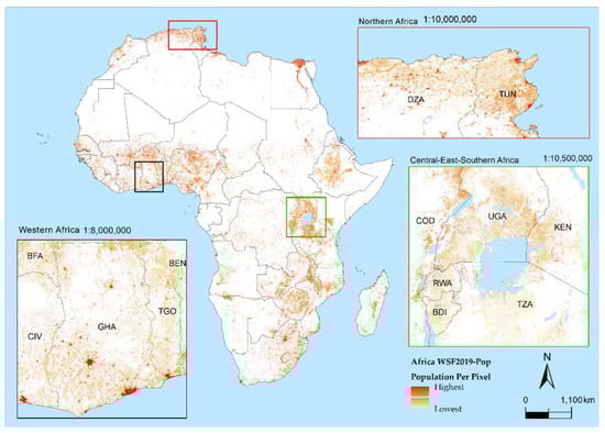
Figure 3.
World Settlement Footprint 2019 Population dataset for Africa (WSF2019-Pop). Colour ranges and values are country specific and represent the estimated population per every ~10 m pixel.
3.2. Quantitative Accuracy Assessment
3.2.1. Random Sampling—Validation Unit Description
For each country, the results of the sampling process described in Section 2.4.1 are presented in Table 2. From an inspection across all African countries, it is possible to observe that the final sample size (n) varies greatly among countries, with values ranging between two sampled L1-units for Comoros (COM), and up to 56,478 sampled L1-units for South Africa (ZAF). Independently of the sample size, results show that for most countries, more that 50% of the total population was covered by the sample, with the exceptions of Congo (COG, 25.62 %), Sao Tome and Prince (STP,48.08 %) and Liberia (LBR, 46.35%). Similarly, for most countries, more than 50% of the total area was covered by the sampled L1-units, with the exceptions of Djibouti (DJI, 20.14%) and Egypt (EGY, 14.12%). Overall, ~70% of Africa’s total population and total area was covered by the random sample.
Table 2.
Summary of the sampled L1-units for each country grouped by region.
For a better visual comparison of each country’s random sample, the distribution of the population density (ppl/km2) and the size (km2) of the sampled L1-units are displayed in the form of violin plots in Figure 4a,b. The shape of the violin plots describes the probability density or frequency of the sampled L1-units within each value range, and the black dots represent the mean value of each metric. From these plots, it is possible to observe, on the one hand, that a large proportion of the sampled L1-units in countries such as Burundi (BDI), Mauritius (MUS), Rwanda (RWA), Uganda (UGA), Egypt (EGY) and South Africa (ZAF) report population densities higher than 100 ppl/km2. A total of 16 countries reported sampled L1-units with population densities higher than 10,000 ppl/km2, with Egypt (EGY) and South Africa (ZAF) among the most representative. On the other hand, some of the lowest population densities are reported in countries such as Algeria (DZA), Western Sahara (ESH), Botswana (BWA), Namibia (NAM), and South Africa (ZAF); here, sampled L1-units show values below 1 ppl/km2.
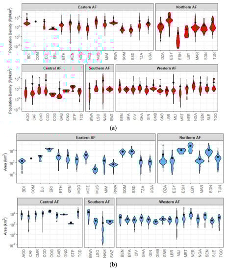
Figure 4.
(a): Violin plots illustrating the distribution of the population density (ppl/km2) of the sample L1-units within each country. Black dot: mean value of the distribution, not to be confused with the average population density of the country. (b): Violin plots illustrating the distribution of the sampled L1-units within each country in terms of their actual size (km2). Black dot: mean value of distribution.
In terms of the size of the sampled L1-units, for most countries, units have variable sizes ranging between 1 km2 and 1000 km2. Countries such as Eritrea (ERI), Somalia (SOM), South Sudan (SSD), Western Sahara (ESH), Libya (LBY), Congo (COG), Gabon (GAB), Equatorial Guinea (GNQ), Chad (TCD), and Botswana (BWA) report units with sizes larger than 10,000 km2, and countries such as Tanzania (TZA), Namibia (NAM), South Africa (ZAF), and Malawi (MLI) report some of the smallest sampled L1-units with areas below 1 km2.
3.2.2. Statistical Analyses
Table 3 summarises the results of the first part of the statistical analyses displaying the average population density (Equation (2)), the MAE (Equation (3)), the %MAE (Equation (4)) and the RMSE (Equation (5)) for each country. A look at the results in terms of the %MAE indicates that the performance of the WSF2019-Imp layer has some minor variabilities across countries. For 80% of the countries located in the upper 10% and lower 90% percentiles (41 countries), the %MAE values ranged from 13.95% to 32.10% with a standard deviation of ±5.32%. Twenty-one of the 41 countries reported %MAE values below or equal to ~20%, ten between ~20% and ~25%, and the last ten between ~25% and ~32%. The lower 10% of the countries reported %MAE values between 6.64% and 12.16%, and the upper 10% reported %MAE values between 35.13% and 72.22%. Within each main region, the lowest and highest %MAE values were reported for Mauritius (MUS,15.51%) and Comoros (COM, 72.22%) in Eastern Africa, Sao Tome and Prince (STP, 12.17%) and Gabon (GAB, 46.57%) in Central Africa, Western Saharan (ESH, 6.64%) and Morocco (MAR, 31.07%) in Northern Africa, South Africa (ZAF,16.72%) and Botswana (BWA, 38.24%) in Southern Africa, and Senegal (SEN, 7.82%) and Mauritania (MRT, 31.66%) in Western Africa, respectively. In terms of the MAE and the RMSE metrics, for all countries, the MAE remained below the average population density value. This behaviour was not the same for the RMSE metric, where for 24 countries, this value exceeded the average population density. According to the distribution of these metrics shown in Figure 5, the difference or ratio between the two metrics is relatively large for countries such as Algeria (DZA), Mauritania (MRT), Mali (MLI), Namibia (NAM), and Angola (AGO). These differences indicate that a large variability exists between the errors of the sampled L1-units within each country.
Table 3.
Statistical metrics for population density.
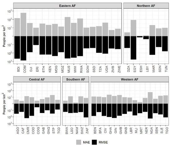
Figure 5.
Bar plots of the distribution of the mean absolute error (MAE) (grey) and Root Mean Square Error (RMSE) (black) of the population density for each country (ISO) within each region.
For the second part of the analyses, we first compared the actual and estimated population density of the validation units of each county. Figure 6 shows these distributions as scatterplots and marginal histograms, depicting the concentration of underestimated (grey) and overestimated (red) validation units. Each plot aggregates the information of all countries within one main African region, so that countries with a small number of units can also be represented. As observed in the tails of the histograms and the scatter of the validation units, there is a tendency of overestimating values below 10 ppl/km2 and underestimating values > ppl/km2. Within the ranges where a larger number of validation units are concentrated, there seems to be a larger tendency towards underestimations; however, the distribution between underestimations and overestimations is somehow proportional across the different population density ranges.
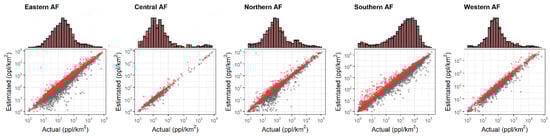
Figure 6.
Scatter plots of estimated population density and actual population density for the validation units of each country within each region. Marginal histograms depict the concentration of underestimations (grey) and overestimations (red). Each panel shows the log population density.
To investigate the general patterns of error distribution within the validation units of each country, Figure 7 shows the percentage of validation units that fall within REE ranges of 20%. From here, it is possible to observe that all countries have at least 20% of their validation units within the >0–20% REE range. For 32 of the 53 countries, this proportion increases to at least 50%, and up to 60% for 16 countries. Sao Tome and Principe (STP), Côte d’Ivoire (CIV), Senegal (SEN), and Togo (TGO) all have at least 75% of the validation within this range, followed by Gambia (GMB) with 100%. For most countries, the second largest proportion of validation units fall within the >20–40% REE range, where at least ~10% but not more than ~30% of the validation units fall within this range. Some exceptions are Zimbabwe (ZWE), Libya (LBY), and Eritrea (ERI), where ~40%, ~50% and ~75% of the validation units fall in this range, respectively. Similarly, the proportion of validation units within the >40–60% range is of at least ~1% for all countries, but no more than ~16%. Here, only Gabon (GAB), Eritrea (ERI), Congo (COG), Djibouti (DJI), and Equatorial Guinea (GNQ) report that ~20% up to ~30% of the validation units fall within this range. From here, 42 of the 53 countries report validation units within REE >60–80%, with 29 of them reporting a proportion of less than 10% of the validation units, from 10% to 20% for 11 countries and 50% for Comoros (COM). Similarly, 35 of the 53 countries report validation units within REE >80–100%, with 30 of them reporting a proportion of less than 10% of the validation units, from 10% to 20% for four countries, and 50% for Comoros (COM). Finally, 38 of the 53 countries report validation units with REE >100%, where 30 of them report a proportion of less than 5%; six from 5% to 7%; and ~10% to ~18% for Botswana (BWA) and Western Sahara (ESH), respectively.
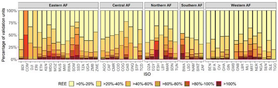
Figure 7.
Stacked bar plots showing the percentage of validation units within each 20% Relative Estimation Error (REE) range.
To explore whether general trends of error distribution are delivered by the WSF2019-Imp layer, for the last part of the statistical analyses, we investigated the relationships among the REE, the population density and the SSC-Index of the validation units. Figure 8 shows the 2D-density plots for the validation units grouped according the different REE ranges. Here, we only present the results for a set of countries where validation units fell within each error range, and where the amount of validation units within each range was enough to produce the contour lines. For comparison purposes, the population density and the SSC-Index values were log-transformed.
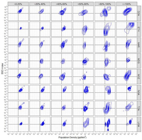
Figure 8.
Two-dimensional-density plots showing the relationship among the population density, the Settlement Size Complexity Index (SSC-Index), and the REE at different ranges of the REE.
From these plots, it is possible to observe that the distribution of the different ranges of REE can be found in the validation units with similar degrees of population density and SSC-Index. There are, however, some general tendencies that can be seen within each error range across most countries, which potentially explain the transitions from one REE range to another. These trends are summarised as follows:
- For all countries, the majority of the validation units with REE between >0% and 40% are located in units with moderately high population densities and moderately high SSC-Index values (top-right quadrant);
- Errors tend to increase as the population density increases and the SSC-Index decreases (shift towards the bottom-right quadrant);
- Large errors (>100%) tend to be located in validation units with extremely high population density and extremely high SSC-Index values;
- Most of the validation units with low population densities and low SSC-Index generally fall within error ranges of REE > 60%.
4. Discussion
4.1. WSF2019-Pop Dataset: Qualitative Assessment
In this research, we presented the production of a new large-scale high-resolution gridded population distribution dataset for the African continent produced on the basis of the WSF2019-Imp layer and openly available subnational census/estimate-based population data. From Figure 1, it is possible to observe that the WSF2019-Imp layer depicts a high likelihood between the estimated PIS values and the underlying built-up environment. High, medium, and low PIS values are proportionally assigned to every 10 × 10 m pixel depending on the density of built-up and green spaces (e.g., parks and gardens) found within them. Here, the specific climate zone of the given region of interest does not seem to generate significant discrepancies in the final calculation of the PIS values, which indicates that the layer is potentially robust, consistent, and comparable across space.
From a practical point of view, the WSF2019-Imp layer provides a weighting framework that is calculated independently of other geospatial layers. This independence provides the final WSF2019-Pop dataset with several advantages over existing binary- and multi-layer products in the following ways. First, as seen from Figure 3, when employed as proxy in a dasymetric modelling approach, the WSF2019-Imp layer produces a heterogenous allocation of population counts that adheres to the variations of PIS values within the L1-units. From a strictly qualitative point of view, this asymmetric distribution of population has shown improvement over the homogenous/uniform distribution delivered by the traditional binary dasymetric approach, revealing more detailed spatial distribution patterns. Previous comparisons presented in Stevens et al. [43], Reed et al. [37], and Palacios-Lopez et al. [32] demonstrated, for example, that binary dasymetric modelling techniques tend to produce visible abrupt changes between census administrative units, whereas weighted approaches (including multi-layer and intelligent dasymetric) smooth these transitions. Second, compared to multi-layer products, another main advantage of the WSF2019-Imp layer is that it allows for the final WSF2019-Pop dataset to be more easily updated and replicated in other areas, without the extensive work that is needed for acquiring multiple geospatial layers of equal quality, extent, spatial resolution, and spatio-temporal coverage [49]. Modelled with a single layer, the final population datasets are potentially more consistent across space in comparison to multi-layer products, in which the quality varies from location to location depending on the number and quality of geospatial datasets available for a given area [29]. In addition to this, as there are no other geospatial datasets involved in the production of the final WSF2019-Pop dataset, the dataset does not suffer from applicability restrictions derived from endogeneity issues [31]. For example, when land-cover data are used to model population datasets, these consequently should not be used for applications focused on understanding correlations between population and land-cover changes.
Notwithstanding these qualitative and practical advantages, as with any other global and regional population distribution dataset, the quality of the final WSF2019-Pop dataset is unavoidably affected by errors and anomalies derived from (1) the completeness and lack of functional characterization of the WSF2019-Imp layer, and (2) the quality of the input population data. Errors derived from the WSF2019-Imp layer include, first of all, a mismatch in the total population counts resulting from the absence of settlements pixels in some populated units. This type of error was identified in three countries: Mauritius (MUS), Morocco (MAR), and South Africa (ZAF). Within each country 8, 49, and 57 populated L1-units reported zero settlement pixels, with a total population sum of 43,931 (3.4%), 337,647 (0.9%), and 230,829 (0.03%), respectively. Through a visual assessment of these countries, we were able to confirm the presence of built-up structures within the reported L1-units. For the most part, the structures were very small and sparse, and were located in environments such as deserted areas or deep valleys. While this underestimation of built-up settlements was also reported for the population distribution datasets produced using the previous WSF2015-Density layer, the amount of validation units with no settlement pixels reported here is considerably less in comparison to the results presented in Palacios-Lopez et al. [32]. For example, in the previous work of Palacios-Lopez et al. [32], where the African countries of Malawi and Côte d’ Ivoire were also analysed, it was found that ~500 units were missing building structures. With the current WSF2019-Imp layer, these two countries reported full coverage, which indicates that the identification of settlement pixels has improved considerably as a result of the integration of S1 and S2 data into the underlying classification framework of the WSF2019 layer.
In the same context, an additional type of error derived from the WSF2019-Imp layer is the allocation of population counts to settlement pixels which are of non-residential use, such as industries, ports, and stadiums. The lack of functional characterization of existing built-up structures is still a persistent limitation that also affects other large-scale gridded population distribution products, such as the HRSL and the GHS-POP datasets. This qualitative limitation has additional quantitative implications, as non-residential, highly impervious surfaces will capture large proportions of the population counts, leading to underestimation in the surrounding settlement pixels. To solve this issue, machine learning methodologies, which are able to classify the residential status of urban buildings from LiDAR data at local scales [64,65], are now applied to large territorial extents using satellite images [66,67]. For example, in the recent work presented by Lloyd et al. [67], the authors combine satellite image-derived building footprint and OSM-label data to classify buildings as residential and non-residential in Democratic Republic of Congo and Nigeria. Their results show that the method classifies buildings with accuracies from 85% to 93% across both countries. Overall, the potential for the large-extent applicability and transferability of this new method will more likely influence the field of large-scale population modelling in the near future.
From the qualitative errors derived from the input population data, the first kind of error is related to the presence of unpopulated units within the population data, where a considerable number of settlement pixels were detected, and where actual populated areas exist. Freire et al. [22] recently addressed this issue, explaining that while the CIESIN census database is the most detailed, complete and coherent database available at global scales, it still presents some anomalies which are derived from the source population statistics (e.g., National Statistic Offices). In this research, ~2099 L1-units were reported as unpopulated, and while some of these units are actually non-enumerated units, some of them still cover large built-up areas according to Freire et al. [22]. In terms of the mapping outcomes, for these L1-units, “NoData” values were assigned to the final settlement pixels resulting in visual inconsistencies in the final population distribution maps. While de-facto no quantitative errors exist in the final population maps in relation to the total input population, the missing counts of these areas can have relevant impacts on further analyses, highlighting the importance of full disclosure on the uncertainties present in the final datasets. To the best of our knowledge, other top-down large-scale gridded population datasets that are based on the CIESIN data currently present the same anomalies.
Finally, the currency and spatial detail of the input population data are other factors that without a doubt affect the quality of the final population distribution maps. As seen from Table 1, for many African countries, the last official population data are from more than 10 years ago, resulting in potentially inaccurate estimates, a low number of administrative units, and outdated administrative boundaries. To be sure, significant improvements have been made in the frequency of population data collection in Africa. Countries such as Burkina Faso, Kenya, Madagascar and Malawi, for example, carried out their last population census between 2018 and 2019, while approximately 80% of the African countries conducted their last census between 2005 and 2015. However, limited financing and poor budgeting strategies for data collection are concurrent issues in many African countries, which result in incomplete or outdated demographic statistics [19]. Under any context, from policy making to scientific research, acquiring up-to-date population data at the highest available resolution should remain the main priority [27].
4.2. WSF2019-Pop Dataset: Quantitative Assessment
To evaluate the relative accuracy, effectiveness, and stability of the WSF2019-Imp layer, for each country, statistical analyses were carried out in two ways: (1) at the country level, where aggregated metrics were computed to allow for cross-country comparisons; (2) at the validation unit level, where individual metrics were computed to establish correlations between the error distribution and the built-up environment. Together, the results presented in Table 3, Figure 7 and Figure 8 show that WSF2019-Imp produces a systematic distribution of error, where estimation accuracies remain relatively consistent among and within countries. At the country level, the population distribution maps of 80% of the countries reported %MAE values between ~15% and ~32%, with a standard deviation of ±~5%. At the validation unit level, for 32 out of 53 countries, at least half of the validation units reported REE values between 0% and 20%, followed by errors of >20–40% and >40–60%. In terms of the error distribution, REE values between >0% and 40% were concentrated in validation units with medium ranges of population density and medium ranges of SSC-Index values, with errors increasing as the SSC-Index decreased and the population density increased. Large estimation errors (>100%) were found in validation units with extremely high population densities and extremely high SSC-Index values.
On that note, whether the presented accuracies can be considered low or high is still a debatable topic [57]. Only a few studies have classified the accuracy results into levels or degrees, but a single threshold of reliability has not yet been established. For example, in the uncertainty quantification of the GRUMP dataset for Poland, Da Costa et al. [62] established that units deviating <20% from the actual population can be considered as “reliable data” and >20% considered as having “medium reliability”. In the accuracy assessment of the GRUMP, GPW, and WorldPop datasets for China presented by Bai el al. [68], the authors established that REE errors <±25% can be considered as “accurately estimated”, between ±25% and ±50% as “under or overestimated”, and from ±50% to >±100% as “greatly under- or overestimated”. Following these criteria, in this research, 25 to 36 countries would be considered as “reliable” or “accurately estimated”, 15 would have “medium reliability”, and two would be found to be poorly reliable. Consequently, within each country and for most countries, the largest proportion of validation units would be “reliable” or “accurately estimated”, while the second largest would have “medium reliability”.
In general, the analyses presented showed that the accuracy of the WSF2019-Imp layer follows the premise established by Stevens et al. [43], who stated that high accuracies in population modelling can be expected when built-up area datasets are proportionally coherent with the population density. The lowest estimation errors in all countries were, for the most part, located in those validation units where the SSC-Index showed a linear correlation with the population density. Notably, as soon as these two factors started to decorrelate, the REE (mainly errors of overestimation) started to increase. Exceptions to this rule applied only to extremely populated units with extremely dense built-up environments, where the largest REE > 100% (mainly errors of underestimation) corresponded to units delineating small cities within the countries.
Overall, the general trends found here are derived from limitations that are consistent across all existing top-down large-scale gridded population datasets. The distribution of error can be explained by four main factors summarised as follows: (1) errors of omission in the identification of built-up settlements in rural settings, which causes the allocation of large population counts into only a few settlement pixels; (2) the potential overestimation of population totals in units with a low number of settlement pixels derived directly from the outdated input population data [23]; (3) the lack of characterisation of the built-up environment (residential/non-residential), which causes the underestimation of population counts in surrounding settlement pixels; and (4) the lack of height and volume (3D) information on the building structures, which causes underestimations, especially in areas with a mix of low- and high-rise buildings.
Nevertheless, there are, however, additional factors that affect the estimation accuracies which are unrelated to the WSF2019-Imp layer. These uncertainties are mainly derived from (a) the nature of the input population data and (b) the sampling process. First, for the majority of countries, there were not enough L1-units to produce significant sample sizes (Table 2). To be able to meet the requirements of a random sampling process that, in parallel, was capable of selecting 2/3 spatially united L1-units as validation units, it was necessary (and unavoidable) to produce sample sizes below 100 units for almost half the countries. Therefore, countries with an already low number of large sampled L1-units, such as Western Sahara (ESH), Senegal (SEN), Gambia (GMB), and Sao Tome and Principe (STP), reported some of the lowest %MAE values, simply due to the small differences in the sizes between the coarser input units used for modelling and the fine units used for validation. This is known as the modifiable areal unit problem (MAUP) [69], which in the context of this research was difficult to avoid without compromising the random sampling process. Second, it goes without saying that different samples for each country will produce different results. This particular limitation was pointed out by Stevens et al. [43] and Sihna et al. [58], who demonstrated that the RMSE and MAE metrics are sensitive to the generated sample in terms of their size and the spatial autocorrelation of the sampled units. Moreover, additional research has also shown that when the sample sizes are very small (4–10 samples), aggregated metrics, such as the RMSE and the MAE, cannot produce robust results [61], highlighting the importance of using individual metrics, such as the REE employed here.
In this context, it is important to understand that the accuracies reported here are constrained to the employed validation method. The final usability and effectiveness of the WSF2019-Pop dataset will also be determined by the accuracy of population estimates extracted in the context of different application scopes. As an example, Figure 9 shows the differences that could be obtained from extracting population counts at very local scales from the WSF2019-Pop dataset and mock-datasets produced using the WSF2019-binary layer. Coastal areas in Morocco and Tanzania illustrate the final population distribution maps produced by each WSF2019 product in medium-to-high urbanised environments. The yellow polygons represent arbitrary areas where population counts were extracted.
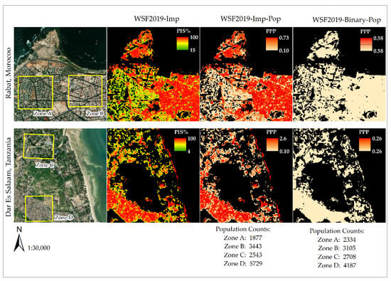
Figure 9.
Final population distribution maps produced using the WSF2019-Imp layer and WSF2019 layer for the coastal areas of Rabat, Morocco, and Dar Es Salaam, Tanzania. From each map, population counts were extracted for Zones A, B, C, and D, respectively. Colour ramps depict values in the current extent.
As seen from Figure 9, extracted population estimates can vary greatly from one dataset to the other. Low impervious areas, such as Zone A and Zone C, allocate less population counts in the WSF2019-Imp layer in comparison to the binary approach. The opposite applies for highly impervious areas, such as Zone B and Zone D, where the binary approach allocates less people per pixel in comparison to the WSF2019-Imp layer. Differences between population datasets range from ~150 to ~1500 people. Depending on the application field where the datasets are employed, the magnitude of these differences can have significant implications, especially in studies where accurate population counts are necessary, such as emergency response or risk assessments.
However, the results presented here are simply used to provide complementary qualitative and quantitative insights into the capabilities of the WSF2019-Imp layer. A complete validation of the results would require real application cases and the availability of reference data. Nonetheless, considering the very local nature of many socio-environmental phenomena [16], it could be expected for the WSF2019-Pop dataset to potentially produce more accurate population estimates compared to currently available binary products (e.g., HRLS and GHS-Pop datasets) and coarse spatial resolution products (e.g., WorldPop and LandScan datasets).
On that note, in this research, we did not include quantitative accuracy comparisons against other available large-scale population grids, as many of the current products do not have datasets representing the year 2019. The closest datasets from the GPWv4, HRSL, and GHS-Pop products, for example, represent population distributions for the years 2015 or 2020. Under these conditions, the temporal disagreement among the different datasets would have introduced a certain level of uncertainty too complex to account for, especially when independent validation data do not exist to verify the results. Here, the lack of validation data is also the reason restricting comparisons with other 2019 population grids, namely, the 2019-WorlPop and 2019-LandScan datasets. Accordingly, comparisons to other built-area datasets (e.g., the 2019-WorldPop building-patterns [34], the 2015-HRSL settlement mask [23], or the 2020 GHSL layer [41]) and modelling methods (e.g., areal-weighting, binary dasymetric, or multi-layer dasymetric) were not included for two main reasons. For the first case, with the validation of the WSF2019-Imp layer in terms of settlement identification still pending, the differences in population estimations between built-area datasets derived from the omission or commission of settlement pixels would not have been possible to address. This means that to properly interpret the differences between the outputs of each built-area dataset, first, we need to know which dataset is more accurate and complete in its own framework. For the second case, comparisons to methods such as areal-weighting and binary-dasymetric were not included, as previous research has already shown that weighted dasymetric mapping is by far more accurate than these two methods [24,32,70]. For the case of multi-layer approaches, comparisons were not included, as the overall objective focuses on exploring the particular advantages or limitations of employing the layer on its own.
5. Conclusions
The present study focused on systematically evaluating how accurate and effective the novel WSF2019-Imperviousness (WSF2019-Imp) layer is in the production of a new large-scale gridded population dataset—the WSF2019-Population dataset (WSF2019-Pop). Employed as a single proxy in a dasymetric mapping approach, the WSF2019-Imp layer was used in combination with an open archive of census/estimate-based population data to construct population datasets for each African country.
Results of our qualitative and quantitative assessment indicate that the main advantages of the WSF2019-Imp layer as a proxy for large-scale population modelling, are derived from its robustness, spatial consistency, independent weighting framework, and improved spatial resolution. These characteristics allow the layer to produce spatially detailed population datasets that could potentially be more accurate than binary-derived products, on the one hand, and that could potentially overcome the local qualitative variations, applicability restrictions, and production complexities of multi-layer-derived products, on the other. The results of our statistical analyses additionally confirm that the WSF2019-Imp layer is capable of producing a systematic distribution of error that remains stable independently of the quality and spatial granularity of the input population data. Overall, the WSF2019-Imp layer reported %MAE values between ~15% and ~32% for close to 80% and REE below 20% for up to 50% of the validation units of most countries. Following the pre-established classification criterion, these error ranges indicate that the WSF2019-Imp layer produces, for the most part, “accurately estimated” population datasets. Notwithstanding these promising results, there are, however, some limitations that still need to be addressed, as high errors of underestimation and overestimation are still present in the final WSF2019-Pop dataset. In particular, the omission of settlement pixels in rural settings and the lack of information on the use and height of the building structures are factors that currently affect the quality and accuracy of the final population datasets. In this context, it is expected that with the upcoming validation of the WSF2019 products, these remaining uncertainties can be assessed, allowing a focus on further technical improvements to the WSF2019-Pop dataset. Considering this, future research will also include quantitative comparisons with other built-area datasets and population grids, and the integration of other geospatial layers into the modelling framework, such as the newly developed Global Urban Footprint 3D dataset [71]. Furthermore, as the semi-automatic methods presented here are completely transferable, future research will also focus on expanding the accuracy assessment of the WSF2019-Pop dataset to other countries. Within this outlook, the WSF2019-Pop dataset will also be evaluated in the framework of different application fields, especially those related to risk assessment and emergency response. Here, additional comparisons with other population grids will be performed to assess their accuracy, usability, and limitations.
To conclude, the WSF2019-Population dataset developed in this research represents an important contribution to the field of large-scale gridded population mapping, helping to improve and enhance the spatial granularity and local detail of census population data needed for a wide range of research and governmental applications. In the context of risk assessment, the WSF2019-Pop dataset is currently used by the World Bank to identify all localities on the African continent with an estimated population of >10,000 inhabitants. Additionally, the population at risk with respect to urban hazard zones, such as seismic, landslides, flooding, and storm surge, is determined based on a combination of the WSF2019-Pop layer and risk data, such as those provided by the Think Hazard! datasets [72]. Open and free provision of the WSF2019-Pop dataset is foreseen through the Urban Thematic Exploitation Platform (https://urban-tep.eu (accessed on 15 December 2020)) and the Earth Observation Center Geoservice (https://geoservice.dlr.de (accessed on 15 December 2020)).
Author Contributions
Conceptualization, D.P.-L., M.M., P.R. and T.E.; methodology, D.P.-L., A.S. and A.J.T.; software, J.Z. and D.P.-L.; validation, D.P.-L.; formal analysis, D.P.-L.; investigation, D.P-L.; resources, A.S. and K.M.; data curation, D.P.-L., M.M. and K.M.; writing—original draft preparation, D.P.-L.; writing—review and editing, F.B., T.E., M.M., K.M., A.S. and A.J.T.; visualization, D.P.-L.; supervision, P.R., T.E., A.J.T. and S.D.; funding acquisition, T.E. and S.D. All authors have read and agreed to the published version of the manuscript.
Funding
This research received no external funding.
Data Availability Statement
The 2019 UN-adjusted population data presented in this study are publicly available datasets. This data can be found here: https://doi.org/10.5258/SOTON/WP00650 (accessed on 15 December 2020). The WSF2019-Pop dataset is not publicly available due to pending data validation and related publication of the WSF2019 datasets. Open and free provision is foreseen in the following online platforms: https://urban-tep.eu (accessed on 15 December 2020) and https://geoservice.dlr.de (accessed on 15 December 2020).
Acknowledgments
The authors would like to thank the CIESIN and WorldPop organisations for the administrative boundaries and census/estimate-base population data for the year 2019 for the whole of Africa.
Conflicts of Interest
The authors declare no conflict of interest.
References
- United Nations. The future we want. In Proceedings of the Rio+20 United Nations Conference on Sustainable Development, Rio de Janeiro, Brazil, 20–22 June 2012. [Google Scholar]
- United Nations. Strengthening the Demographic Evidence Base for the Post-2015 Development Agenda. A Concise Report; United Nations, Department of Economic and Social Affairs, Population Division: New York, NY, USA, 2016. [Google Scholar]
- Anderson, K.; Ryan, B.; Sonntag, W.; Kavvada, A.; Friedl, L. Earth observation in service of the 2030 Agenda for Sustainable Development. Geo-Spat. Inf. Sci. 2017, 20, 77–96. [Google Scholar] [CrossRef]
- Kavvada, A.; Metternicht, G.; Kerblat, F.; Mudau, N.; Haldorson, M.; Laldaparsad, S.; Friedl, L.; Held, A.; Chuvieco, E. Towards delivering on the sustainable development goals using earth observations. Remote Sens. Environ. 2020, 247, 111930. [Google Scholar] [CrossRef]
- Andries, A.; Morse, S.; Murphy, R.; Lynch, J.; Woolliams, E.; Fonweban, J. Translation of Earth observation data into sustainable development indicators: An analytical framework. Sustain. Dev. 2019, 27, 366–376. [Google Scholar] [CrossRef]
- Craglia, M.; Pogorzelska, K. The Economic Value of Digital Earth. In Manual of Digital Earth; Guo, H., Goodchild, M.F., Annoni, A., Eds.; Springer: Singapore, 2019; pp. 623–643. [Google Scholar]
- Kuffer, M.; Thomson, D.R.; Boo, G.; Mahabir, R.; Grippa, T.; Van Huysse, S.; Engstrom, R.; Ndugwa, R.; Makau, J.; Darin, E.; et al. The Role of Earth Observation in an Integrated Deprived Area Mapping “System” for Low-to-Middle Income Countries. Remote Sens. 2020, 12, 982. [Google Scholar] [CrossRef]
- Ansari, R.A.; Buddhiraju, K.M. Textural segmentation of remotely sensed images using multiresolution analysis for slum area identification. Eur. J. Remote Sens. 2019, 52, 74–88. [Google Scholar] [CrossRef]
- Aguirre, M.S. Sustainable development: Why the focus on population? Int. J. Soc. Econ. 2002, 29, 923–945. [Google Scholar] [CrossRef]
- Qiu, Y.; Zhao, X.; Fan, D.; Li, S. Geospatial Disaggregation of Population Data in Supporting SDG Assessments: A Case Study from Deqing County, China. ISPRS Int. J. Geo-Inf. 2019, 8, 356. [Google Scholar] [CrossRef]
- Galway, L.; Bell, N.; Sae, A.S.; Hagopian, A.; Burnham, G.; Flaxman, A.; Weiss, W.M.; Rajaratnam, J.; Takaro, T.K. A two-stage cluster sampling method using gridded population data, a GIS, and Google EarthTM imagery in a population-based mortality survey in Iraq. Int. J. Health Geogr. 2012, 11, 12. [Google Scholar] [CrossRef] [PubMed]
- Fries, B.; Smith, D.L.; Wu, S.; Dolgert, A.J.; Guerra, C.A.; Hay, S.I.; García, G.A.; Smith, J.M.; Oyono, J.N.M.; Donfack, O.T. Measuring the accuracy of gridded human population density surfaces: A case study in Bioko Island, Equatorial Guinea. bioRxiv 2020. [Google Scholar] [CrossRef]
- Hay, S.I.; Noor, A.M.; Nelson, A.; Tatem, A.J. The accuracy of human population maps for public health application. Trop. Med. Int. Health 2005, 10, 1073–1086. [Google Scholar] [CrossRef] [PubMed]
- Tatem, A.J.; Campiz, N.; Gething, P.W.; Snow, R.W.; Linard, C. The effects of spatial population dataset choice on estimates of population at risk of disease. Popul. Health Metr. 2011, 9, 4. [Google Scholar] [CrossRef] [PubMed]
- Linard, C.; Gilbert, M.; Snow, R.W.; Noor, A.M.; Tatem, A.J. Population Distribution, Settlement Patterns and Accessibility across Africa in 2010. PLoS ONE 2012, 7, e31743. [Google Scholar] [CrossRef] [PubMed]
- Smith, A.; Bates, P.D.; Wing, O.; Sampson, C.; Quinn, N.; Neal, J. New estimates of flood exposure in developing countries using high-resolution population data. Nat. Commun. 2019, 10, 1814. [Google Scholar] [CrossRef]
- Calka, B.; Da Costa, J.N.; Bielecka, E. Fine scale population density data and its application in risk assessment. Geomat. Nat. Hazards Risk 2017, 8, 1440–1455. [Google Scholar] [CrossRef]
- Zischg, A.P.; Bermúdez, M. Mapping the Sensitivity of Population Exposure to Changes in Flood Magnitude: Prospective Application from Local to Global Scale. Front. Earth Sci. 2020, 8, 390. [Google Scholar] [CrossRef]
- Tuholske, C.; Caylor, K.; Evans, T.; Avery, R. Variability in urban population distributions across Africa. Environ. Res. Lett. 2019, 14, 085009. [Google Scholar] [CrossRef]
- Chen, Y.; Guo, F.; Wang, J.; Cai, W.; Wang, C.; Wang, K. Provincial and gridded population projection for China under shared socioeconomic pathways from 2010 to 2100. Sci. Data 2020, 7, 83. [Google Scholar] [CrossRef]
- Bustos, M.F.A.; Hall, O.; Niedomysl, T.; Ernstson, U. A pixel level evaluation of five multitemporal global gridded population datasets: A case study in Sweden, 1990–2015. Popul. Environ. 2020, 42, 255–277. [Google Scholar] [CrossRef]
- Freire, S.; Schiavina, M.; Florczyk, A.J.; MacManus, K.; Pesaresi, M.; Corbane, C.; Borkovska, O.; Mills, J.; Pistolesi, L.; Squires, J.; et al. Enhanced data and methods for improving open and free global population grids: Putting ‘leaving no one behind’ into practice. Int. J. Digit. Earth 2020, 13, 61–77. [Google Scholar] [CrossRef]
- Tiecke, T.G.; Liu, X.; Zhang, A.; Gros, A.; Li, N.; Yetman, G.; Kilic, T.; Murray, S.; Blankespoor, B.; Prydz, E.B. Mapping the World Population One Building at a Time. arXiv 2017, arXiv:1712.05839. [Google Scholar]
- Stevens, F.F.; Gaughan, A.A.; Linard, C.; Tatem, A.A. Disaggregating Census Data for Population Mapping Using Random Forests with Remotely-Sensed and Ancillary Data. PLoS ONE 2015, 10, e0107042. [Google Scholar] [CrossRef]
- Doxsey-Whitfield, E.; MacManus, K.; Adamo, S.B.; Pistolesi, L.; Squires, J.; Borkovska, O.; Baptista, S.R. Taking Advantage of the Improved Availability of Census Data: A First Look at the Gridded Population of the World, Version 4. Pap. Appl. Geogr. 2015, 1, 226–234. [Google Scholar] [CrossRef]
- Freire, S.; Doxsey-Whitfield, E.; MacManus, K.; Mills, J.; Pesaresi, M. Development of new open and free multi-temporal global population grids at 250 m resolution. In Proceedings of the 19th AGILE Conference on Geographic Information Science, Helsinki, Finland, 14–17 June 2016. [Google Scholar]
- Balk, D.; Deichmann, U.; Yetman, G.; Pozzi, F.; Hay, S.; Nelson, A. Determining Global Population Distribution: Methods, Applications and Data. Adv. Parasitol. 2006, 62, 119–156. [Google Scholar] [CrossRef] [PubMed]
- Bhaduri, B.; Bright, E.; Coleman, P.; Urban, M.L. LandScan USA: A high-resolution geospatial and temporal modeling approach for population distribution and dynamics. GeoJournal 2007, 69, 103–117. [Google Scholar] [CrossRef]
- Dobson, J.E.; Bright, E.A.; Coleman, P.R.; Durfee, R.C.; Worley, B.A. LandScan: A global population database for estimating populations at risk. Photogramm. Eng. Remote Sens. 2000, 66, 849–857. [Google Scholar] [CrossRef]
- Mennis, J. Generating surface models of population using dasymetric mapping. Prof. Geogr. 2003, 55, 31–42. [Google Scholar]
- Leyk, S.; Gaughan, A.E.; Adamo, S.B.; De Sherbinin, A.; Balk, D.; Freire, S.; Rose, A.; Stevens, F.R.; Blankespoor, B.; Frye, C.; et al. The spatial allocation of population: A review of large-scale gridded population data products and their fitness for use. Earth Syst. Sci. Data 2019, 11, 1385–1409. [Google Scholar] [CrossRef]
- Palacios-Lopez, D.; Bachofer, F.; Esch, T.; Heldens, W.; Hirner, A.; Marconcini, M.; Sorichetta, A.; Zeidler, J.; Kuenzer, C.; Dech, S.; et al. New Perspectives for Mapping Global Population Distribution Using World Settlement Footprint Products. Sustain. J. Rec. 2019, 11, 6056. [Google Scholar] [CrossRef]
- Maxar Technologies. Building Footprints. Available online: https://www.maxar.com/products/building-footprints (accessed on 6 January 2021).
- WorldPop. Gridded Maps of building patterns through sub-Saharan Africa (Version 1). 2020. Available online: https://doi.org//10.5258/SOTON/WP00677 (accessed on 15 December 2020).
- Population Counts/Contrain Individual Countries 2020 (100 m). Available online: https://www.worldpop.org/geodata/listing?id=78 (accessed on 1 January 2020).
- Nieves, J.J.; Sorichetta, A.; Linard, C.; Bondarenko, M.; Steele, J.E.; Stevens, F.R.; Gaughan, A.E.; Carioli, A.; Clarke, D.J.; Esch, T.; et al. Annually modelling built-settlements between remotely-sensed observations using relative changes in subnational populations and lights at night. Comput. Environ. Urban Syst. 2020, 80, 101444. [Google Scholar] [CrossRef] [PubMed]
- Reed, F.J.; Gaughan, A.E.; Stevens, F.R.; Yetman, G.; Sorichetta, A.; Tatem, A.J. Gridded Population Maps Informed by Different Built Settlement Products. Data 2018, 3, 33. [Google Scholar] [CrossRef]
- Esch, T.; Heldens, W.; Hirner, A.; Keil, M.; Marconcini, M.; Roth, A.; Zeidler, J.; Dech, S.; Strano, E. Breaking new ground in mapping human settlements from space—The Global Urban Footprint. ISPRS J. Photogramm. Remote Sens. 2017, 134, 30–42. [Google Scholar] [CrossRef]
- Esch, T.; Bachofer, F.; Heldens, W.; Hirner, A.; Marconcini, M.; Palacios-Lopez, D.; Roth, A.; Üreyen, S.; Zeidler, J.; Dech, S.; et al. Where We Live—A Summary of the Achievements and Planned Evolution of the Global Urban Footprint. Remote Sens. 2018, 10, 895. [Google Scholar] [CrossRef]
- Connecting the World with Better Maps. Available online: https://engineering.fb.com/2016/02/21/core-data/connecting-the-world-with-better-maps/ (accessed on 15 October 2020).
- Pesaresi, M.; Ehrlich, D.; Ferri, S.; Florczyk, A.; Freire, S.; Halkia, M.; Julea, A.; Kemper, T.; Soille, P.; Syrris, V. Operating procedure for the production of the Global Human Settlement Layer from Landsat data of the epochs 1975, 1990, 2000, and 2014. Publ. Off. Eur. Union 2016. [Google Scholar] [CrossRef]
- Pesaresi, M.; Huadong, G.; Blaes, X.; Ehrlich, D.; Ferri, S.; Gueguen, L.; Halkia, M.; Kauffmann, M.; Kemper, T.; Luigi, Z.; et al. A Global Human Settlement Layer from Optical HR/VHR RS Data: Concept and First Results. IEEE J. Sel. Top. Appl. Earth Obs. Remote Sens. 2013, 6, 2102–2131. [Google Scholar] [CrossRef]
- Stevens, F.R.; Gaughan, A.E.; Nieves, J.J.; King, A.; Sorichetta, A.; Linard, C.; Tatem, A.J. Comparisons of two global built area land cover datasets in methods to disaggregate human population in eleven countries from the global South. Int. J. Digit. Earth 2019, 13, 78–100. [Google Scholar] [CrossRef]
- Marconcini, M.; Metz-Marconcini, A.; Üreyen, S.; Palacios-Lopez, D.; Hanke, W.; Bachofer, F.; Zeidler, J.; Esch, T.; Gorelick, N.; Kakarla, A. Outlining where humans live—The World Settlement Footprint 2015. Sci. Data 2019. [Google Scholar] [CrossRef]
- Marconcini, M.; Metz-Marconcini, A.; Zeidler, J.; Esch, T. Urban Monitoring in Support of Sustainable Cities; 2015 Joint Urban Remote Sensisn Event (JURSE): Piscataway, NJ, USA, 2015. [Google Scholar]
- Azar, D.; Graesser, J.; Engstrom, R.; Comenetz, J.; Leddy, R.M., Jr.; Schechtman, N.G.; Andrews, T. Spatial refinement of census population distribution using remotely sensed estimates of impervious surfaces in Haiti. Int. J. Remote Sens. 2010, 31, 5635–5655. [Google Scholar] [CrossRef]
- Nieves, J.J.; Stevens, F.R.; Gaughan, A.E.; Linard, C.; Sorichetta, A.; Hornby, G.; Patel, N.N.; Tatem, A.J. Examining the correlates and drivers of human population distributions across low- and middle-income countries. J. R. Soc. Interface 2017, 14, 20170401. [Google Scholar] [CrossRef]
- Lu, D.; Weng, Q.; Li, G. Residential population estimation using a remote sensing derived impervious surface approach. Int. J. Remote Sens. 2006, 27, 3553–3570. [Google Scholar] [CrossRef]
- Lloyd, C.T.; Chamberlain, H.; Kerr, D.; Yetman, G.; Pistolesi, L.; Stevens, F.R.; Gaughan, A.E.; Nieves, J.J.; Hornby, G.; MacManus, K.; et al. Global spatio-temporally harmonised datasets for producing high-resolution gridded population distribution datasets. Big Earth Data 2019, 3, 108–139. [Google Scholar] [CrossRef] [PubMed]
- Center of International Earth Science Information Network (CIESIN). Documentation for the Gridded Population of the World (GPWv4.0) (Version 4); CIESIN: Palisades, NY, USA, 2015. [Google Scholar] [CrossRef]
- Kenya National Bureau of Statistics. Sub-County Boundaries; Office of General Director: Nairobi, Kenya, 2020. [Google Scholar]
- Kenya National Bureau of Statistics. Population and Housing Census 2019: Table: Census Volume 1 Question 1 Population by County and Subcounty. 2019. Available online: https://www.knbs.or.ke/?wpdmpro=2019-kenya-population-and-housing-census-volume-i-population-by-county-and-sub-county (accessed on 15 November 2020).
- Humanitarian Data Exchange. Malawi Traditional Authority. 2018. Available online: https://data.humdata.org/dataset/2018_malawi_ta_dataset-updated-admin3 (accessed on 15 November 2020).
- Malawi National Statistical Office. Population and Housing Census 2018, Series A Population Table (Series A). 2018. Available online: http://www.nsomalawi.mw/images/stories/data_on_line/demography/census_2018/2018%20MPHC%20Published%20Tables/Series%20A.%20Population%20Tables.xlsx (accessed on 15 November 2020).
- United Nations Statistics Division.Standard Country or Area Codes for Statistical Use (M49). 2020. Available online: https://unstats.un.org/unsd/methodology/m49/ (accessed on 23 September 2020).
- Calka, B.; Bielecka, E. GHS-POP Accuracy Assessment: Poland and Portugal Case Study. Remote Sens. 2020, 12, 1105. [Google Scholar] [CrossRef]
- Calka, B.; Bielecka, E. Reliability Analysis of LandScan Gridded Population Data. The Case Study of Poland. ISPRS Int. J. Geo-Inf. 2019, 8, 222. [Google Scholar] [CrossRef]
- Sinha, P.; Gaughan, A.E.; Stevens, F.R.; Nieves, J.J.; Sorichetta, A.; Tatem, A.J. Assessing the spatial sensitivity of a random forest model: Application in gridded population modeling. Comput. Environ. Urban Syst. 2019, 75, 132–145. [Google Scholar] [CrossRef]
- Ottensmann, J.R.M. On Population-Weighted Density. SSRN Electron. J. 2018. [Google Scholar] [CrossRef]
- Vandeput, N. Forecasting KPIs: RMSE, MAE, MAPE & Bias. Available online: https://towardsdatascience.com/forecast-kpi-rmse-mae-mape-bias-cdc5703d242d (accessed on 19 October 2020).
- Chai, T.; Draxler, R.R. Root mean square error (RMSE) or mean absolute error (MAE)?—Arguments against avoiding RMSE in the literature. Geosci. Model Dev. 2014, 7, 1247–1250. [Google Scholar] [CrossRef]
- Da Costa, J.N.; Bielecka, E.; Calka, B. Uncertainty Quantification of the Global Rural-Urban Mapping Project over Polish Census Data. In Proceedings of the “Environmental Engineering” 10th International Conference, Vilnius, Lithuania, 27–28 April 2017. [Google Scholar]
- Minitab LLC.Interpret the Key Results for Contour Plot. 2021. Available online: https://support.minitab.com/en-us/minitab/20/help-and-how-to/graphs/contour-plot/key-results/ (accessed on 8 February 2021).
- Lu, Z.; Im, J.; Rhee, J.; Hodgson, M. Building type classification using spatial and landscape attributes derived from LiDAR remote sensing data. Landsc. Urban Plan. 2014, 130, 134–148. [Google Scholar] [CrossRef]
- Xie, J.; Zhou, J. Classification of Urban Building Type from High Spatial Resolution Remote Sensing Imagery Using Extended MRS and Soft BP Network. IEEE J. Sel. Top. Appl. Earth Obs. Remote Sens. 2017, 10, 3515–3528. [Google Scholar] [CrossRef]
- Sturrock, H.J.W.; Woolheater, K.; Bennett, A.F.; Andrade-Pacheco, R.; Midekisa, A. Predicting residential structures from open source remotely enumerated data using machine learning. PLoS ONE 2018, 13, e0204399. [Google Scholar] [CrossRef]
- Lloyd, C.T.; Sturrock, H.J.W.; Leasure, D.R.; Jochem, W.C.; Lázár, A.N.; Tatem, A.J. Using GIS and Machine Learning to Classify Residential Status of Urban Buildings in Low and Middle Income Settings. Remote Sens. 2020, 12, 3847. [Google Scholar] [CrossRef]
- Bai, Z.; Wang, J.; Wang, M.; Gao, M.; Sun, J. Accuracy assessment of multi-source gridded population distribution datasets in China. Sustainability 2018, 10, 1363. [Google Scholar] [CrossRef]
- Duque, J.C.; Laniado, H.; Polo, A. S-maup: Statistical test to measure the sensitivity to the modifiable areal unit problem. PLoS ONE 2018, 13, e0207377. [Google Scholar] [CrossRef] [PubMed]
- Sorichetta, A.; Hornby, G.M.; Stevens, F.R.; Gaughan, A.E.; Linard, C.; Tatem, A.J. High-resolution gridded population datasets for Latin America and the Caribbean in 2010, 2015, and 2020. Sci. Data 2015, 2, 150045. [Google Scholar] [CrossRef] [PubMed]
- Esch, T.; Zeidler, J.; Palacios-Lopez, D.; Marconcini, M.; Roth, A.; Mönks, M.; Leutner, B.; Brzoska, E.; Metz-Marconcini, A.; Bachofer, F.; et al. Towards a Large-Scale 3D Modeling of the Built Environment—Joint Analysis of TanDEM-X, Sentinel-2 and Open Street Map Data. Remote Sens. 2020, 12, 2391. [Google Scholar] [CrossRef]
- GFDRR. ThinkHazard! (Version 1). 2007. Available online: https://thinkhazard.org/en/ (accessed on 10 February 2021).


Publisher’s Note: MDPI stays neutral with regard to jurisdictional claims in published maps and institutional affiliations. |
© 2021 by the authors. Licensee MDPI, Basel, Switzerland. This article is an open access article distributed under the terms and conditions of the Creative Commons Attribution (CC BY) license (http://creativecommons.org/licenses/by/4.0/).