Article

A Model to Estimate Leaf Area Index in Loblolly Pine Plantations Using Landsat 5 and 7 Images

by
Stephen M. Kinane
1,*,
Cristian R. Montes
1,
Timothy J. Albaugh
2 and
Deepak R. Mishra
3
1
Warnell School of Forestry and Natural Resources, University of Georgia, Athens, GA 30602, USA
2
Department of Forest Resources and Environmental Conservation, Virginia Tech, Blacksburg, VA 24061, USA
3
Department of Geography, University of Georgia, Athens, GA 30602, USA
*
Author to whom correspondence should be addressed.
Remote Sens. 2021, 13(6), 1140; https://doi.org/10.3390/rs13061140
Submission received: 13 February 2021 / Revised: 5 March 2021 / Accepted: 12 March 2021 / Published: 17 March 2021
(This article belongs to the Section Forest Remote Sensing)

Abstract

:
Vegetation indices calculated from remotely sensed satellite imagery are commonly used within empirically derived models to estimate leaf area index in loblolly pine plantations in the southeastern United States. The data used to parameterize the models typically come with observation errors, resulting in biased parameters. The objective of this study was to quantify and reduce the effects of observation errors on a leaf area index (LAI) estimation model using imagery from Landsat 5 TM and 7 ETM+ and over 1500 multitemporal measurements from a Li-Cor 2000 Plant Canopy Analyzer. Study data comes from a 16 quarter 1 ha plot with 1667 trees per hectare (2 m × 3 m spacing) fertilization and irrigation research site with re-measurements taken between 1992 and 2004. Using error-in-variable methods, we evaluated multiple vegetation indices, calculated errors associated with their observations, and corrected for them in the modeling process. We found that the normalized difference moisture index provided the best correlation with below canopy LAI measurements (76.4%). A nonlinear model that accounts for the nutritional status of the stand was found to provide the best estimates of LAI, with a root mean square error of 0.418. The analysis in this research provides a more extensive evaluation of common vegetation indices used to estimate LAI in loblolly pine plantations and a modeling framework that extends beyond the typical linear model. The proposed model provides a simple to use form allowing forest practitioners to evaluate LAI development and its uncertainty in historic pine plantations in a spatial and temporal context.

Graphical Abstract

1. Introduction

Foliage biomass is an ecological parameter often used as an indicator of forest productivity in commercial forest plantations [1,2]. Its direct determination requires expensive destructive sampling methods that are difficult to measure and laborious to acquire, which is why practitioners turned to indirect biomass estimation methods that rely on light reflectance as captured by remote sensing devices for its determination [3]. The increased availability of surface reflectance products has allowed for the use of higher quality data in biophysical modeling due to the correction of atmospheric distortions, providing more consistent, and less variable data [4,5]. Over the last two decades, use of remotely sensed data has increased as products become more readily available, allowing commercial forest plantation managers to use it as part of their decision-making process [6,7,8,9]. Estimates of structure, productivity, disturbance, and phenology of Pinus taeda L. (henceforth loblolly pine) plantations are some of the applications for these data [10,11,12,13,14,15,16,17]. Nevertheless, in application, most indirect methods aim at estimating leaf area index (LAI). LAI, the one-sided leaf surface area over a fixed ground area, is a biophysical parameter that has been used to understand productivity drivers in loblolly pine stands [1,18,19,20]. LAI serves as a proxy for the processes involving intercepted photosynthetically active radiation (PAR) and atmospheric gas and moisture exchange [21,22,23]. As an indicator for stand productivity, LAI has shown a positive correlation with stem volume increment, biomass production, site index, basal area, and stand density index [18,19,24,25,26,27]. Similarly, LAI is responsive to changes in resource availability due to silvicultural inputs like fertilization [28,29,30].
Previous models to estimate LAI from passive remotely sensed data have utilized varying spectral, spatial, and temporal resolutions of satellite imagery and different modeling techniques to estimate in situ LAI measurements [11,20,31,32,33]. Estimation of LAI and other biophysical parameters from satellite imagery rely on the algebraic manipulation of spectral reflectance bands to form vegetation indices (VI) which are then used to model ecological processes. Vegetation indices, such as the normalized difference vegetation index (NDVI) and the simple ratio (SR), are used to separate vegetation dynamics from background processes allowing researchers to use remotely sensed data to model the underlying biological phenomena [11,34,35,36,37]. To better understand the behavior of canopy spectral reflectance as sampled from satellite imagery, we need to start at the underlying structure of the individual leaf and the behavior of electromagnetic energy. Whether it is reflected, absorbed, or transmitted, the behavior of electromagnetic energy in a specific wavelength depends on the surface with which it interacts [38]. At the individual leaf level, physiological properties, including cell structure, concentration of pigments, air, and water within the leaf determine the reflectance behavior [39]. When scaled to the canopy level, orientation and concentration of leaves, type and concentration of background matter, and the angle of illumination affect reflectance behavior due to the potential for shadows [39]. Additionally, the ability to detect differences in reflectance is determined by sensor parameters. With these sources of potential variation in mind, measuring leaf and canopy reflectance to estimate biophysical parameters must take advantage of known spectral responses to remove noise. One common source of variation in spectral reflectance is a function of the atmospheric scattering which varies spatially and temporally [5,40]. To reduce the effects of these perturbations, surface reflectance data in satellite imagery is created from top of atmosphere reflectance using radiative transfer models and information about atmospheric variables to correct for absorption and scattering of radiation as it passes through the atmosphere [41]. Furthermore, variations in sensor and solar angles can lead to directional effects in the observed reflectance values [40]. These effects can be reduced using ansiotropic functions, such as the bidirection reflectance distribution function (BRDF), to normalize all the pixels in a image to nadir reflectance. After outside influences of radiation are corrected, VIs such as NDVI work by associating known reflectance characteristics, such as high absorption of visible light and high reflectance of near infrared, to build ratio equations that relate in situ conditions to remotely sensed estimates [34,39]. In this case, NDVI provides an estimate of the sample area chlorophyll concentration from healthy, green vegetation having high reflectance rates for near-infrared and high absorption rates for green visible light.
Other considerations for developing a prediction model based on remotely sensed data include selection of a VI that best relates in situ conditions to the dependent variable. VIs commonly suffer from saturation effects in densely vegetated stands where light in the red bands is absorbed by chlorophyll resulting in losses of sensitivity in sites with LAIs greater than 2 [42,43,44]. This can lead to poor estimates of LAI, where it typically ranges in loblolly plantations between 1 and 4 m2/m2, with a theoretical maximum of 5 m2/m2 in the southeast United States [18,45]. To avoid issues with saturation, Gitelson et al. [46] recommended the use of VIs constructed without bands in the red portion of the spectrum. Other considerations for selection of a VI include the ability to differentiate changes in leaf physical properties (i.e., changes in concentration of pigments due to stress) and changes in amount of leaf area (i.e., reduction of foliage biomass and increasing amount of background reflectance) [39].
The most commonly used model for predicting loblolly pine LAI in the southeastern United States utilized a linear model framework and the simple ratio vegetation index [11]. In spite of the large coefficient of determination found for the model in Flores et al., some sources of error were omitted in model development that influence its practical application [11]. These errors include data acquisition errors in the sensors and processing errors from geometric or radiometric rectifications which lead to biased predictions [11,47,48]. Curran and Hay [49] discussed the inadequacies of simple regression for remote sensing modeling resulting from violation of the measurements without errors assumption, and when that assumption is violated, parameter estimates will be underestimated. To overcome this limitation, parametric and nonparametric techniques, including modified least squares, Thiel–Sen, and Simulation-Extrapolation (SIMEX), have been used to quantify and reduce measurement error effects [48,50].
The objective of this research was to develop an unbiased satellite-to-LAI calibration model using Landsat 5 TM and 7 ETM+ images, and to test different spectral indices in their ability to predict multitemporal Li-Cor 2000 Plant Canopy Analyzer LAI values. The novelty of this research was using error-in-variable methods to correct for the quantified measurement error associated with an observation on the model parameters. The goals were to identify the vegetation index that best correlated with LAI in loblolly pine plantations, determine the model form that best estimates LAI using the vegetation index, and to remove the effects of observation errors on model parameter estimates.

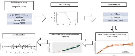
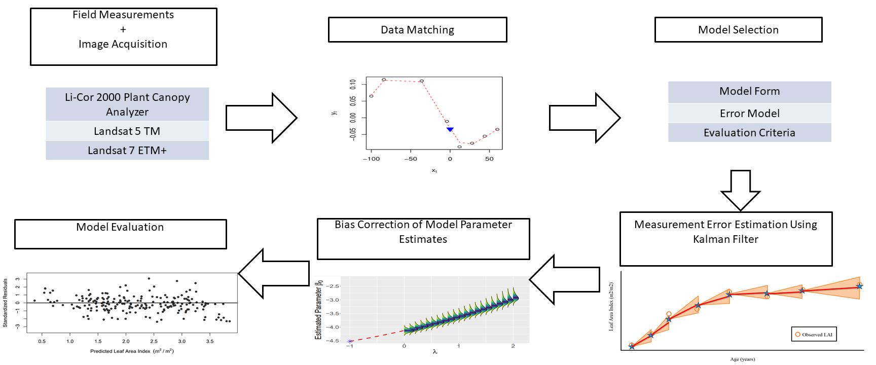
2. Materials and Methods
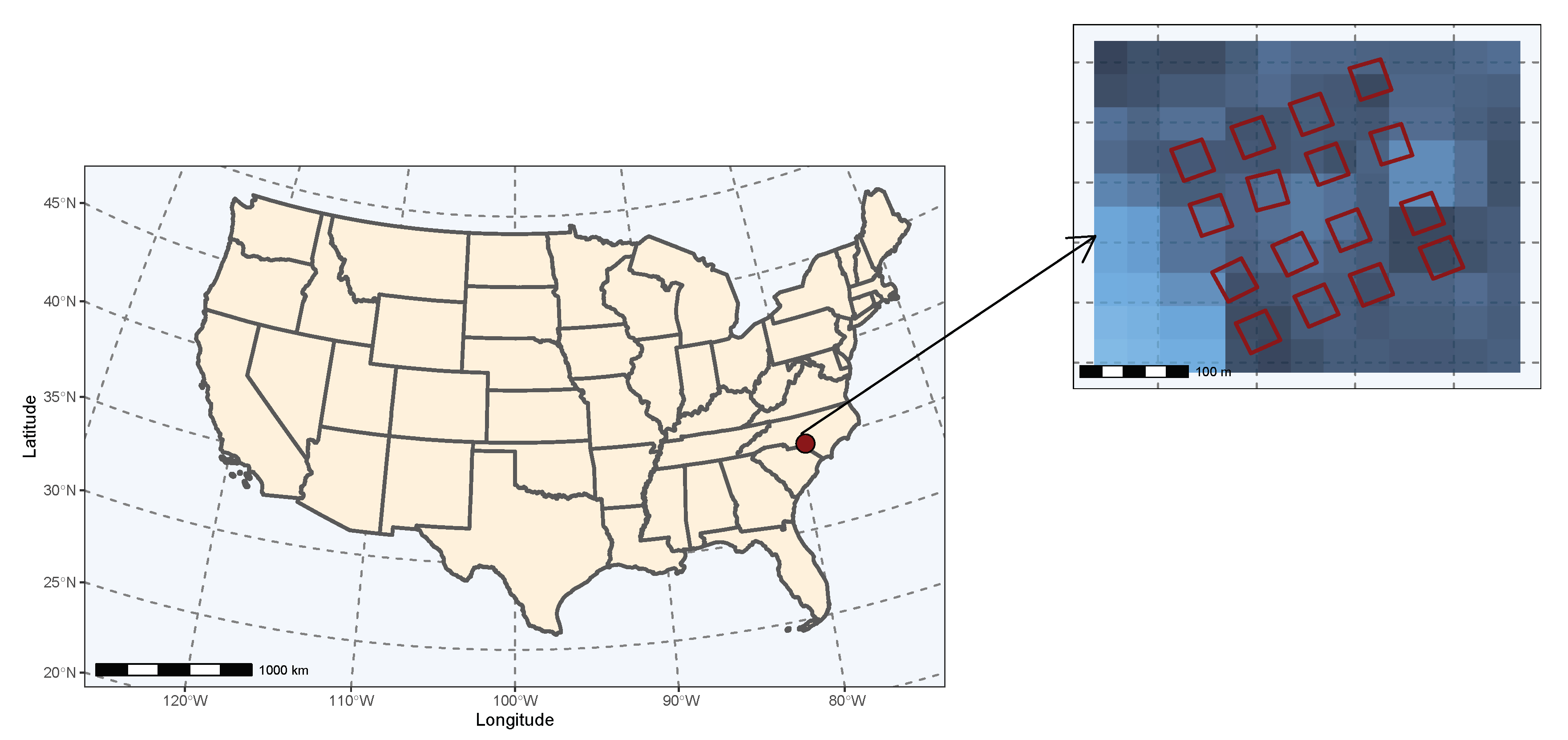
2.1. Study Site

For this study, we used leaf area index measurements taken at the Southeast Tree Research and Education Site (SETRES) study. The study was established in 1992 on a flat, excessively well drained loblolly pine plantation in Scotland County, North Carolina with an initial density of 1667 trees per hectare (2 m × 3 m spacing) (Figure 1). A total of sixteen 50 m × 50 m treatment plots were installed to cover four replications of a 2 × 2 factorial of irrigation and fertilization [19]. The study site’s 30-year annual precipitation average was 1210 mm and annual average temperature was 17 C [19]. Complete study site details are documented in Albaugh et al. [19]. Plot LAI measurements were made using a Li-Cor 2000 Plant Canopy Analyzer and were remeasured from March 1992 to September 2004 for a total of 1673 samples for all 16 study plots [19,51]. The individual plot LAI measurements were the average of twenty LAI measurements sampled along a transect within each plot. The complete LAI sampling protocol is documented in Albaugh et al. [19]. The age range covered by the in situ LAI measurements was between 7 and 20 years old. Stand level attributes throughout the time of this study are reported in Albaugh et al. [28].

2.2. Satellite Data

Landsat 5 Thematic Mapper (TM) and Landsat 7 Enhanced Thematic Mapper Plus (ETM+) imagery were selected for this study due to the temporal overlap between in situ measurements and image dates. Landsat Level-1 Tier 1 products were used to ensure the highest radiometric and geometric calibration across sensors for time-series analysis. The Landsat Level-1 Tier 1 products were atmospherically corrected to provide surface reflectance data, correcting for atmospheric distortions and allowing for the comparison with the in situ measurements [5]. U.S. Geological Survey (USGS) Landsat 5 and 7 Surface Reflectance Level 1 Tier 1 data were queried in the Google Earth Engine from 1 January 1991 to 31 December 2005 [52]. Nadir BRDF-adjusted reflectance values were calculated using the c-factor approach to provide temporal and geographic consistency across the thirteen years of observation [40]. Data were further filtered to remove cloud and shadow anomalies based on quality assurance bands and excessive haziness based on the atmospheric opacity band. Using individual polygons for the 16 study plots, the weighted average of the within plot pixel values was calculated and returned to account for the study plots covering multiple partial pixels. Above canopy satellite observations were paired to the in situ LAI estimates by matching observation dates. To account for the below canopy in situ LAI measurements that did not have matching satellite imagery sample dates, the four most previous and the four following satellite observations were subset and fitted with a thin plate spline. The thin plate spline was weighted by the associated standard deviation of the plot level reflectance summarization. The interpolated VI estimates and associated interpolation standard errors were extracted from the thin plate spline model for the in situ observation date. Using the interpolated and matched values, multiple vegetation indices were calculated using the individual band values for the polygons (Table 1) and fit to the paired in situ LAI estimate in a simple linear model form. The determination of the best performing VI to be used in the remainder of the methods occurred following the evaluation of all VIs in this step. VIs were evaluated on their correlation with LAI and the top performer is subsequently referred to as the “selected VI”.
Table 1. Vegetation indices evaluated in the analysis. Near-infrared (NIR), band 4 in Landsat 5 and 7 ETM+. Shortwave-infrared (SWIR), band 5 in Landsat 5 and 7 Enhanced Thematic Mapper + (ETM+). Shortwave-infrared 2 (SWIR2), band 7 in Landsat 5 and 7 ETM+.
Vegetation IndexEquationSource
Normalized Difference Vegetation Index (NDVI) NIR Red NIR + Red [34]
Simple Ratio (SR) NIR Red [35]
Simple Ratio 2 (SR2) SWIR NIR [53]
Enhanced Vegetation Index (EVI) 2.5 NIR Red NIR + 6 Red 7.5 Blue + 1 [54]
Soil Adjusted Vegetation Index (SAVI) 1.5 NIR Red NIR + Red + 0.5 [55]
Modified Soil Adjusted Vegetation Index (MSAVI) 2 NIR + 1 ( 2 NIR + 1 ) 2 8 ( NIR Red ) 2 [56]
Normalized Difference Moisture Index (NDMI) NIR SWIR NIR + SWIR [57]
Normalized Burn Index (NBI) NIR SWIR 2 NIR + SWIR 2 [58]
Chlorophyll Index Green (CIG) NIR Green 1 [59]
Modified Chlorophyll Absorption in Reflectance Index (MCARI) 1.2 ( 2.5 NIR Red 1.3 NIR Green ) [60]
Modified Chlorophyll Absorption in Reflectance Index 2 (MCARI2) 1.5 2.5 NIR Red 1.3 NIR Green ( 2 NIR + 1 ) 2 ( 6 NIR 5 Red 0.5 ) [60]
Pan Normalized Difference Vegetation Index (PanNDVI) NDVI ( Blue + Green + Red ) NDVI + ( Blue + Green + Red ) [61]
Green Ratio Vegetation Index (GR) NIR Green [62]

2.3. LAI Estimation Model

The model used the annual peak leaf area index (pLAI) values for each plot. The pLAI values, which typically occurred in August or September of any given year in the study, were identified and subset at the individual plot and year level to provide a series of pLAI values for each of the 16 plots, for a total of 208 pLAI observations. The pLAI data were randomly split into individual training (n = 156) and validation (n = 52) sets. Using the selected VI and observed pLAI, several linear, segmented, and nonlinear models were fit to the training data using the maximum likelihood framework (Table 2). Two segmented regression models were fit to the data set (Models 2 and 3, Table 3). The segmented models included a linear and nonlinear component, joined at a common point ( θ ) such that the line was continuous and smooth across the join point. To test the effect of silviculture on model performance, an indicator variable referred to as FERT, was included in several of the models to denote if the area under evaluation is under optimum nutrition management (1) or not (0) depending on the study treatment it is receiving. The variance structure was assumed to be non-constant for all but two models, Models 0 and 2 (Table 2). Model selection was based on information criterion (Akaike’s and Bayesian) and minimizing root mean square error (RMSE) ( 1 n ) i = 1 n ( y i x i ) 2 . During the model testing and diagnostics procedures, one pLAI observation was found to be highly influential and was removed from the training pLAI data set (n = 155).

2.4. Measurement Error Estimation

To estimate the amount of measurement error associated with the selected VI, the Kalman filter was used to step through the series of observations at each plot to determine the amount of error associated with the measurements and selected model. The Kalman filter, a recursive algorithm for data processing, provides mean and variance estimates of a known process under the influence of process and measurement errors through an iterative modeling process [63,64,65]. The selected VI values were fit to a three-parameter logistic equation (Equation (1)) to model the overall trend of the asymptotic VI development observed at the plot level from the multitemporal observations [65]:
V ( t ) = α 1 + e β t γ
where α is the asymptotic maximum value for VI, β is the location parameter for rate increase, γ is the shape parameter of the relation, t is time, and V is the VI. The Kalman filter utilized the algebraic differenced form of the equation (Equation (2)) to provide one step ahead estimates of VI for data with different starting points:
V ( t + i ) = V ( t ) 1 + e β ( t + i ) γ 1 + e β t γ
The generalized form of model was used to incorporate process error into the formula:
V ( t + i ) N V ( t ) 1 + e β t γ 1 + e β ( t + i ) γ , σ p r o c 2
Using the generalized formulation (Equation (3)), the VI for time n was projected using initial starting parameters, followed by an updated variance estimate. A new VI measurement was observed and input into the system. The observed measurement and projected estimate were assimilated, weighted by the inverse of their variances. The assimilated value was the new estimate of VI and the process was repeated by projecting it forward in time along with a variance update until the next VI observed measurement time. The recursive process was repeated until the system state was optimal given a set of constraints, which in this case minimized the negative log-likelihood. Output from the Kalman filter included updated estimates of the equation parameters in addition to estimates of the process and observation error.

2.5. Bias Correction
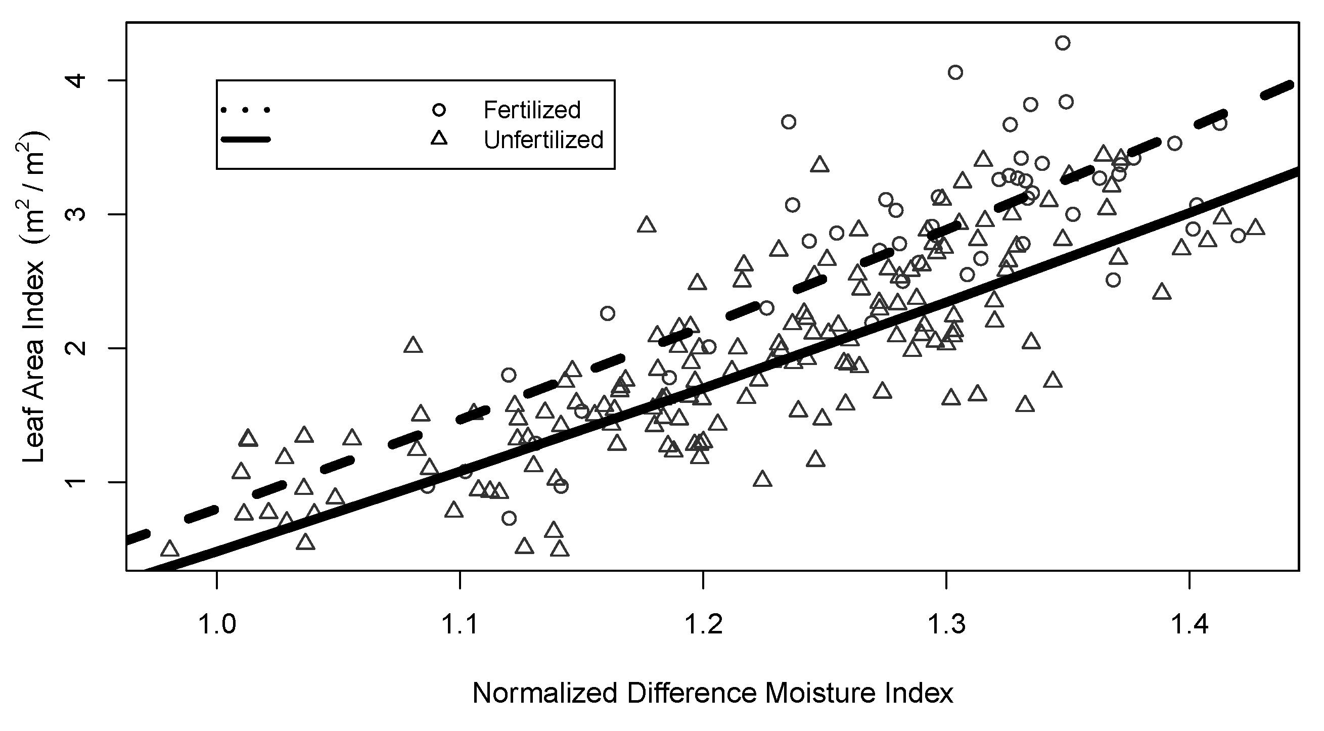
To correct for the effects of measurement error on the parameter estimates from VI observations, an error invariable approach was used to account for the fact that observations in the analysis come with errors. SIMEX was chosen as the methodology to solve this errors-in-variables issue due to its heuristic based approach for reducing biased parameters [66]. SIMEX permits flexibility in modeling because it does not require specifying an error structure model or a ranking of groups [48,66]. SIMEX, a simulation-based, error invariant method of manipulating the estimated model parameters to reduce the effects of measurement errors, can reduce bias in models with measurement error-prone variables [50,67,68]. The Kalman filter estimate of observation error associated with the selected VI time series for all 16 plots was used in conjunction with the interpolation errors in the SIMEX algorithm to correct for bias in the initial model parameters. SIMEX works with two main steps: a simulation step and an extrapolation step. Using the initial estimate of measurement variance and fitted parameters, SIMEX simulates increasing amounts of variance in the data and re-parameterizes the model. After several iterations of re-parameterizing the model with inflated variance, SIMEX extrapolates across the estimated (and biased) parameters to find the parameters with no variance [50,67]. To implement the SIMEX algorithm, the selected model and framework were refit with modified observations simulated to represent the inflated observation error estimate [69]. To create these modified observations, synthetic noise ( U ( λ l ) * ) was generated following U ( λ l ) * I I D N ( 0 , λ l σ 2 ) and was added to the observation [69]. The values for λ l ranged from 0 to 2 and were used to weight the amount of generated noise being added to the observation. A total of twenty steps between 0 and 2 were simulated 1000 times each for λ l . After simulating the observation error inflation, the refit coefficients were averaged for each λ l and plotted against the observation error values. A quadratic linear model was fit to correlate the new coefficient values to the λ l . The unbiased estimates were then extrapolated from the trend to the value of −1, as if the observations were measured completely without error.
To evaluate the robustness of the methodology and the predictive power of the model, the SIMEX parameter estimates were used to calculate mean square error (MSE) ( 1 n ) i = 1 n ( y i x i ) 2 on the training data set and mean square prediction error (MSPR) E i = 1 n g ( x i ) g ^ ( x i ) 2 on the validation data set. If MSE and MSPR comparisons are reasonable, the methodology is repeated with a combination of the two data sets.
To compare the proposed model to the current industry standard for LAI estimation from Landsat 5 TM/7 ETM+ imagery, the same procedures for handling in situ LAI measurements without exact satellite imagery matches were followed, Landsat 5 and 7 Top of Atmosphere (TOA) data were queried, matched, and interpolated to find corresponding SR values. Using the Flores et al. [11] model, LAI was estimated and compared to observed LAI.

3. Results

A total of 1673 measured observations were used to test the relationship between LAI and the individual vegetation indices. Of the 1673 observations, 1546 did not have exact date matches between in situ LAI measurements and satellite imagery (92%). The VI with the highest correlation with LAI was the normalized difference moisture index (NDMI), with a Pearson’s r value of 0.765, indicating a strong positive relationship, followed by simple ratio 2 (SR2), −0.756, and the simple ratio (SR), 0.735. When fitted to the 1673 observations, the relationship between NDMI and LAI had an adjusted R2 of 0.6172 (Figure 2). For this study, we shifted NDMI by one to be in the positive domain. September (n = 125) and August (n = 54) had the highest frequency of pLAI values (Figure 3).
Little improvement was observed in model performance as order increased and form changed as compared to the simple linear model until the treatment variable was included (Table 3). The model that best estimated pLAI based on lowest AIC, BIC, and RMSE using was Model 9 (Table 3). In addition to including NDMI, Model 9 included an indicator variable for FERT, referring to the optimum nutrition treatment that was applied to the fertilization and combination plots. With FERT in the model, a slight diverging relationship was observed in estimated LAI between the fertilized and unfertilized plots (Figure 4). The unfertilized plots maintained an overall linear relationship between the two variables, with lower expected LAI for a given NDMI as compared to the fertilized plots.
The addition of FERT into the model improved performance as seen by reductions in AIC and RMSE (Table 3). Using Model 6 as an example, the addition of FERT (Model 7) reduced RMSE by 0.0877 units of LAI, decreasing the AIC from 221.74 to 173.42. A further reduction in AIC and RMSE occurred from the change in how FERT was incorporated into the model (Table 3). Model 9 used a nonlinear function of the VI to model the effect of FERT rather than as a constant, reducing the overall RMSE to 0.3947 and AIC to 163.15 (Table 3).
Estimated observation error for the individual treatments were combined following additive error propagation protocol to a final estimate of 0.0019 units NDMI ( σ o b s 2 ). The SIMEX algorithm modified and unbiased the intercept and slope coefficient values to reduce the effects of measurement error in the NDMI estimation model, Model 9 (Table 3 (Figure 5)). The effects of increasing the amount of measurement error, or noise, on the individual parameters influenced how the parameters behaved, with well-defined trends in not only the mean value from the simulations, but also in the distribution of the parameter values in the simulations. For example, for β 0 , as λ increases from 0 to 2, the mean estimates for β 0 increase from approximately −4.12 to −2.91, while standard deviations increased from approximately 0.04 to 0.10 (Figure 5).
The calculated training dataset MSPR was 0.1431, and smaller than the calculated MSE on the training data set (0.1651), indicating that the model provided reasonable predictions. The combined model including the training and validation data (n = 207) provided the final model with unbiased parameters:
L A I = 4.520 + 4.930 NDMI + 0.271 NDMI 1.816 FERT 1 0.149 NDMI
With a model for the associated standard deviation (SD):
S D ( L A I ) = 0.156 NDMI 0.165
Residual analysis for the model showed no heteroskedasticity and no obvious bias comparing predicted and observed LAI across all observed levels of LAI (Figure 6 and Figure 7). The final MSE for the unbiased model was 0.1748 units of LAI (m2/m2) and RMSE was 0.4181 units of LAI (m2/m2).
Comparisons to the Flores et al. [11] model showed an overall underprediction of LAI as compared to the observed, with a calculated RMSE of 1.47 (Figure 7).

4. Discussion

NDMI was a better predictor of LAI in loblolly pine plantations in the southeastern United States when compared to more commonly used vegetation indices, such as NDVI and SR, supporting the findings in [70]. Whereas literature has supported the use of NDMI to predict vegetation density and canopy moisture, the authors of [71] hypothesized that the shortwave infrared band reflectance is more sensitive to shadows in the image, warranting further investigation of the various influences of canopy geometry on NDMI [57]. Other literature has supported the use of short wave infrared vegetation indices in retrieving canopy physiological properties, providing greater sensitivity to canopy moisture and vegetation anomalies, especially in drought prone areas [72,73,74]. NDMI, calculated by the difference ratio between near infrared (0.76–0.90 µm) and shortwave infrared (1.55–1.75 µm) bands, was a good predictor of live leaf biomass, total aboveground biomass, leaf moisture, and canopy moisture in other species [57,74,75,76]. Compared with the near-infrared band’s propensity to be reflected by the canopy, the shortwave infrared band wavelengths are absorbed by water, providing a measure of water (or moisture) content on the surface of interest [77,78]. The shortwave infrared band is sensitive to vegetation density in forests and to total biomass (brown and green), which is what plant canopy analyzers, such as the Li-Cor 2000, actually measure [71]. Optimum nutrition management influenced the behavior of the vegetation indices. Changes in the relationship between the VI and LAI when under optimum nutrition management may be a result of the increased photosynthetic capacity of the canopy, changes in leaf morphology, or allometric changes within stand [79,80,81]. Physical or physiological changes, such as transpiration, chlorophyll concentrations, foliar elemental concentrations, radiation use efficiency, or leaf size and orientation, may be the driving force behind the fertilization effect [39,80,82,83,84]. In other crops, a fertilization effect on plant spectral reflectance properties has been observed in the near-infrared and middle infrared wavelengths, with increases in reflectance for the middle infrared and decreases for the near-infrared when nitrogen fertilization had been applied [85,86,87]. Using the study level average reflectance for plots receiving (1) and not receiving (0) fertilization treatments, our study showed similar results, with decreased reflectance of the middle infrared band (Band 5 in Landsat 5 and 7), and increased reflectance in in the near infrared (Band 4) (Figure 8).
Using error invariable methods to correct for observations with error is a necessary step to provide unbiased estimators for modeling remotely sensed data. The SIMEX algorithm provided a flexible method for estimating the effects of increasing amounts of error on the individual parameters for the selected model, allowing for the extrapolation of the trend to find the value of the unbiased parameter. Including the estimated error for the interpolated values due to temporal misregistration and the overall process error represents two ways to account for the several sources of error that may affect remotely sensed data [49]. Overall, estimated errors from the Kalman filter and thin plate spline interpolations were relatively low, resulting in a slight change in model fit (Figure 9). Accounting for the errors in remotely sensed data provides the means to avoid violating the basic assumptions of linear modeling and reduces the influence of error prone variables.
While the data in this study come from a relatively small geographical area, the high temporal sampling provided a great number of LAI observations for the 16 plots. Note that the treatments applied in this study are not considered operational for loblolly pine plantations in the southeastern U.S. Consequently, our results may not well represent the relationship between remotely sensed VIs and observed LAI measurements in operational settings. However, the measured experimental data covers the range of LAI observed in operational plantations giving some confidence that these data would be useful to forest managers. The long timeline of this study may also introduce errors due to orbit drift in Landsat 5 for which we did not explicitly manage [88,89]. The study plots were relatively small compared to the pixel size used by Landsat imagery. The 50 m by 50 m measurement plot size did not allow for adequate sampling of the 30 m Landsat pixels to reduce spatial autocorrelation between pixels, for which a 3 by 3 pixel sampling area is recommended [49]. New sensors with higher resolution imagery will provide better sampling of the small study plots typically used for forestry research and should avoid this issue. While the weighted average of the pixels falling within the study plot were used to calculate the VIs, a further potential source of errors may come from interference in reflectance from areas surrounding the study plot under evaluation. Results from [90] corroborate the general underprediction of [11], thus the model presented in this research (Equation (4)) should provide an update to sites relying on legacy data from Landsat 5 TM and 7 ETM+. Further improvements in leaf area index predictions may be realized through the use of advanced machine learning techniques, but the ease of use was the driving force behind the development of the model proposed in this research. Furthermore, the framework for reducing the effects of observation errors provided in this research can be applied to new sensors, such as Landsat-8 and Sentinel-2, providing up to date imagery of current plantations.

5. Conclusions

This study used error-in-variable methods to reduce the effects of measurement errors in a leaf area index estimation model from Landsat 5 and 7 satellite imagery. A difference equation using shortwave infrared and near-infrared bands was the vegetation index with the highest correlation to in situ loblolly pine plantation leaf area index measurements (76.4%). A model form including an indicator variable for optimum nutrition management was the best framework for modeling the relationship between NDMI and LAI, achieving a RMSE of 0.4181 (m2/m2). The Kalman filter was used to quantify the amount of measurement error associated with the vegetation index, 0.0019 units NDMI. SIMEX provided a methodology to reduce the effects of vegetation index measurement error on the final model parameter estimates by establishing a relationship between increasing amounts of error and its subsequent effect on parameter behavior. The proposed model provides an improvement in loblolly pine plantation LAI estimation across the Landsat 5 TM and 7 ETM+ time frame in the southeastern United States. The improvement in spatial and temporal LAI retrieval increases the understanding of forest productivity by providing historical context to the development of loblolly pine plantations allowing for better management of forest resources.

Author Contributions

Conceptualization, C.R.M.; data curation: T.J.A.; methodology, C.R.M., D.R.M., and S.M.K.; formal analysis, S.M.K.; writing—original draft preparation, S.M.K.; writing—review and editing, S.M.K., C.R.M., T.J.A., and D.R.M.; funding acquisition, C.R.M. All authors have read and agreed to the published version of the manuscript.

Funding

This project was funded by the Plantation Management Research Cooperative and the McIntire-Stennis project GEOZ-0180-MS.

Acknowledgments

We gratefully acknowledge support provided by the Forest Productivity Cooperative and the Department of Forest Resources and Environmental Conservation at Virginia Polytechnic Institute and State University. Funding for this work was provided in part by the Virginia Agricultural Experiment Station and the McIntire-Stennis Program of the National Institute of Food and Agriculture, U.S. Department of Agriculture. This study was supported in part by resources and technical expertise from the Georgia Advanced Computing Resource Center, a partnership between the University of Georgia’s Office of the Vice President for Research and Office of the Vice President for Information Technology.

Conflicts of Interest

The authors declare no conflict of interest.

References

  1. Waring, R. Estimating Forest Growth and Efficiency in Relation to Canopy Leaf Area. In Advances in Ecological Research; MacFadyen, A., Ford, E., Eds.; Academic Press: Cambridge, MA, USA, 1983; Volume 13, pp. 327–354. [Google Scholar] [CrossRef]
  2. Shi, K.; Cao, Q.V. Predicted leaf area growth and foliage efficiency of loblolly pine plantations. For. Ecol. Manag. 1997, 95, 109–115. [Google Scholar] [CrossRef]
  3. Gower, S.T.; Kucharik, C.J.; Norman, J.M. Direct and indirect estimation of leaf area index, fAPAR, and net primary production of terrestrial ecosystems. Remote Sens. Environ. 1999, 70, 29–51. [Google Scholar] [CrossRef]
  4. Claverie, M.; Vermote, E.F.; Franch, B.; Masek, J.G. Evaluation of the Landsat-5 TM and Landsat-7 ETM+ surface reflectance products. Remote Sens. Environ. 2015, 169, 390–403. [Google Scholar] [CrossRef]
  5. Masek, J.G.; Vermote, E.F.; Saleous, N.E.; Wolfe, R.; Hall, F.G.; Huemmrich, K.F.; Gao, F.; Kutler, J.; Lim, T.K. A Landsat surface reflectance dataset for North America, 1990–2000. IEEE Geosci. Remote. Sens. Lett. 2006, 3, 68–72. [Google Scholar] [CrossRef]
  6. Flores, F.J. Using Remote Sensing Data To Estimate Leaf Area Index and Foliar Nitrogen of Loblolly Pine Plantations. Ph.D. Thesis, North Carolina State University, Raleigh, NC, USA, 2003. [Google Scholar]
  7. Fox, T.R.; Allen, H.L.; Albaugh, T.J.; Rubilar, R.; Carlson, C.A. Tree nutrition and forest fertilization of pine plantations in the southern United States. South. J. Appl. For. 2007, 31, 5–11. [Google Scholar] [CrossRef] [Green Version]
  8. Oswalt, S.N.; Smith, W.B.; Miles, P.D.; Pugh, S.A. Forest Resources of the United States, 2012: A Technical Document Supporting the Forest Service 2010 Update of the RPA Assessment; General Technical Report WO-91; US Department of Agriculture, Forest Service: Washington, DC, USA, 2014; 218p. [CrossRef]
  9. Parresol, B.R.; Scott, D.A.; Zarnoch, S.J.; Edwards, L.A.; Blake, J.I. Modeling forest site productivity using mapped geospatial attributes within a South Carolina Landscape, USA. For. Ecol. Manag. 2017, 406, 196–207. [Google Scholar] [CrossRef]
  10. Coleman, T.; Gudapati, L.; Derrington, J. Monitoring forest plantations using Landsat Thematic Mapper data. Remote Sens. Environ. 1990, 33, 211–221. [Google Scholar] [CrossRef]
  11. Flores, F.J.; Allen, H.L.; Cheshire, H.M.; Davis, J.M.; Fuentes, M.; Kelting, D. Using multispectral satellite imagery to estimate leaf area and response to silvicultural treatments in loblolly pine stands. Can. J. For. Res. 2006, 36, 1587–1596. [Google Scholar] [CrossRef] [Green Version]
  12. Iiames, J.S.; Congalton, R.G.; Pilant, A.N.; Lewis, T.E. Leaf area index (LAI) change detection analysis on loblolly pine (Pinus taeda) following complete understory removal. Photogramm. Eng. Remote Sens. 2008, 74, 1389–1400. [Google Scholar] [CrossRef] [Green Version]
  13. Iverson, L.R.; Graham, R.L.; Cook, E.A. Applications of satellite remote sensing to forested ecosystems. Landsc. Ecol. 1989, 3, 131–143. [Google Scholar] [CrossRef]
  14. Sivanpillai, R.; Smith, C.T.; Srinivasan, R.; Messina, M.G.; Wu, X.B. Estimation of managed loblolly pine stand age and density with Landsat ETM+ data. For. Ecol. Manag. 2006, 223, 247–254. [Google Scholar] [CrossRef]
  15. Stein, B.R.; Thomas, V.A.; Lorentz, L.J.; Strahm, B.D. Predicting macronutrient concentrations from loblolly pine leaf reflectance across local and regional scales. GISci. Remote Sens. 2014, 51, 269–287. [Google Scholar] [CrossRef] [Green Version]
  16. Yang, Y.; Anderson, M.C.; Gao, F.; Hain, C.R.; Semmens, K.A.; Kustas, W.P.; Noormets, A.; Wynne, R.H.; Thomas, V.A.; Sun, G. Daily Landsat-scale evapotranspiration estimation over a forested landscape in North Carolina, USA, using multi-satellite data fusion. Hydrol. Earth Syst. Sci. 2017, 21, 1017–1037. [Google Scholar] [CrossRef] [Green Version]
  17. Blinn, C.E.; Albaugh, T.J.; Fox, T.R.; Wynne, R.H.; Stape, J.L.; Rubilar, R.A.; Allen, H.L. A Method for Estimating Deciduous Competition in Pine Stands Using Landsat. South. J. Appl. For. 2012, 36, 71–78. [Google Scholar] [CrossRef]
  18. Vose, J.M.; Allen, H.L. Leaf area, stemwood growth, and nutrition relationships in loblolly pine. For. Sci. 1988, 34, 547–563. [Google Scholar] [CrossRef]
  19. Albaugh, T.J.; Allen, H.L.; Dougherty, P.M.; Kress, L.W.; King, J.S. Leaf area and above- and belowground growth responses of loblolly pine to nutrient and water additions. For. Sci. 1998, 44, 317–328. [Google Scholar] [CrossRef]
  20. Peduzzi, A.; Wynne, R.H.; Fox, T.R.; Nelson, R.F.; Thomas, V.A. Estimating leaf area index in intensively managed pine plantations using airborne laser scanner data. For. Ecol. Manag. 2012, 270, 54–65. [Google Scholar] [CrossRef] [Green Version]
  21. Monteith, J.L. Solar Radiation and Productivity in Tropical Ecosystems. J. Appl. Ecol. 1972, 9. [Google Scholar] [CrossRef] [Green Version]
  22. Vose, J.M.; Swank, W.T. A Conceptual Model of Forest Growth Emphasizing Stand Leaf Area. In Process Modeling of Forest Growth Responses to Environmental Stress; Dixon, R.K., Meldahl, R.S., Ruark, G.A., Warren, W.G., Eds.; Timber Press, Inc.: Portland, OR, USA, 1990; pp. 278–287. [Google Scholar]
  23. Mahowald, N.; Lo, F.; Zheng, Y.; Harrison, L.; Funk, C.; Lombardozzi, D.; Goodale, C. Projections of leaf area index in earth system models. Earth Syst. Dyn. 2016, 7, 211–229. [Google Scholar] [CrossRef] [Green Version]
  24. Teskey, R.O.; Bongarten, B.C.; Cregg, B.M.; Dougherty, P.M.; Hennessey, T.C. Physiology and genetics of tree growth response to moisture and temperature stress: An examination of the characteristics of loblolly pine (Pinus taeda L.). Tree Physiol. 1987, 3, 41–61. [Google Scholar] [CrossRef]
  25. Jokela, E.J.; Martin, T.A. Effects of ontogeny and soil nutrient supply on production, allocation, and leaf area efficiency in loblolly and slash pine stands. Can. J. For. Res. 2000, 30, 1511–1524. [Google Scholar] [CrossRef]
  26. Gonzalez-Benecke, C.A.; Jokela, E.J.; Martin, T.A. Modeling the effects of stand development, site quality, and silviculture on leaf area index, litterfall, and forest floor accumulations in loblolly and slash pine plantations. For. Sci. 2012, 58, 457–471. [Google Scholar] [CrossRef]
  27. Dalla-Tea, F.; Jokela, E. Needlefall, Canopy Light Interception, and Productivity of Young Intensively Managed Slash and Loblolly Pine. For. Sci. 1991, 37, 1298–1313. [Google Scholar] [CrossRef]
  28. Albaugh, T.J.; Lee Allen, H.; Dougherty, P.M.; Johnsen, K.H. Long term growth responses of loblolly pine to optimal nutrient and water resource availability. For. Ecol. Manag. 2004, 192, 3–19. [Google Scholar] [CrossRef]
  29. Jokela, E.J.; Dougherty, P.M.; Martin, T.A. Production dynamics of intensively managed loblolly pine stands in the southern United States: A synthesis of seven long-term experiments. For. Ecol. Manag. 2004, 192, 117–130. [Google Scholar] [CrossRef]
  30. Sampson, D.A.; Amatya, D.M.; Lawson, C.D.B.; Skaggs, R.W. Leaf Area Index (LAI) of Loblolly Pine and Emergent Vegetation Following a Harvest. Trans. ASABE 2011, 54, 2057–2066. [Google Scholar] [CrossRef]
  31. Yang, W.; Tan, B.; Huang, D.; Rautiainen, M.; Shabanov, N.V.; Wang, Y.; Privette, J.L.; Huemmrich, K.F.; Fensholt, R.; Sandholt, I.; et al. MODIS leaf area index products: From validation to algorithm improvement. IEEE Trans. Geosci. Remote Sens. 2006, 44, 1885–1898. [Google Scholar] [CrossRef]
  32. Qi, J.; Kerr, Y.; Moran, M.; Weltz, M.; Huete, A.; Sorooshian, S.; Bryant, R. Leaf Area Index Estimates Using Remotely Sensed Data and BRDF Models in a Semiarid Region. Remote Sens. Environ. 2000, 73, 18–30. [Google Scholar] [CrossRef] [Green Version]
  33. Shoemaker, D.A.; Cropper, W.P. Prediction of leaf Area Index for Southern Pine Plantations from Satellite Imagery Using Regression and Artificial Neural Networks. In Proceedings of the 6th Southern Forestry and Natural Resources GIS Conference, Orlando, FL, USA, 24–26 March 2008; pp. 139–160. [Google Scholar]
  34. Rouse, J.; Hass, R.; Deering, D.; Shell, J.; Harlan, J. Monitoring the Vernal Advancement and Retrogradation (Green Wave Effect) of Natural Vegetation; Report; NASA: Washington, DC, USA, 1974.
  35. Chen, J.M.; Cihlar, J. Retrieving leaf area index of boreal conifer forests using landsat TM images. Remote Sens. Environ. 1996, 55, 153–162. [Google Scholar] [CrossRef]
  36. Wang, Q.; Adiku, S.; Tenhunen, J.; Granier, A. On the relationship of NDVI with leaf area index in a deciduous forest site. Remote Sens. Environ. 2005, 94, 244–255. [Google Scholar] [CrossRef]
  37. Qu, Y.; Zhuang, Q. Modeling leaf area index in North America using a process-based terrestrial ecosystem model. Ecosphere 2018, 9. [Google Scholar] [CrossRef] [Green Version]
  38. Curran, P. Multispectral remote sensing of vegetation amount. Prog. Phys. Geogr. Earth Environ. 1980, 4, 315–341. [Google Scholar] [CrossRef]
  39. Knipling, E.B. Physical and physiological basis for the reflectance of visible and near-infrared radiation from vegetation. Remote Sens. Environ. 1970, 1, 155–159. [Google Scholar] [CrossRef]
  40. Roy, D.; Zhang, H.; Ju, J.; Gomez-Dans, J.; Lewis, P.; Schaaf, C.; Sun, Q.; Li, J.; Huang, H.; Kovalskyy, V. A general method to normalize Landsat reflectance data to nadir BRDF adjusted reflectance. Remote Sens. Environ. 2016, 176, 255–271. [Google Scholar] [CrossRef] [Green Version]
  41. Vermote, E.; Tanre, D.; Deuze, J.; Herman, M.; Morcette, J.J. Second Simulation of the Satellite Signal in the Solar Spectrum, 6S: An overview. IEEE Trans. Geosci. Remote. Sens. 1997, 35, 675–686. [Google Scholar] [CrossRef] [Green Version]
  42. Huete, A.R.; Liu, H.Q.; van Leeuwen, W.J.D. The use of vegetation indices in forested regions: Issues of linearity and saturation. In Proceedings of the IGARSS’97, 1997 IEEE International Geoscience and Remote Sensing Symposium Proceedings. Remote Sensing—A Scientific Vision for Sustainable Development, Singapore, 3–8 August 1997; Volume 4, pp. 1966–1968. [Google Scholar]
  43. Huete, A.; Justice, C.; van Leeuwen, W. MODIS Vegetation Index (MOD 13) Algorithm Theoretical Basis Document; Report; NASA Goddard Space Flight Center: Greenbelt, MD, USA, 1999.
  44. Mutanga, O.; Skidmore, A.K. Narrow band vegetation indices overcome the saturation problem in biomass estimation. Int. J. Remote Sens. 2004, 25, 3999–4014. [Google Scholar] [CrossRef]
  45. Gholz, H.L. Crown and Canopy Structure in Relation to Productivity. In Crown and Canopy Structure in Relation to Productivity; Fujimori, T., Whitehead, D., Eds.; Forestry Products Research Institute: Ibaraki, Japan, 1986; pp. 224–242. [Google Scholar]
  46. Gitelson, A.A.; Kaufman, Y.J.; Merzlyak, M.N. Use of a green channel in remote sensing of global vegetation from EOS-MODIS. Remote Sens. Environ. 1996, 58, 289–298. [Google Scholar] [CrossRef]
  47. Lunetta, R.S.; Congalton, R.G.; Fenstermaker, L.K.; Jensen, J.R.; McGwire, K.C.; Tinny, L.R. Remote sensing and geographic information system data integration: Error sources and research issues. Photogramm. Eng. Remote Sens. 1991, 57, 677–687. [Google Scholar]
  48. Fernandes, R.; Leblanc, S.G. Parametric (modified least squares) and non-parametric (Theil–Sen) linear regressions for predicting biophysical parameters in the presence of measurement errors. Remote Sens. Environ. 2005, 95, 303–316. [Google Scholar] [CrossRef]
  49. Curran, P.J.; Hay, A.M. The importance of measurement error for certain procedures in remote sensing at optical wavelengths. Photogramm. Eng. Remote Sens. 1986, 52, 229–241. [Google Scholar]
  50. Cook, J.R.; Stefanski, L.A. Simulation-Extrapolation Estimation in Parametric Measurement Error Models. J. Am. Stat. Assoc. 1994, 89. [Google Scholar] [CrossRef]
  51. Li-Cor. LAI-2000 Plant Canopy Analyzer Instruction Manual; LI-COR Biosciences: Lincoln, NE, USA, 1991. [Google Scholar]
  52. Gorelick, N.; Hancher, M.; Dixon, M.; Ilyushchenko, S.; Thau, D.; Moore, R. Google Earth Engine: Planetary-scale geospatial analysis for everyone. Remote Sens. Environ. 2017, 202, 18–27. [Google Scholar] [CrossRef]
  53. Shibayama, M.; Salli, A.; Häme, T.; Iso-Iivari, L.; Heino, S.; Alanen, M.; Morinaga, S.; Inoue, Y.; Akiyama, T. Detecting Phenophases of Subarctic Shrub Canopies by Using Automated Reflectance Measurements. Remote Sens. Environ. 1999, 67, 160–180. [Google Scholar] [CrossRef]
  54. Huete, A.; Didan, K.; Miura, T.; Rodriguez, E.; Gao, X.; Ferreira, L. Overview of the radiometric and biophysical performance of the MODIS vegetation indices. Remote Sens. Environ. 2002, 83, 195–213. [Google Scholar] [CrossRef]
  55. Huete, A.R. A soil-adjusted vegetation index (SAVI). Remote Sens. Environ. 1988, 25, 295–309. [Google Scholar] [CrossRef]
  56. Qi, J.; Chehbouni, A.; Huete, A.R.; Kerr, Y.H.; Sorooshian, S. A modified soil adjusted vegetation index. Remote Sens. Environ. 1994, 48, 119–126. [Google Scholar] [CrossRef]
  57. Hardisky, M.; Klemas, V.; Smart, R. The influence of soil salinity, growth form, and leaf moisture on the spectral radiance of Spartina. Photogramm. Eng. Remote Sens. 1983, 49, 77–83. [Google Scholar]
  58. Key, C.H.; Benson, N.C. Landscape assessment (LA). In FIREMON: Fire Effects Monitoring and Inventory System; General Technical Report, RMRS-GTR-164; Lutes, D.C., Keane, R.E., Caratti, J.F., Key, C.H., Benson, N.C., Sutherland, S., Gangi, L.J., Eds.; US Department of Agriculture, Forest Service, Rocky Mountain Research Station: Fort Collins, CO, USA, 2006; pp. 1–55. [Google Scholar]
  59. Gitelson, A.A.; Viña, A.; Arkebauer, T.J.; Rundquist, D.C.; Keydan, G.; Leavitt, B. Remote estimation of leaf area index and green leaf biomass in maize canopies. Geophys. Res. Lett. 2003, 30. [Google Scholar] [CrossRef] [Green Version]
  60. Haboudane, D. Hyperspectral vegetation indices and novel algorithms for predicting green LAI of crop canopies: Modeling and validation in the context of precision agriculture. Remote Sens. Environ. 2004, 90, 337–352. [Google Scholar] [CrossRef]
  61. Wang, F.M.; Huang, J.F.; Tang, Y.L.; Wang, X.Z. New Vegetation Index and Its Application in Estimating Leaf Area Index of Rice. Rice Sci. 2007, 14, 195–203. [Google Scholar] [CrossRef]
  62. Gitelson, A.A.; Kaufman, Y.J.; Stark, R.; Rundquist, D. Novel algorithms for remote estimation of vegetation fraction. Remote Sens. Environ. 2002, 80, 76–87. [Google Scholar] [CrossRef] [Green Version]
  63. Kalman, R.E. A new approach to linear filtering and prediction problems. J. Basic Eng. 1960, 82, 35–45. [Google Scholar] [CrossRef] [Green Version]
  64. Maybeck, P.S. Stochastic Models, Estimation and Control: Volume 1; Academic Press, Inc.: New York, NY, USA, 1979. [Google Scholar]
  65. Montes, C.R. A Resource Driven Growth and Yield Model for Loblolly Pine Plantations. Ph.D. Thesis, North Carolina State University, Raleigh, NC, USA, 2012. [Google Scholar]
  66. Ponzi, E.; Keller, L.F.; Muff, S.; Hansen, T. The simulation extrapolation technique meets ecology and evolution: A general and intuitive method to account for measurement error. Methods Ecol. Evol. 2019, 10, 1734–1748. [Google Scholar] [CrossRef]
  67. Misumi, M.; Furukawa, K.; Cologne, J.B.; Cullings, H.M. Simulation–extrapolation for bias correction with exposure uncertainty in radiation risk analysis utilizing grouped data. J. R. Stat. Soc. Ser. C 2017, 67, 275–289. [Google Scholar] [CrossRef]
  68. He, W.; Yi, G.Y.; Xiong, J. Accelerated failure time models with covariates subject to measurement error. Stat. Med. 2007, 26, 4817–4832. [Google Scholar] [CrossRef]
  69. Lederer, W.; Seibold, H. Simex: SIMEX- And MCSIMEX-Algorithm for Measurement Error Models, R package version 1.5; 2013. [Google Scholar]
  70. Blinn, C.; House, M.; Wynne, R.; Thomas, V.; Fox, T.; Sumnall, M. Landsat 8 Based Leaf Area Index Estimation in Loblolly Pine Plantations. Forests 2019, 10, 222. [Google Scholar] [CrossRef] [Green Version]
  71. Horler, D.N.H.; Ahern, F.J. Forestry information content of Thematic Mapper data. Int. J. Remote Sens. 1986, 7, 405–428. [Google Scholar] [CrossRef]
  72. Caccamo, G.; Chisholm, L.; Bradstock, R.; Puotinen, M. Assessing the sensitivity of MODIS to monitor drought in high biomass ecosystems. Remote Sens. Environ. 2011, 115, 2626–2639. [Google Scholar] [CrossRef]
  73. Gu, Y.; Brown, J.F.; Verdin, J.P.; Wardlow, B. A five-year analysis of MODIS NDVI and NDWI for grassland drought assessment over the central Great Plains of the United States. Geophys. Res. Lett. 2007, 34. [Google Scholar] [CrossRef] [Green Version]
  74. Gao, B.C. NDWI—A normalized difference water index for remote sensing of vegetation liquid water from space. Remote Sens. Environ. 1996, 58, 257–266. [Google Scholar] [CrossRef]
  75. Tucker, C.J. Remote sensing of leaf water content in the near infrared. Remote Sens. Environ. 1980, 10, 23–32. [Google Scholar] [CrossRef]
  76. Ahamed, T.; Tian, L.; Zhang, Y.; Ting, K.C. A review of remote sensing methods for biomass feedstock production. Biomass Bioenergy 2011, 35, 2455–2469. [Google Scholar] [CrossRef]
  77. Wilson, E.H.; Sader, S.A. Detection of forest harvest type using multiple dates of Landsat TM imagery. Remote Sens. Environ. 2002, 80, 385–396. [Google Scholar] [CrossRef]
  78. Cibula, W.G.; Zetka, E.F.; Rickman, D.L. Response of thematic mapper bands to plant water stress. Int. J. Remote Sens. 1992, 13, 1869–1880. [Google Scholar] [CrossRef]
  79. Maier, C.A.; Palmroth, S.; Ward, E. Short-term effects of fertilization on photosynthesis and leaf morphology of field-grown loblolly pine following long-term exposure to elevated CO(2) concentration. Tree Physiol. 2008, 28, 597–606. [Google Scholar] [CrossRef]
  80. Gough, C.M.; Seiler, J.R.; Maier, C.A. Short-term effects of fertilization on loblolly pine (Pinus taeda L.) physloiogy. Plant Cell Environ. 2004, 27, 876–886. [Google Scholar] [CrossRef]
  81. King, J.S.; Albaugh, T.J.; Allen, H.L.; Kress, L.W. Stand-level allometry in Pinus taeda as affected by irrigation and fertilization. Tree Physiol. 1999, 19, 769–778. [Google Scholar] [CrossRef] [Green Version]
  82. Al-Abbas, A.H.; Barr, R.; Hall, J.D.; Crane, F.L.; Baumgardner, M.F. Spectra of Normal and Nutrient-Deficient Maize Leaves. Agron. J. 1974, 66, 16–20. [Google Scholar] [CrossRef] [Green Version]
  83. Martin, T.A.; Jokela, E.J. Developmental patterns and nutrition impact radiation use efficiency components in southern pine stands. Ecol. Appl. 2004, 14, 1839–1854. [Google Scholar] [CrossRef]
  84. Wightman, M.; Martin, T.; Gonzalez-Benecke, C.; Jokela, E.; Cropper, W.; Ward, E. Loblolly Pine Productivity and Water Relations in Response to Throughfall Reduction and Fertilizer Application on a Poorly Drained Site in Northern Florida. Forests 2016, 7, 214. [Google Scholar] [CrossRef] [Green Version]
  85. Walburg, G.; Bauer, M.E.; Daughtry, C.S.T.; Housley, T.L. Effects of Nitrogen Nutrition on the Growth, Yield, and Reflectance Characteristics of Corn Canopies1. Agron. J. 1982, 74, 677–683. [Google Scholar] [CrossRef] [Green Version]
  86. Ahlrichs, J.S.; Bauer, M.E. Relation of Agronomic and Multispectral Reflectance Characteristics of Spring Wheat Canopies1. Agron. J. 1983, 75, 987–993. [Google Scholar] [CrossRef] [Green Version]
  87. Hinzman, L.; Bauer, M.; Daughtry, C. Effects of nitrogen fertilization on growth and reflectance characteristics of winter wheat. Remote Sens. Environ. 1986, 19, 47–61. [Google Scholar] [CrossRef]
  88. Zhang, H.K.; Roy, D.P. Landsat 5 Thematic Mapper reflectance and NDVI 27-year time series inconsistencies due to satellite orbit change. Remote Sens. Environ. 2016, 186, 217–233. [Google Scholar] [CrossRef] [Green Version]
  89. Roy, D.P.; Li, Z.; Zhang, H.K.; Huang, H. A conterminous United States analysis of the impact of Landsat 5 orbit drift on the temporal consistency of Landsat 5 Thematic Mapper data. Remote Sens. Environ. 2020, 240, 111701. [Google Scholar] [CrossRef]
  90. Cohrs, C.W.; Cook, R.L.; Gray, J.M.; Albaugh, T.J. Sentinel-2 Leaf Area Index Estimation for Pine Plantations in the Southeastern United States. Remote Sens. 2020, 12, 1406. [Google Scholar] [CrossRef]
Figure 1. Location and study plot layout of the Southeast Tree Research and Education Site (SETRES) in Scotland County, North Carolina. The inset map shows the Landsat 5 Thematic Mapper pixel size and location in relation to the SETRES study layout.
Remotesensing 13 01140 g001
Figure 2. Relationship between the normalized difference moisture index (shifted by one to be in the positive domain) and leaf area index data fit to a simple linear model for all observed measurement points (n = 1673). Adjusted R2 for this relationship was 0.5837 and root mean square error was 0.5049.
Remotesensing 13 01140 g002
Figure 3. Peak leaf area index measurements for the sixteen Southeast Tree Research and Education Site (SETRES) plots in Scotland County, North Carolina over the study period (1992–2004). Peak leaf area index typically occurred in August or September of any given year.
Remotesensing 13 01140 g003
Figure 4. Equation (4) fit using the unbiased parameters estimated using the simulation-extrapolation (SIMEX) methodology. Sites under the optimum nutrition silviculture regime are designated as “Fertilized”.
Remotesensing 13 01140 g004
Figure 5. Results from the simulation-extrapolation (SIMEX) method for reducing the effects of measurement error on the parameter value for Model 9 to estimate normalized difference moisture index (NDMI). As error was increased from 0 to 2 ( λ ), 1000 simulations were conducted and the new parameters were recorded. A quadratic linear model was used to fit the simulations and extrapolate to a λ level of −1, as if there was no measurement error.
Remotesensing 13 01140 g005
Figure 6. Standardized residuals for predictions using Equation (4). Results show little evidence of heteroscedasticity, indicating good model performance.
Remotesensing 13 01140 g006
Figure 7. Predicted vs. measured leaf area index from the SIMEX bias-corrected model (Equation (4)) and a comparison to the Flores et al. top of atmosphere model predictions [11].
Remotesensing 13 01140 g007
Figure 8. Changes in average Landsat 5 TM and 7 ETM+ Band 4 (NIR) and Band 5 (SWIR) reflectance values by fertilization status across the 16 study plots at the Southeast Tree Research and Education Site (SETRES) in Scotland County, North Carolina. Points show the Landsat 5 TM and 7 ETM+ observations used in the study.
Remotesensing 13 01140 g008
Figure 9. Comparison of the unbiased (Equation (4)) and biased model parameter fits for the unfertilized (FERT = 0) segment of model 9.
Remotesensing 13 01140 g009
Table 2. Model forms and error structure evaluated using the normalized difference moisture index (NDMI) to predicted leaf area index (LAI). An indicator variable, FERT, is used to denote if the area under evaluation is under optimum nutrition management (1) or not (0).
Model NumberModel FormError Model
0 y i = β 0 + β 1 NDMI ρ
1 y i = β 0 + β 1 NDMI ρ 1 NDMI ρ 2
2 y i = β 0 + β 1 X i if X i θ γ 0 X i γ 1 if X i > θ ρ
3 y i = β 0 + β 1 X i if X i θ γ 0 X i γ 1 if X i > θ ρ 1 NDMI ρ 2
4 y i = β 0 + β 1 NDMI β 2 ρ 1 NDMI ρ 2
5 y i = β 0 + β 1 NDMI + β 2 NDMI 2 ρ 1 NDMI ρ 2
6 y i = β 0 + β 1 NDMI 1 + β 2 NDMI ρ 1 NDMI ρ 2
7 y i = β 0 + β 1 NDMI + β 2 FERT 1 + β 3 NDMI ρ 1 NDMI ρ 2
8 y i = β 0 + β 1 NDMI + β 2 NDMI 2 + β 3 FERT ρ 1 NDMI ρ 2
9 y i = β 0 + β 1 NDMI + ( α 1 NDMI α 2 ) FERT 1 + β 2 NDMI ρ 1 NDMI ρ 2
Table 3. Associated fit statistics and evaluation criteria for the models evaluated using the training data (n = 155).
Model NumberAICBICRMSEBias-LogLikNumber of Parameters
0227.74236.870.49482.05E-07110.873
1225.13237.300.4954−0.00117108.574
2233.94249.160.4983−0.00421111.975
3227.14245.400.4993−6.99E-05107.576
4223.92239.140.49472.15E-05106.965
5223.60238.810.4948−1.74E-05106.805
6224.46239.680.4950−4.29E-05107.235
7176.74195.000.4118−0.000482.376
8175.83194.090.41367.34E-0381.916
9167.82189.120.39888.28E-0476.917
Publisher’s Note: MDPI stays neutral with regard to jurisdictional claims in published maps and institutional affiliations.

