Sea Ice Concentration and Sea Ice Extent Mapping with L-Band Microwave Radiometry and GNSS-R Data from the FFSCat Mission Using Neural Networks

Abstract

CubeSat-based Earth Observation missions have emerged in recent times, achieving scientifically valuable data at a moderate cost. FSSCat is a two 6U CubeSats mission, winner of the ESA S³ challenge and overall winner of the 2017 Copernicus Masters Competition, that was launched in September 2020. The first satellite, ³Cat-5/A, carries the FMPL-2 instrument, an L-band microwave radiometer and a GNSS-Reflectometer. This work presents a neural network approach for retrieving sea ice concentration and sea ice extent maps on the Arctic and the Antarctic oceans using FMPL-2 data. The results from the first months of operations are presented and analyzed, and the quality of the retrieved maps is assessed by comparing them with other existing sea ice concentration maps. As compared to OSI SAF products, the overall accuracy for the sea ice extent maps is greater than 97% using MWR data, and up to 99% when using combined GNSS-R and MWR data. In the case of Sea ice concentration, the absolute errors are lower than 5%, with MWR and lower than 3% combining it with the GNSS-R. The total extent area computed using this methodology is close, with 2.5% difference, to those computed by other well consolidated algorithms, such as OSI SAF or NSIDC. The approach presented for estimating sea ice extent and concentration maps is a cost-effective alternative, and using a constellation of CubeSats, it can be further improved.

1. Introduction

Global warming is having a big impact on polar sea ice, notably in the Arctic ocean. Satellite observations make it possible to monitor the sea area covered by ice, i.e., Sea Ice Extent (SIE), which has been decreasing in recent years at a rate of 13.1% per decade [1]. While this has ecological implications, it also opens new commercial opportunities, such as the opening of the North route joining Asia, Europe and North America in a faster way. SIE algorithms are based on microwave radiometry observations at ~19 and 37 GHz frequencies [2]. These frequencies can discriminate between sea water and sea ice, which makes it possible to define the sea ice margin and the associated sea ice extent. SIE monitoring at Arctic scale has been possible since 1978 using large satellites embarking Microwave Radiometers (MWR).

Several approaches exist for retrieving Sea Ice Concentration (SIC), i.e., the percentage of ice present in a given point of the sea, or SIE maps. Process-based algorithms, i.e., building a physical model, for SIC usually use a multi-frequency tie-point approach [3], or matched filtering of the Delay Doppler Maps (DDM) generated from GNSS-R data has been used for SIE [4]. More recently, Neural Networks (NN)-based algorithms have also been used with results close to the traditional methods [5], and even SMOS L-band data has been used to determine Sea Ice Thickness (SIT) [6].

CubeSats have been proven to be a cost-effective alternative for technology demonstrators and scientific missions. Multi-platform missions [7], such as Planet [8] or Spire [9], are becoming a reality thanks to reduced CubeSats costs, improving notably the revisit time. FSSCat mission was launched on the 3 September 2020 [10,11]. The mission consists of two 6U Earth Observation CubeSats. The first one, ³Cat-5/A carries onboard the Flexible Microwave Payload-2 (FMPL-2) payload [12,13]. FMPL-2 is a dual L-band MWR and a Global Navigation Satellite System-Reflectometer (GNSS-R) implemented using a Software-Defined Radio. Its main objective is to monitor the sea ice over the poles. The second one, ³Cat-5/B, carries on board Cosine’s Hyperscout-2 visible and near-infrared (VNIR) and Thermal Infrared (TIR) hyperspectral imager [14].

The objective of this study is to develop a methodology for generating SIC and SIE maps of the Arctic and the Antarctic oceans using the FMPL-2 MWR and the GNSS-R data for latitudes above 60° North and South. NN-based algorithms are relatively easy to implement, can find non-linear dependencies among data, and can handle large datasets efficiently. Therefore, this methodology designs two different NNs to retrieve the SIC, and SIE map: a regression fit NN to estimate SIC maps and a classification NN for the SIE ones. The first NN takes MWR data to generate coarse-resolution (12.5 km) SIC and SIE maps, and then a second NN is proposed to combine GNSS-R and MWR data to provide a higher resolution (~250 m) map over the tracks of the GNSS-R specular reflection points. The maps presented cover all the retrieved data from FSSCat during the months of October and November 2020 after the commissioning phase. To assess the quality of the produced maps, the data is compared to Ocean and Sea Ice Satellite Application Facility (OSI SAF) SIC and SIE maps [15]. Furthermore, the total SIE area is computed to have an overall view of the magnitude of the differences.

After this introduction, this work is organized as follows. Section 2 describes the FFSCat data used to generate the SIC and SIE maps, along with the auxiliary data used to train the networks, i.e., the land cover fraction, and the land and sea surface temperatures, also known as skin temperature. Land cover is adopted from the Moderate-Resolution Imaging Spectroradiometer (MODIS) [16], and the daily skin temperature is extracted from the European Centre for Medium-Range Weather Forecasts (ECMWF) [17]. Section 2 also describes the proposed methodology. Section 3 presents and comments the results obtained with the presented algorithm and compares them with the products from other missions. Finally, in Section 4, the main conclusions are summarized.

2. Materials and Methods

This section describes the data used as inputs. First, the FSSCat data, the brightness temperature from MWR and the GNSS-R reflected data points. Second, two auxiliary data sets used to complement the inputs for SIC and SIE estimation.

2.1. FSSCat Data

The presented methodology uses the data coming from both sensors of the FMPL-2 payload. On the one hand, it uses the L-band brightness temperature collected by the MWR to generate full SIC and SIE maps of both poles, and on the other hand, the data points collected by GNSS-R are used to improve the resolution of the previously generated MWR maps over the specular reflection tracks.

2.1.1. Microwave Radiometer Data

As mentioned in Section 1, MWR data at K_u and K_a-bands are routinely used to determine SIC. In this work, FFSCat L-band MWR is the main input used, which has a sensitivity better than 1 K [12]. The data is pre-processed to deliver daily brightness temperature maps at polar scales considering the northern hemisphere and three-day maps for the southern hemisphere, due to a different acquisition strategy followed in each pole by ³Cat-5/A. As the radiometer tracks partially overlap in the cross-track dimension, wherever there is overlap, values are generated by averaging multiple 1D tracks [13] (p. 10,11). MWR data resolution is resampled from the original spatial resolution determined by the antenna footprint (350 × 500 km²) to an Equal-Area Scalable Earth (EASE) [18] grid of 12.5 km and then a seven-day moving average window is applied across the temporal dimension to get the full coverage. An example data product from FSSCat MWR used as an input by the algorithm presented in this work is illustrated in Figure 1.

2.1.2. GNSS-R Data

The shape of the Delay Doppler Maps (DDM) can be used to detect whether a pixel is ice or open water [4]. TDS-1 and CYGNSS GNSS-R receivers use a coherent integration time of 1 ms, and an incoherent integration time of 1 s, providing an along-track blurring of approximately ~6.5 km. More recently CYGNSS GNSS-R receivers have decreased the integration time to 0.5 s. FSSCat was designed with an incoherent integration time of only 40 ms, which provides a blurring of less than 260 m, about the size of the first Fresnel zone [11]. However, the shorter the integration time, the greater the noise level, which makes the difference of the DDM’s shape between open water and sea ice less evident, as most of the tails are buried in the noise level as illustrated in Figure 2a. Nonetheless, the wider DDM over water than over ice and the calibrated reflectivity (i.e., ratio between reflected and direct signal as defined in [19]) of the reflected GNSS-R signal are large enough to detect the transitions between sea and ice as show in Figure 14 of [13]. This effect can also be seen in Figure 2b, where the reflectivity of the signal increases when the track changes between the sea open water area to the thin and thick ice, defined for SIC larger than 30% and 70%, respectively, in the OSI SAF maps.

The elevation angle during the acquisition has an important impact on the received SNR of the reflection, as well, as shown in [20,21]. Therefore, in addition to the DDM and the SNR, these additional data are added to the algorithm. Moreover, the classification accuracy improves for large SNR. Therefore, the GNSS-R tracks were pre-processed to filter out reflections with poor SNR, or with inconsistent absolute Doppler frequencies, as shown in [12] and explained in [13].

2.2. Auxiliary Data

The FMPL-2 antenna footprint is ~350 × 500 km²; therefore, when the satellite crosses the coastline, the antenna temperature contains information from both land and sea. Land brightness temperature is higher than that over sea. Therefore, in coastal areas, the brightness temperature over the sea is contaminated by that of the land. This is partially corrected by using two auxiliary data sets: the land cover fraction and the Skin surface Temperature (ST). The Land Cover Fraction (LCF) represents the fraction of land present on the area surrounding a given pixel. The Land Cover (LC) maps are retrieved from MODIS data, and a mask is computed for water bodies: 1 if the pixel is land, 0 if the pixel is water. Therefore, the number of pixels (N_i) of the land cover maps that are inside the computed area, centered on a given point (i) of MWR data, are used to compute the land cover fraction maps as

$${\mathrm{LCF}}_{\mathrm{i}}={\displaystyle \sum }_{\mathrm{j}=1}^{\mathrm{N}}\frac{{\mathrm{LC}}_{\mathrm{j}}}{{\mathrm{N}}_{\mathrm{i}}}$$

(1)

for every pixel of the 12.5 km EASE grid used for the MWR data. As will be discussed in Section 3.1, the fraction area is not only computed for the antenna footprint, but also for a larger square box of 201 by 201 pixels. The resulting LCF maps can be seen in Figure 3.

The ST is the surface temperature in each pixel of the map. It is composed of the land surface temperature maps and the sea surface temperatures retrieved from the ECMWF database, and resampled into the same 12.5 km EASE grid. Figure 4 shows two examples of the ST maps used.

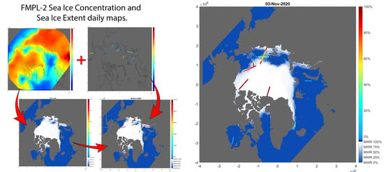
2.3. Sea Ice Concentration and Sea Ice Extent Retrieval Using Neural Networks

As mentioned in the previous sections, the main purpose of this work is to combine GNSS-R and MWR data from FSSCat by implementing and optimizing NNs to yield accurate maps of SIC and the associated with SIE at the polar scale. For both maps, the data from both sensors is combined in a two-step procedure. The first step uses the MWR and the auxiliary data as inputs of a NN to compute whether a pixel is ice or water. For the second step, the GNSS-R data analyzed with the NN supports the MWR data to conditionally enhance resolution whenever data at specular points is available. The maps generated in the first step have a spatial resolution of 12.5 km, and over them, the output points of the second step are placed in a non-gridded format in order to improve the resolution of the GNSS-R data (~250 m). SIC maps are generated following the same two steps of the SIE procedure but using a different NN.

2.3.1. Sea Ice Concentration and Extent Maps Based on MWR Data

To process the FMPL-2 MWR data, two NNs have been designed, in order to generate both SIC and SIE maps. For SIC maps, as SIC is a continuous variable from 0 to 100, an NN with continuous output is used to perform a regression fit of the input data [22]. The NN is designed as a fully connected Multilayer Perceptron network (MLP), where all the neurons for one layer are connected to the next one. Different networks with different number of hidden layers have been tested. Increasing the number of hidden layers increases the required training time, but it also improves the accuracy of the trained networks by ~1%, and it is affordable for actual computers. However, more than three hidden layers does not improve the results. After seeing the results, the chosen network was composed as follows:

• Input layer: 5 neurons;
• 3 hidden layers: consisting of 5, 10 and 5 neurons, respectively, using the sigmoid activation function;
• Output layer: a single neuron with a continuous linear output function;
• Each of the input neurons corresponds to one variable of the same point of the EASE grid. After a selection procedure described in Section 3, the 6 input variables are:
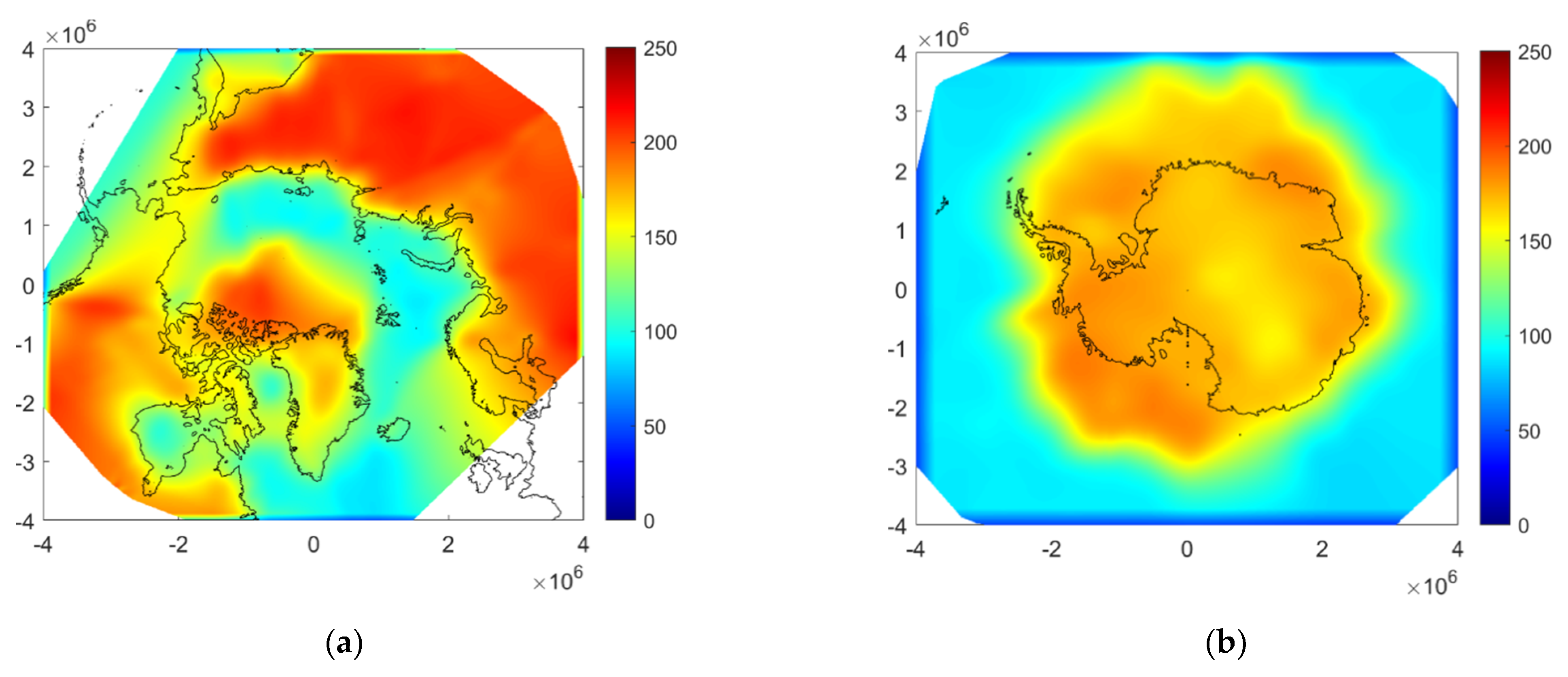
• Brightness temperature;
• Temporal standard deviation of the brightness temperature: Computed using 10 radiometry samples (5 s window);
• Gradient of the brightness temperature: Two inputs $\left(\nabla x, \nabla y\right)$, one for each axis;
• Land cover fraction; and
• Skin surface temperature.

In the case of the SIE maps, the NN architecture is different. It is an MLP network with the same number of inputs, and the same hidden layers as the SIC network, but the output layer consists of a single output with a binary classification output function. In both cases, a different NN is trained for each pole.

More than 5 million points of FMPL-2 MWR data for the Arctic, and more than 800 thousand for the Antarctic, are available to train the networks; therefore, to avoid overfitting [23], only a small fraction of these data, ~20,000 random samples for each pole, is used to train and validate the networks. The training methodology used in this work is the Levenberg-Marquardt method [24]. OSI SAF SIC products [15] are used as the ground truth to train the networks, resampled at the same 12.5 km EASE grid. Once the networks have been trained, all the data available is processed through them, and multiple maps from different time periods of both poles are generated with the same EASE grid used for the inputs.

2.3.2. Resolution Improvement Using GNSS-R

As mentioned in the previous sections, the algorithm uses the GNSS-R data as well to improve the resolution of the maps generated using the MWR data. A similar approach as the MWR is followed. A MLP classification NN for SIE and a continuous output NN for SIC, with three same hidden layers than the MWR case. However, the number of inputs is larger: for the GNSS-R data, 12 input neurons are used:

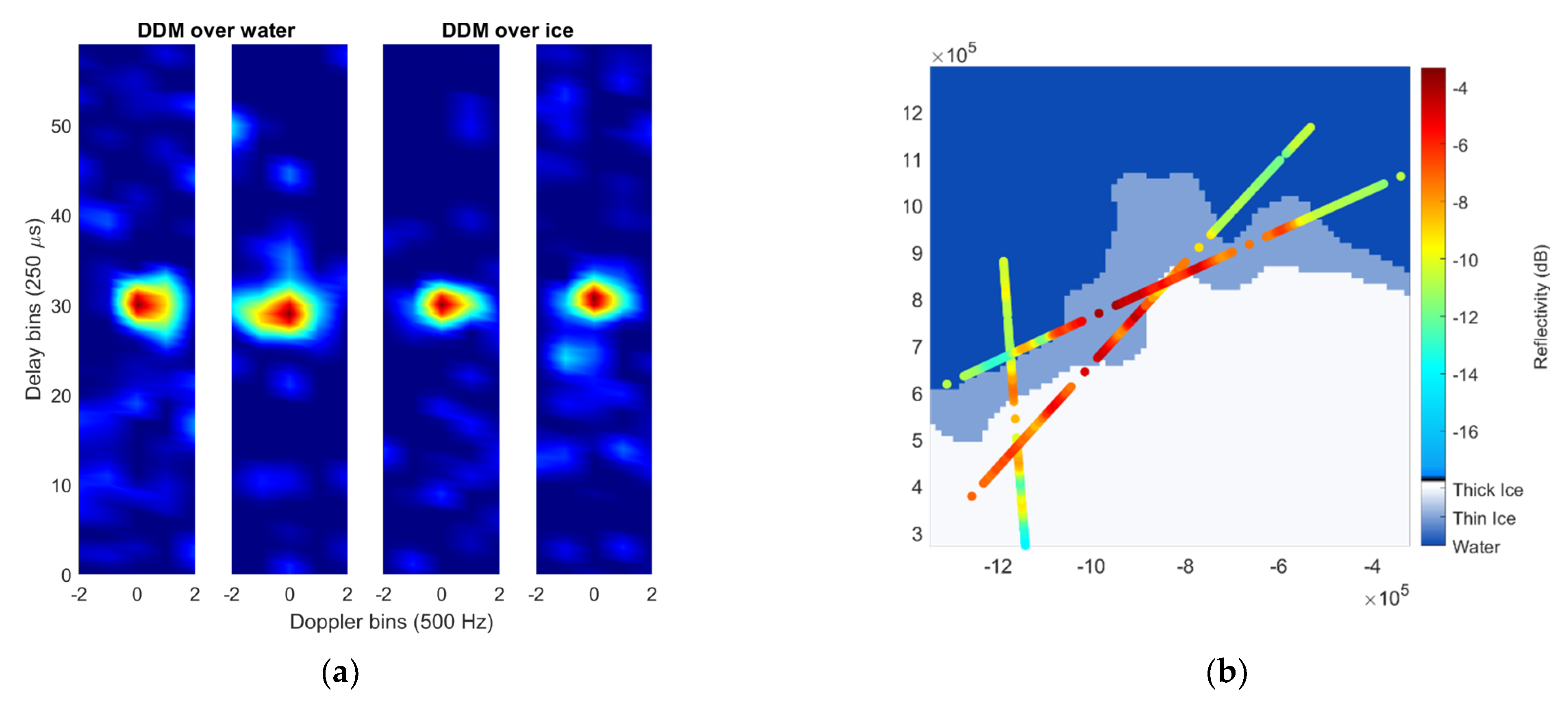
• Averaged Delay Doppler Map (ADDM): All the delay bins ($\mathrm{j}$) of the DDM are averaged and normalized, dividing by the peak averaged value:

  $${\langle \mathrm{DDM}\rangle }_{\mathrm{i}}=\frac{{{\displaystyle \sum }}_{\mathrm{j}=1}^{\mathrm{N}}\frac{{\mathrm{DDM}}_{\mathrm{i},\mathrm{j}}}{{\mathrm{N}}_{\mathrm{i}}}}{\max \left({{\displaystyle \sum }}_{\mathrm{j}=1}^{\mathrm{N}}\frac{{\mathrm{DDM}}_{\mathrm{i},\mathrm{j}}}{{\mathrm{N}}_{\mathrm{i}}}\right)}.$$

  (2)

Five input neurons are required to read this parameter, one for each Doppler bin ($\mathrm{i}$).

• Elevation angle of the reflected signal;
• Reflectivity;
• Standard deviation of the reflectivity;
• SNR;
• Brightness temperature: The FMPL-2 MWR brightness temperature for each point of the GNSS-R data is bilinearly interpolated into the specular reflection points;
• Land cover fraction: The LCF for each point is bilinearly interpolated into the specular reflection points; and
• Skin surface temperature: The ST for each point is bilinearly interpolated into the specular reflection points.

The same training methodology as in the MWR case is followed. Regarding the number of samples used to train and validate the network, in the GNSS-R case, fewer samples are available than for the MWR case; therefore, ~20,000 samples are used for the Arctic and ~5500 for the Antarctic. The ground truth is the same as before; however, as the brightness temperature, the OSI SAF data is scattered over the specular point using the same interpolation. Finally, the classified points are scattered over the generated maps using the MWR data to preserve the high resolution of the GNSS-R.

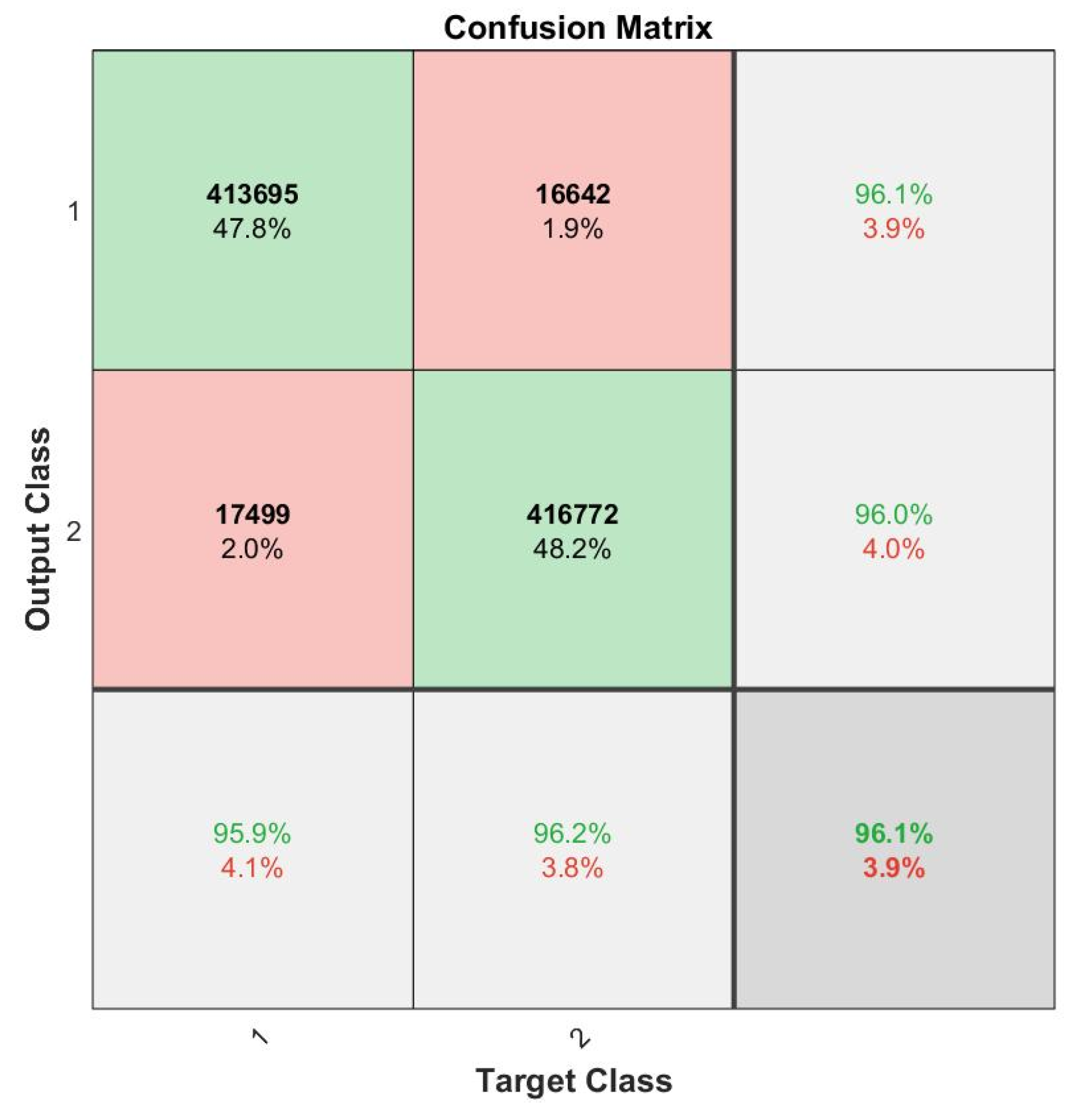
2.3.3. Performance Analysis

To assess the estimation accuracy of the above algorithms, maps are compared to the ones used as ground truth from OSI SAF. In the SIC case, the Mean Absolute Error (MAE) between the daily generated maps and the daily OSI SAF ones is computed. The standard deviation of the error is computed as well. For the SIE case, the quality of the measure is given by the accuracy of the classification. The confusion matrix is also generated, where the accuracy is provided separately for water and ice pixels. In both cases, an error map is generated in which each pixel is computed as the difference between the pixels of the output map and the OSI SAF one. For the MWR maps, the total error will depend on the latitudes where the maps are generated. Latitudes towards the equator will only add more water pixels, and the overall error will be lower. Therefore, MAE is computed in different sets of pixels. One is computed for the global map. The other three are computed regarding the ground truth SIC value. One for all the water pixels, with a SIC of 0%, another one for SIC values above 90%, and the last one for the rest of the SIC values, from 0 to 90%.

Regarding the error for the GNSS-R NNs, it is computed for the whole set of points where there is GNSS-R data and compared to the error of the same specular points without using the GNSS-R data.

3. Results and Discussion

The methodology presented in Section 2 was tested using all the data collected by the FSSCat mission over the first two months of operations, from early October to the end of November 2020. The following subsections present the results regarding different input combinations justifying the selected ones, as well as the final results for the SIC and SIE maps for both poles.

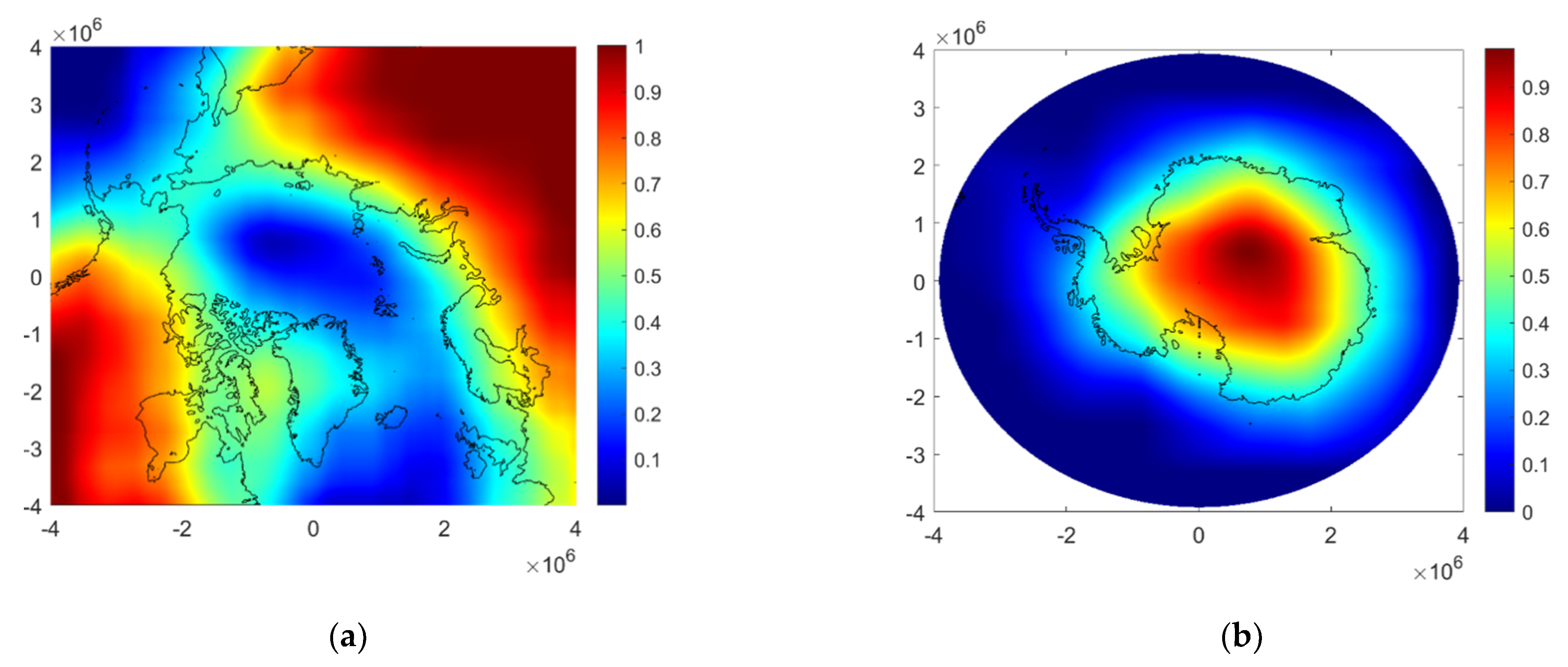
3.1. Neural Network Input Design

The set of optimal input variables was selected in a feature selection step. Different sets of input variables have been used to train and test the NNs in order to evaluate their impact on the SIE classification and the SIC estimation.

Table 1. MWR NN error with respect to the input variables.

		Arctic				Antarctic
		Global	SIC > 90	SIC = 0	0 < SIC < 90	Global	SIC > 90	SIC = 0	0 < SIC < 90
SIE Error	ST	2.12%	0.24%	1.52%	10.58%	14.30%	9.36%	4.52%	34.98%
	ST + LCF	2.07%	0.12%	1.45%	10.54%	12.56%	7.20%	4.74%	30.22%
	MWR	10.61%	1.92%	10.13%	32.05%	5.19%	0.30%	4.58%	10.04%
	MWR + LCF	6.61%	1.18%	5.43%	24.91%	4.46%	0.20%	3.88%	8.74%
	MWR + ST	2.11%	0.06%	1.78%	8.87%	4.16%	0.38%	3.32%	8.51%
	MWR + ST + LCF	1.81%	0.02%	1.52%	8.30%	3.9%	0.20%	2.90%	7.53%
SIC MAE	ST	3.18%	4.08%	4.08%	14.04%	17.02%	14.84%	14.84%	25.19%
	ST + LCF	2.89%	3.60%	1.40%	13.03%	15.78%	13.67%	11.89%	24.13%
	MWR	12.08%	10.06%	10.88%	25.06%	6.90%	6.18%	3.67%	13.02%
	MWR + LCF	7.15%	19.86%	5.93%	19.86%	6.37%	12.46%	3.14%	12.46%
	MWR + ST	2.80%	3.52%	1.32%	13.10%	5.89%	5.73%	2.63%	11.64%
	MWR + ST + LCF	2.37%	2.87%	1.05%	11.27%	5.55%	5.25%	2.35%	11.30%

shows the SIE classification error and the SIC MAE for the different input combinations. As can be seen, the impact of the different variables differs between the Arctic and the Antarctic. On one hand, in the Arctic, the ST by itself possesses most of the information required for generating SIC and SIE maps, while the FMPL-2 MWR by itself does not. On the other hand, in the Antarctic the situation is reversed, the FMPL-2 MWR data are enough to generate SIC and SIE maps with a low error, but the ST data are not. This effect can be explained by the difference in season between the two poles: the melting season for the Antarctic is the freezing season for the Arctic. The higher temperatures at the south pole, as seen in Figure 4, mask the real information about the ice on the surface. During the melting season, water could appear on top of the ice, warming up the surface temperature and misleading the NNs [25]. However, the combination of both measures leads to an improvement in the accuracy of the estimation in all cases, especially in areas with lower SIC, where most of the errors are found.

The selected set of inputs was the last one, including FMPL-2 MWR data and the two auxiliary data sets, ST and LCF. The SIE accuracy of this input set for both poles in areas with SIC concentrations larger than 90% was higher than 99.8%. For areas with intermediate SIC values, the SIE accuracy was 92.5% in the Antarctic and 91.7% in the Arctic, which is a significant improvement compared to the other sets of inputs, especially in the Antarctic. For SIC values, the behavior is the same as for SIE regarding the input variables.

As mentioned previously, the LCF is computed using an averaging box; the size of this box has an impact on the results.

Table 2. MWR NN error with respect to LCF box size.

	Box Size (Pixels)	Arctic				Antarctic
		Global	SIC > 90	SIC = 0	0 < SIC < 90	Global	SIC > 90	SIC = 0	0 < SIC < 90
SIE Error	11 × 11	2.19%	0.06%	1.93%	8.39%	4.05%	0.42%	3.25%	8.25%
	21 × 21	1.99%	0.05%	1.68%	8.37%	3.98%	0.45%	2.91%	8.57%
	51 × 51	2.06%	0.04%	1.75%	8.56%	4.02%	0.33%	3.08%	8.53%
	101 × 101	1.99%	0.03%	1.69%	8.35%	3.97%	0.39%	2.93%	8.55%
	201 × 201	1.95%	0.02%	1.52%	8.50%	3.57%	0.21%	2.90%	7.33%
	301 × 301	2.01%	0.03%	1.67%	8.51%	3.97%	0.31%	3.26%	8.01%
SIC MAE	11 × 11	2.54%	3.14%	1.23%	12.13%	6.01%	5.76%	2.76%	11.83%
	21 × 21	2.42%	2.96%	1.41%	11.75%	5.87%	5.59%	2.58%	11.75%
	51 × 51	2.37%	2.80%	1.15%	11.50%	6.08%	5.66%	2.83%	12.03%
	101 × 101	2.38%	2.86%	1.11%	11.37%	5.86%	5.50%	2.63%	11.72%
	201 × 201	2.37%	2.87%	1.05%	11.27%	5.55%	5.25%	2.35%	11.30%
	301 × 301	2.40%	3.07%	1.10%	11.80%	5.74%	5.36%	2.58%	11.58%

shows the classification error for SIE and the MAE for SIC including both poles. The errors are lower for box sizes close to the antenna footprint. However, notably increasing the size increases the accuracy of the NNs until a minimum error is reached, after which it increases, as does the averaging size. Therefore, an averaging box size of 201 by 201 pixels was chosen to compute the LCF.

LCF improves the results in the zones closer to the coastlines, because it corrects the abrupt temperature changes between land and sea. This can be seen by taking a close look at the results; the LCF has a larger impact on the areas with an SIC larger than 90, or even those with water, because the coastline transitions are usually between land and sea or land and thick ice, where the concentrations are larger. Low concentration areas are usually found between thick ice and sea, where new ice is forming, or the ice is melting.

Regarding the GNSS-R NN, the input selection was performed following a two-step selection procedure. First, the inputs regarding the GNSS-R alone were selected, and then the use of additional sets of data was compared to choose the one with the best performance. Regarding the GNSS-R, the inputs considered were the ADDM, the elevation angle (el), the reflectivity (gamma), the reflectivity standard deviation (STD) and the SNR. Looking at

Table 3. GNSS-R NN error with respect to the input variables (I).

	SIE Classification Error		SIC MAE
	North	South	North	South
DDM	44.90%	46.65%	39.56%	41.31%
ADDM	40.74%	42.10%	37.77%	39.28%
ADDM+ el + gamma + STD	21.61%	13.51%	28.47%	24.32%
ADDM + el + gamma	26.13%	13.42%	31.65%	21.64%
ADDM + el + SNR	26.45%	20.03%	31.77%	29.33%
El + gamma + STD	22.41%	11.77%	27.86%	19.67%
ADDM + el + gamma + STD + SNR	14.91%	6.68%	22.13%	14.69%
El + gamma + STD + SNR	15.73%	9.03%	24.75%	18.29%

, it can be seen, contrary to [4,5], that the DDM by itself is not enough to perform the classification, having an error close to 50%. As mentioned before, the shape of the DDM makes it quite difficult to differentiate between sea and water reflected points, due to its short integration time (40 ms). Nevertheless, after averaging the delay information of the DDM (ADDM), a peak on the center delay bean appears, as shown in Figure 5a. The peak width gives some information about the reflection surface, a bit wider for water reflections than for ice ones. In contrast, averaging the Doppler information of the DDM gives no information to the NN, as shown in Figure 5b. Although SNR and reflectivity are quite similar, using both improves the accuracy of the NNs; they have previously been used together to improve the retrieval of other measures, such as soil moisture [26]. The elevation angle, as expected, improves the classification, because it has a big impact on the received signal. The standard deviation of the reflectivity adds some spatial information to the input [27]; therefore, it improves the results as well.

Finally, the T_b collected by the FMPL-2 MWR and resampled to the GNSS-R resolution also helps with the classification; it is the parameter that has the greatest impact on the results. The combination of the FMPL-2 MWR data and the GNSS-R data is that which gives the best results, showing how the information from MWR is improved thanks to the resolution of GNSS-R.

Table 4. GNSS-R NN error with respect to the input variables (II).

	SIE Classification Error		SIC MAE
	North	South	North	South
GNSS-R	14.91%	6.68%	22.13%	14.69%
GNSS-R + MWR	4.07%	1.60%	10.48%	3.79%
GNSS-R + MWR + LCF	2.36%	1.21%	6.94%	3.44%
MWR	18.04%	6.42%	16.85%	8.14%
MWR + LCF	7.65%	2.59%	10.19%	4.86%
ST	3.44%	40.38%	5.41%	38.09%
ST + LCF	2.51%	20.64%	4.62%	25.74%
MWR + ST	2.20%	3.34%	4.54%	6.63%
MWR + ST + LCF	1.49%	1.85%	3.34%	3.31%
GNSS-R + MWR + LC + ST	1.10%	1.00%	2.81%	2.29%

shows the errors of the NNs with respect to the different data sets used. The GNSS-R dataset includes all the previously selected variables. The MWR, LC and LST datasets are the same ones used for the MWR NNs, but bilinearly interpolated to the specular points of the GNSS-R dataset. As expected, the errors without using de GNSS-R dataset follow the same trends as those presented in Table 1. The classification accuracy for SIE using only the FMPL-2 dataset, i.e., GNSS-R and MWR, is quite good, at 95.9% for the Arctic and 98.4% for the Antarctic. However, using the auxiliary dataset improves it to almost 99% at both poles. For SIC estimation, using all the input datasets, MAE is lower than 3% at both poles. Figure 6 shows the scatter 2D histograms for the last two cases of the table. It can be seen that, for both poles, the GNSS-R corrects the values with larger errors found in the zones with an intermediate SIC value.

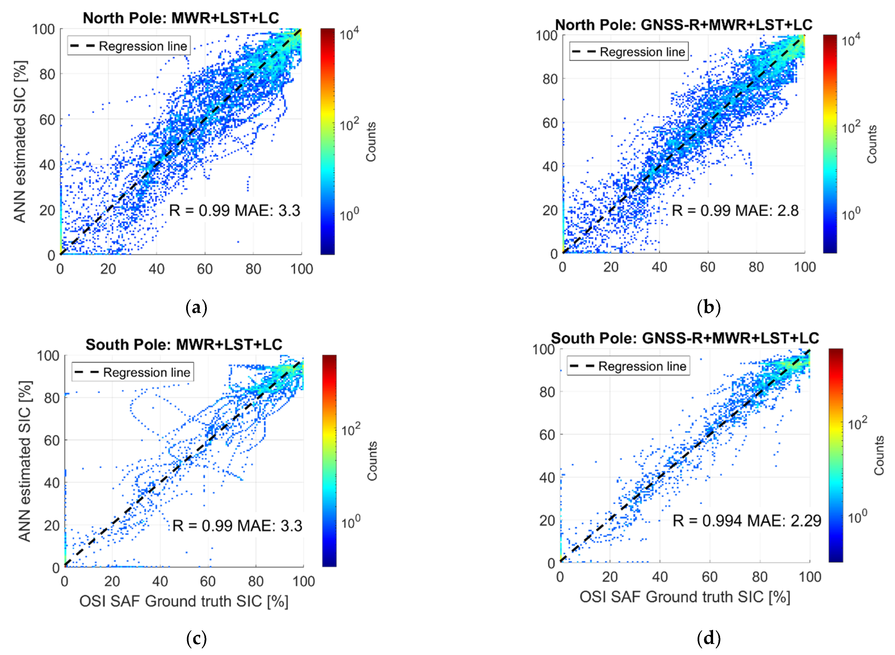
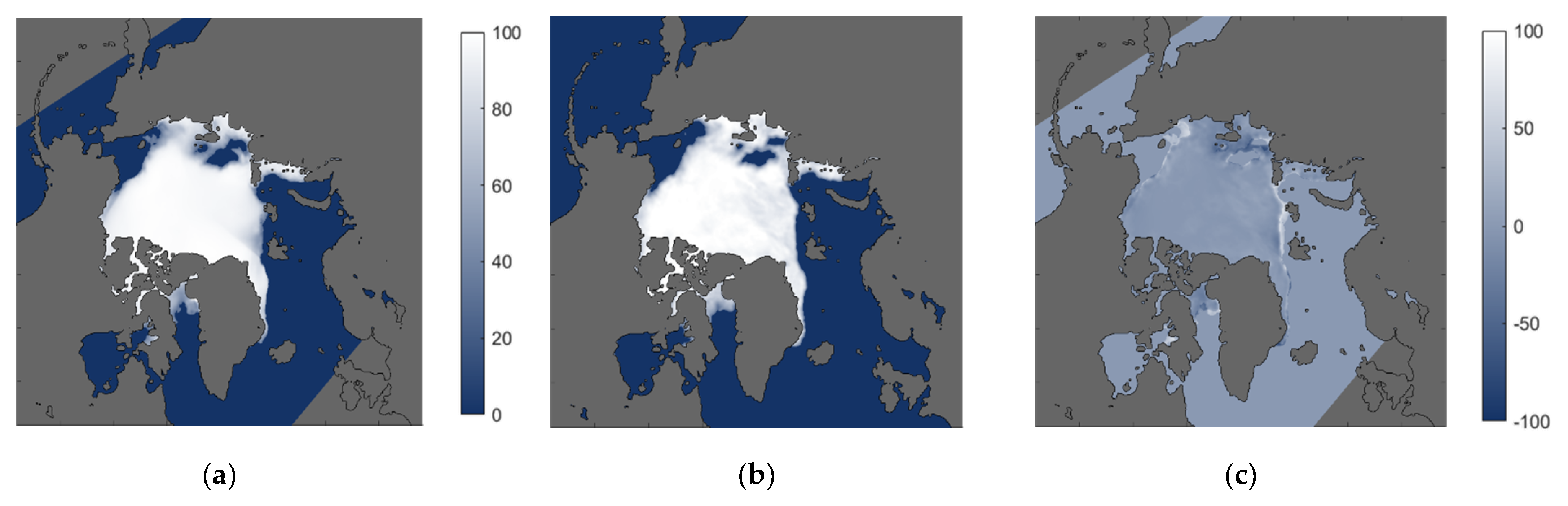
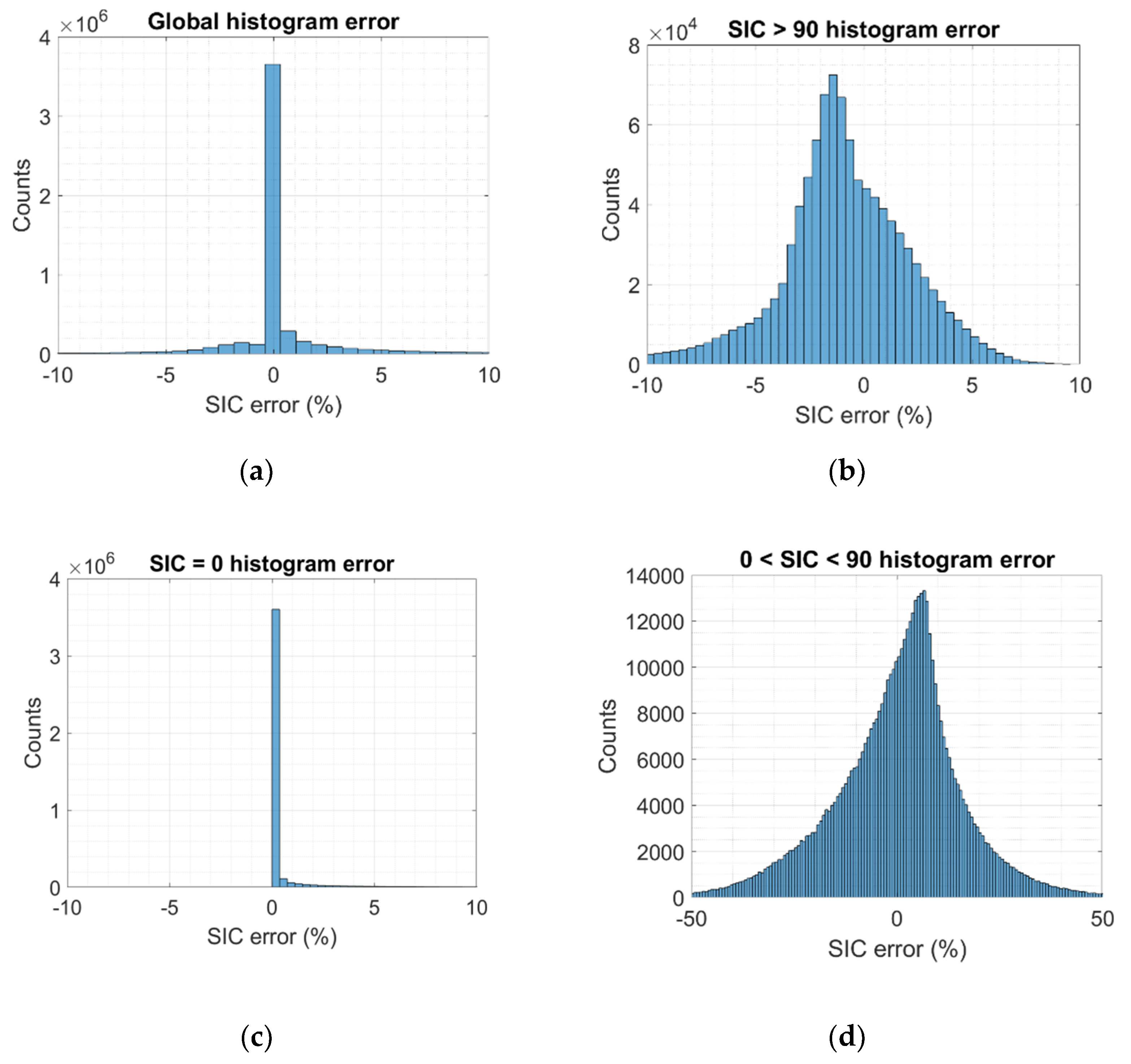
3.2. Sea Ice Concentration Generated Maps

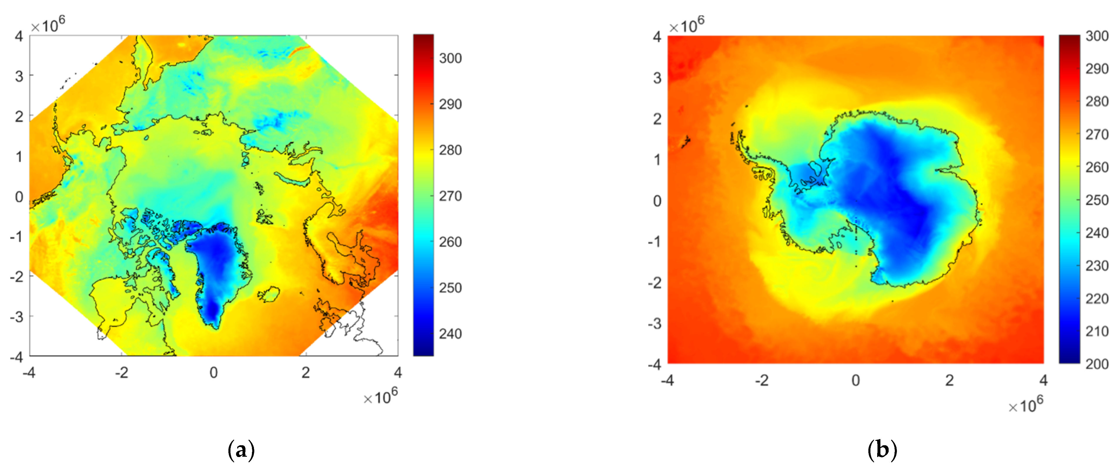
The methodology presented in Section 2 was tested using all the data collected by the FSSCat mission over the first two months of operations, from early October to the end of November 2020. The following subsections present the results for the SIC and SIE maps for both poles.

3.2.1. Arctic Ocean

The first case studied is the SIC retrieval for the Arctic ocean. Daily maps are estimated using the NNs defined in Section 2 and compared to the OSI SAF ones. SIC values are given in percentages. In Figure 7, an SIC map generated using this methodology for the 7 November is presented (Figure 7a), along with the ground truth map (Figure 7b) and the error map (Figure 7c), i.e., the difference between the estimated map and that of the ground truth. An animation with all 44 maps and the error maps generated using FMPL-2 MWR from the Arctic can be seen in Video S1, provided as additional material.

Although the maps are downscaled to 12.5 km, the results are blurred because of the size of the footprint. Therefore, most of the errors accumulate at the transitions between sea and ice, where the SIC is lower. Figure 8 shows the error histogram for each one of the different SIC areas. The results for the North pole SIC maps present a global MAE of 1.95%.

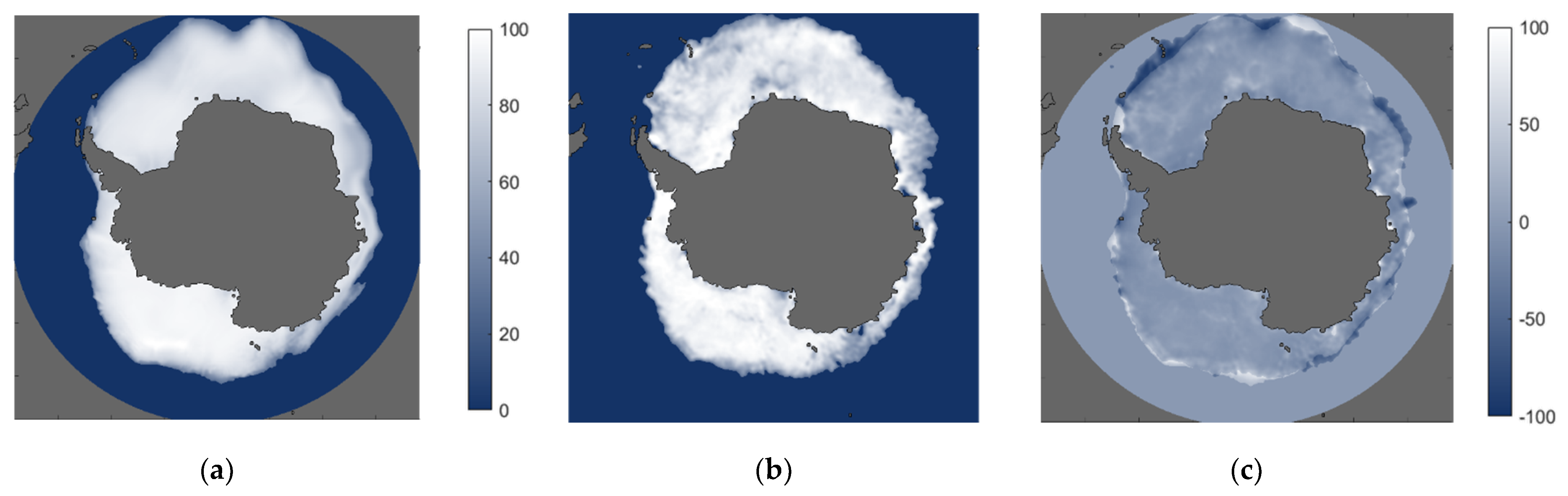
3.2.2. Antarctic Ocean

Regarding the Antarctic ocean, the maps generated are from a three-day period. One of the SIC maps is presented in Figure 9a, corresponding to the period from 13 November to 15 November, along with the ground truth map (Figure 9b) and the associated error map (Figure 9c). As in the north case, an animation with the four maps generated is presented in Video S2 provided as additional material.

In the Antarctic case, the MWR dataset is the one that adds the most information to the NNs. Therefore, the blurry effect due to the footprint of the antenna is more relevant in these maps. The accuracy is worse than in the Arctic ocean due to this effect. For the SIC maps at the South pole, the mean absolute error is 3.57%, the error histograms are shown in Figure 10, with similar results as for the Arctic, but a bit larger, because in the ice mass there are multiple areas with SIC lower than 90%, which are not fully detected due to the antenna footprint.

3.3. Sea Ice Extent Generated Maps

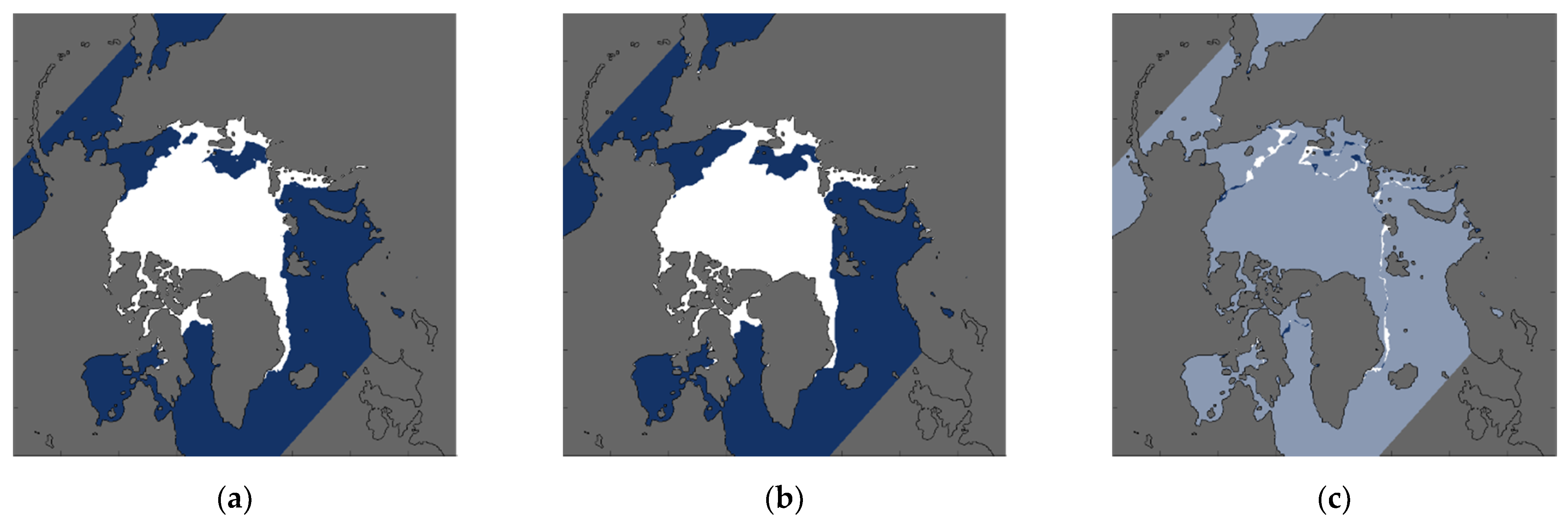
3.3.1. Arctic Ocean

Figure 11 shows an example of the SIE maps generated with the algorithm from the 3 November. The distribution is the same as Figure 7 and Figure 9, showing the SIE map estimated with this methodology (Figure 11a), and the OSI SAF ground truth (Figure 11b), but the color map contains only two values, dark blue for water, and white for ice. Regarding the error maps (Figure 11c), dark blue is for pixels detected as water, but which correspond to ice pixels; light blue means no error; and white is for pixels detected as water, but which correspond to ice. All the SIE maps generated with the algorithm are presented in the Video S3 animation, provided as additional material.

The accuracy for SIE maps of the Arctic is 98.2%, as shown in the confusion matrix in Figure 12; red color shows the error, and green color the accuracy, both in percentage. In the matrix, Class 1 stands for water and Class 2 for ice pixels. As can be seen, errors are again concentrated in the margins of the mass of ice. Furthermore, they are grouped in regions, and are not randomly distributed. The margins of the ice correspond to the areas with lower concentrations, where SIC values change within a small distance from 0% to 100%, and the large footprint of the antenna cannot fully detect those transitions. This error is reduced when there are multiple overpasses, which make it possible to untangle the large footprint size to an extent.

SIE maps make it possible to compute the total area covered by ice at both poles. For the Arctic, the total SIE area is computed from the FMPL-2 maps, and then compared to that from the ground truth maps. As can be seen in Figure 13, each sample corresponds to one day. The mean absolute difference between both algorithms, the present one and the OSI SAF one, is 0.14 million km², which is smaller than the difference between the existing SIE algorithms. As it can be seen in [28] (p. 6) that the differences between existing algorithms are in the range of 1M km². It can be seen that the SIE evolution is very similar to the ground truth.

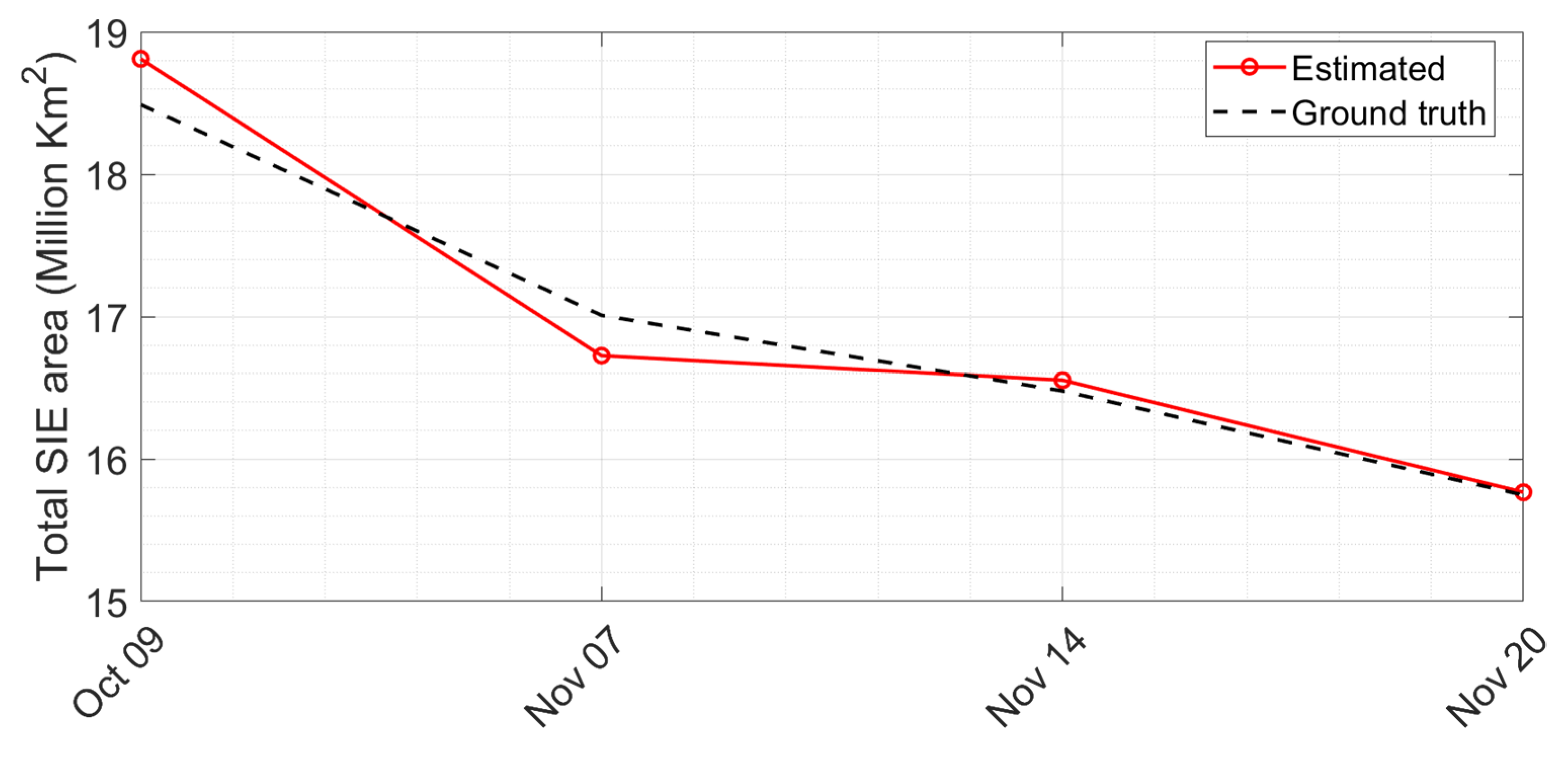
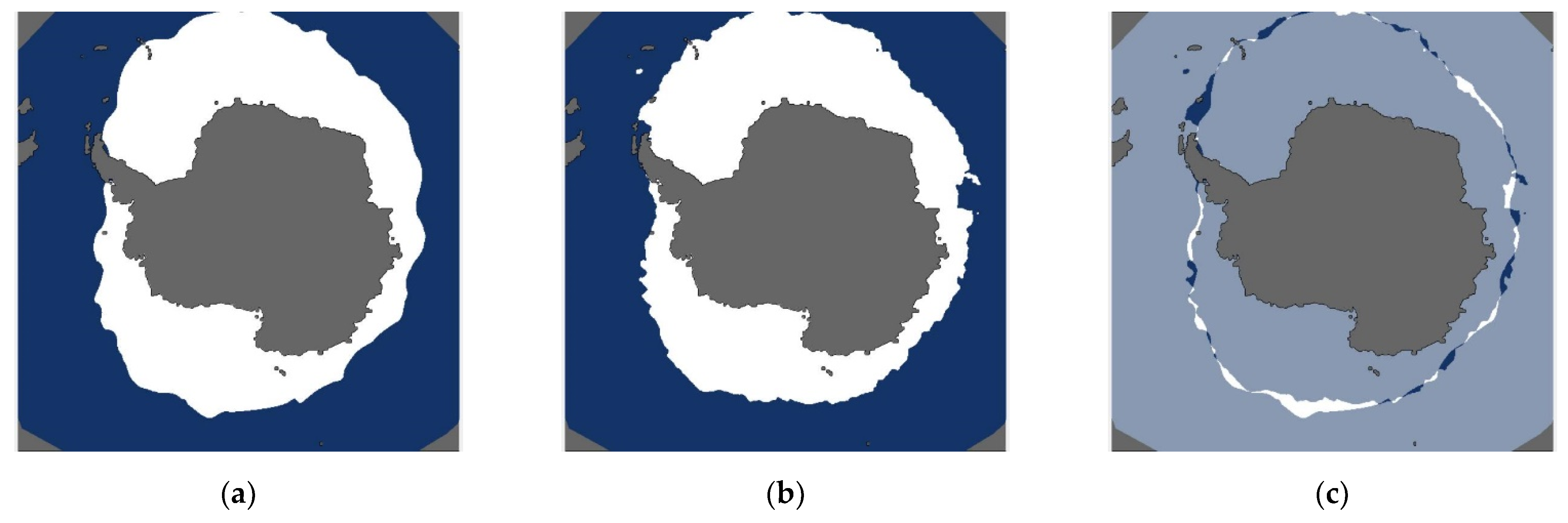
3.3.2. Antarctic Ocean

The computed SIE Antarctic maps are similar to the Arctic ones, but with lower accuracy, for the same reasons as discussed in the SIC section, i.e., the Antarctic is simpler to study than the Arctic. Figure 14 shows the confusion matrix, as before; Class 1 corresponds to water and Class 2 to ice. The accuracy for Antarctica is 96.1%.

The total SIE area from the Antarctic ocean is shown in Figure 15; each data point was computed from one of the generated maps. As before, the difference between the generated maps and the ground truth ones was on the same order of magnitude to that the different SIE retrieval algorithms, with a mean absolute difference of 0.17 million km². Figure 16 shows one of the three-day maps generated using this algorithm for Antarctic; as in the previous section, dark blue represents water, and white represents ice. The effect of the large footprint of the antenna can be seen, as all the errors are grouped along the edges of the ice mass and along the areas with lower presence of sea ice. Video S4, provided as additional material, shows an animation with the four maps generated.

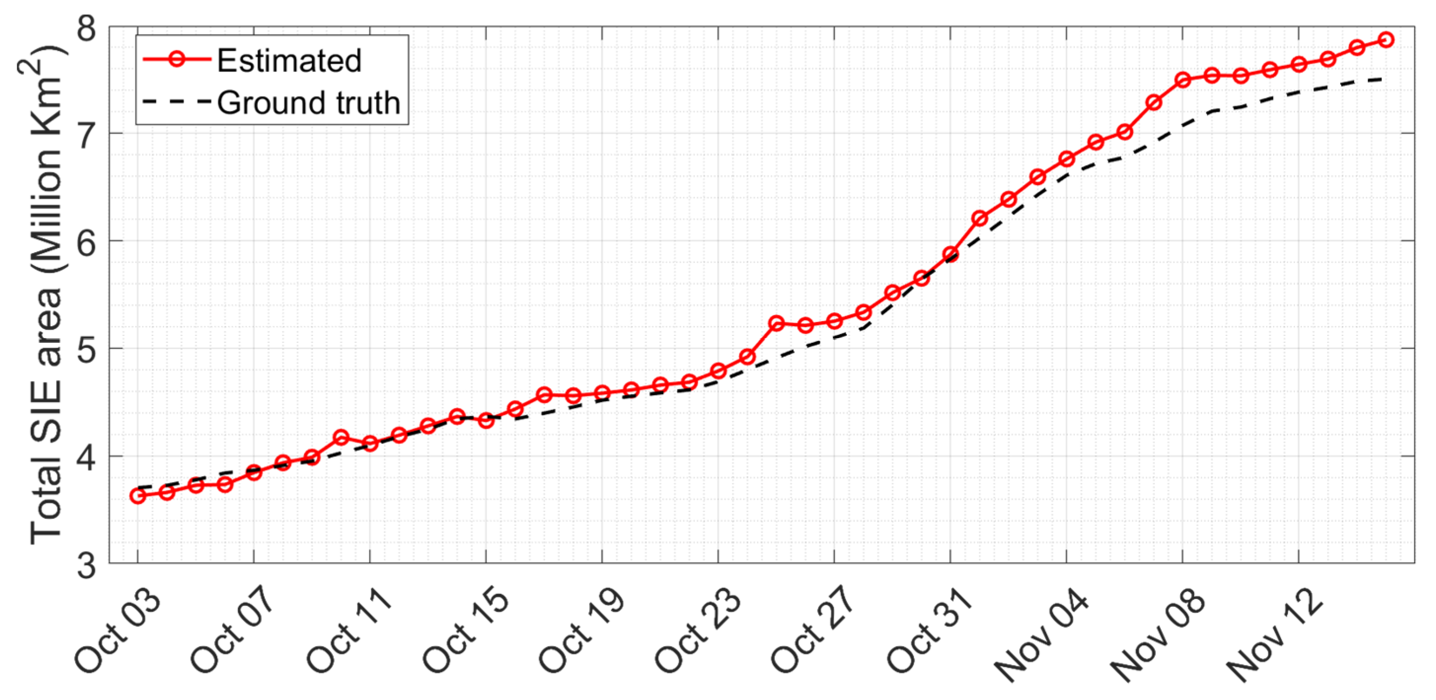
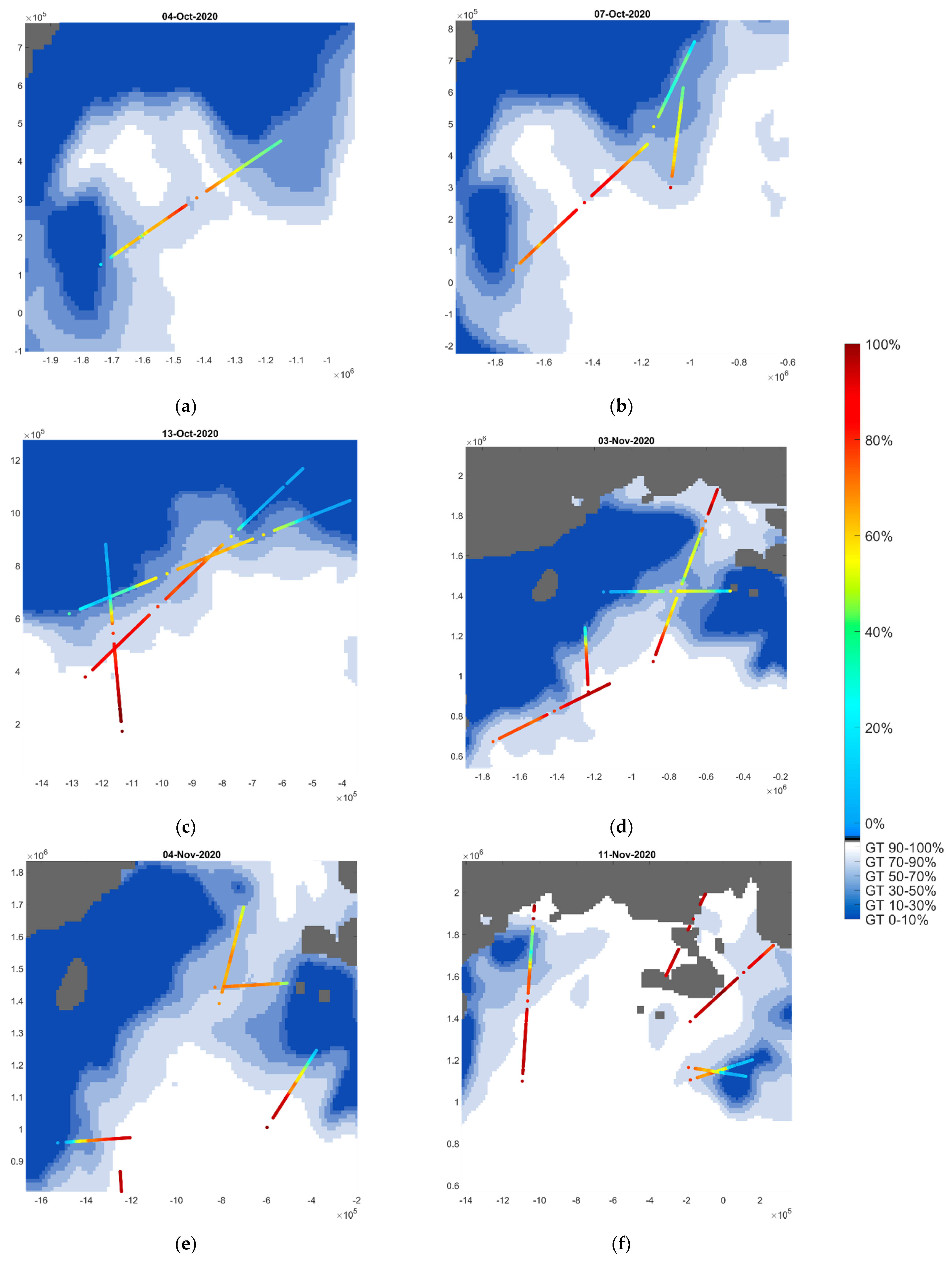
3.3.3. GNSS-R Sea Ice Concentration and Extent Estimation

Once the MWR maps had been generated, the data from the GNSS-R was used to further improve their resolution along the GNSS-R tracks. Classification using the GNSS-R data had an accuracy of 98.9% for the Arctic and 99.0% for the Antarctic. GNSS-R data not only lead to an improvement in the resolution, but also further improve the classification by approximately 1% with respect to the MWR classification. Regarding SIC, MAE is 2.98% for the Arctic and 2.68% for the Antarctic.

GNSS-R data are not presented in full daily maps as MWR data; instead, they are presented by daily tracks. However, with only one satellite carrying GNSS-R, there are only a few tracks per day present, and there are even days without any data. An animation with all the Arctic maps comparing the GNSS-R estimation to the ground truth can be found in Video S5, provided as additional material. To see the GNSS-R SIC estimation clearly, Figure 17 shows six closer looks of the GNSS-R tracks over the OSI SAF ground truth. The ground truth color code shows six levels of SIC. It can be clearly seen in the images that the SIC estimation with the algorithm is really close to the one on the ground truth.

Finally, a composition of the MWR maps and the GNSS-R maps can be seen in Videos S6 and S7, provided as additional material with SIC and SIE, respectively, for the Arctic sea. For Antarctica, the composition was not performed due to the lack of data points available.

4. Conclusions

SIC and SIE maps are currently generated by large satellite missions, carrying microwave radiometers. Today, CubeSats have proved their capabilities for scientific Earth Observation missions at a moderate cost.

FSSCat MWR maps generated with the algorithm presented in this work are resampled at a resolution of 12.5 km, but the blurring due to the real antenna footprint size leads to errors near transitions. However, thanks to the combination of MWR and GNSS-R data, the resolution can be improved along the reflection point tracks to a pixel size of up to 250 m. The GNSS-R resolution is better than the actual products available: 10 km for the OSI SAF products, 4 km for the NSIDC SIC [29] products, and 1 km for the NSIDC SIE [30] products. Thanks to their reduced costs, CubeSats can be launched in large groups for the budget of a single large satellite [31]. A constellation of satellites using both sensors would improve the amount of generated data, and therefore, the quality of the final maps. Furthermore, it will be possible to generate one or more accurate maps with better resolutions in both sensors every day, thanks to the averaging of MWR overlapped data coming from multiple satellites and to the improvement on temporal resolution for GNSS-R. The relationship between the temporal and the spatial resolution in this type of sensors is discussed in [32].

Furthermore, the use of NNs to solve these problems reduces the computational power needed, as shown in other studies [33]. Pre-trained networks would make it possible to perform computations on board, making it necessary only to download the data already processed, thus reducing the data budget required, saving power, and enabling the production of maps in close to real time, a key specification for some use cases. However, NNs need to previously possess accurate maps for training, and this training needs to be done periodically to learn the changing conditions of the sea ice due to climate change. Higher temperatures reduce the proportion of areas with high ice concentrations and increase the areas with intermediate concentrations.

This work presented a methodology for generating SIC and SIE maps using the MWR and GNSS-R data produced by the ³Cat-5/A satellite of the FSSCat mission. The SIC maps were generated with errors lower than 4% for the Antarctic ocean, and even lower for the Arctic ocean (1.8%). Regarding the SIE maps, all of them were generated with an accuracy better than 96.4%. The algorithm uses two different sets of data coming from two sensors, a MWR and a GNSS-R. This makes it possible to generate full coarse-resolution maps quickly with the MWR data and to improve the resolution of these maps using the GNSS-R data on top of them.

References

1. NASA’s Jet Propulsion Laboratory. Global Climate Change, Vital Signs of the Planet. Available online: https://climate.nasa.gov/vital-signs/arctic-sea-ice/ (accessed on 20 February 2021).
2. Thonboe, R.T.; Eastwood, S.; Lavergne, T.; Sørensen, A.M.; Rathmann, N.; Dybkjær, G.; Pederson, L.T.; Høyer, J.L.; Kern, S. The EUMETSAT sea ice concentration climate data record. Cryosphere 2016, 10, 2275–2290. [Google Scholar] [CrossRef] [Green Version]
3. Comiso, J.C.; Cavalieri, D.J.; Parkinson, C.L.; Gloersen, P. Passive microwave algorithms for sea ice concentration: A comparison of two techniques. Remote Sens. Environ. 1997, 60, 357–384. [Google Scholar] [CrossRef]
4. Alonso-Arroyo, A.; Zavorotny, V.U.; Camps, A. Sea Ice Detection Using U.K. TDS-1 GNSS-R Data. IEEE Trans. Geosci. Remote Sens. 2017, 55, 4989–5001. [Google Scholar] [CrossRef] [Green Version]
5. Yan, Q.; Huang, W.; Moloney, C. Neural Networks Based Sea Ice Detection and Concentration Retrieval From GNSS-R Delay-Doppler Maps. IEEE J. Sel. Top. Appl. Earth Obs. Remote Sens. 2017, 10, 3789–3798. [Google Scholar] [CrossRef]
6. Kaleschke, L.; Tian-Kunze, X.; Maaß, N.; Mäkynen, M.; Drusch, M. Sea ice thickness retrieval from SMOS brightness temperatures during the Arctic freeze-up period. Geophys. Res. Lett. 2012, 39, 0094–8276. [Google Scholar] [CrossRef]
7. Selva, D.; Golkar, A.; Korobova, O.; Cruz, I.L.I.; Collopy, P.; de Weck, L. Distributed Earth Satellite Systems: What is needed to move forward. J. Aerosp. Inf. Syst. 2017, 14, 412–438. [Google Scholar] [CrossRef]
8. Planet Labs Inc. Planet. Available online: https://www.planet.com/ (accessed on 1 March 2021).
9. Spire Global. Spire. Available online: https://spire.com/ (accessed on 1 March 2021).
10. Camps, A.; Golkar, A.; Gutierrez, A.; de Azua, J.A.R.; Munoz-Martin, J.F.; Fernandez, L.; Diez, C.; Aguilella, A.; Briatoreet, S.; Akhtyamov, R. FSSCat, the 2017 Copernicus Masters’ “Esa Sentinel Small Satellite Challenge” Winner: A Federated Polar and Soil Moisture Tandem Mission Based on 6U Cubesats. In Proceedings of the IGARSS 2018—2018 IEEE International Geoscience and Remote Sensing Symposium, Valencia, Spain, 22–27 July 2018; pp. 8285–8287. [Google Scholar] [CrossRef]
11. Camps, A.; Muñoz-Martin, J.F.; Ruiz-de-Azúa, J.A.; Fernández, L.; Pérez-Portero, A.; Llavería, D.; Herbert, C.; Pablos, M.; Golkar, A.; Gutiérrrez, A.; et al. FSSCAT Mission Description and First Scientific Results of the FMPL-2 Onboard 3Cat-5/A. In Proceedings of the IGARSS 2021—2021 IEEE International Geoscience and Remote Sensing Symposium, Brussels, Belgium, 12–16 July 2021. submitted. [Google Scholar]
12. Munoz-Martin, J.F.; Capon, L.F.; Ruiz-de-Azua, J.A.; Camps, A. The Flexible Microwave Payload-2: A SDR-Based GNSS-Reflectometer and L-Band Radiometer for CubeSats. IEEE J. Sel. Top. Appl. Earth Obs. Remote Sens. 2020, 13, 1298–1311. [Google Scholar] [CrossRef]
13. Munoz-Martin, J.F.; Fernandez, L.; Perez, A.; Ruiz-de-Azua, J.A.; Park, H.; Camps, A.; Domínguez, B.C.; Pastena, M. In-Orbit Validation of the FMPL-2 Instrument—The GNSS-R and L-Band Microwave Radiometer Payload of the FSSCat Mission. Remote Sens. 2021, 13, 121. [Google Scholar] [CrossRef]
14. Esposito, M.; Vercruyssen, N.; Dijk, C.; Domíguez, B.C.; Pastena, M.; Martimort, P.; Silvestrin, P. HyperScout 2 Highly integration of hyperspectral and thermal infrared technologies for a miniaturized EO imager. Living Planet Symp. 2019. [Google Scholar] [CrossRef]
15. EUMETSAT OSI SAF. Ocean and Sea Ice. Available online: http://www.osi-saf.org/ (accessed on 22 December 2020).
16. Didan, K. “MOD13Q1 MODIS/Terra Vegetation Indices 16-Day L3 Global 250m SIN Grid V006”, NASA EOSDIS Land Processes DAAC. 2015. Available online: https://lpdaac.usgs.gov/products/mod13q1v006/ (accessed on 24 December 2020).
17. Owens, R.; Hewson, T. ECMWF Forecast User Guide; ECMWF: Reading, UK, 2018; Available online: https://www.ecmwf.int/node/16559 (accessed on 24 December 2020).
18. Brodzik, M.J.; Billingsley, B.; Haran, T.; Raup, B.; Savoie, M.H. EASE-Grid 2.0: Incremental but Significant Improvements for Earth-Gridded Data Sets. ISPRS Int. J. Geo-Inf. 2012, 1, 32–45. [Google Scholar] [CrossRef] [Green Version]
19. Zavorotny, V.U.; Gleason, S.; Cardellach, E.; Camps, A. Tutorial on Remote Sensing Using GNSS Bistatic Radar of Opportunity. IEEE Geosci. Remote Sens. 2014, 2, 8–45. [Google Scholar] [CrossRef] [Green Version]
20. Munoz-Martin, J.F.; Perez, A.; Camps, A.; Ribó, S.; Cardellach, E.; Stroeve, J.; Nandan, V.; Itkin, P.; Tonboe, R.; Hendricks, S.; et al. Snow and Ice Thickness Retrievals Using GNSS-R: Preliminary Results of the MOSAiC Experiment. Remote Sens. 2020, 12, 4038. [Google Scholar] [CrossRef]
21. Yan, Q.; Huang, W. Sea Ice Remote Sensing Using GNSS-R: A Review. Remote Sens. 2019, 11, 2565. [Google Scholar] [CrossRef] [Green Version]
22. Schmidhuber, J. Deep learning in neural networks: An overview. Neural Netw. 2015, 61, 85–117. [Google Scholar] [CrossRef] [Green Version]
23. Ying, X. An overview of overfitting and its solutions. J. Phys. Conf. Ser. 2019, 1168, 022022. [Google Scholar] [CrossRef]
24. Yu, H.; Wilamowski, B. Levenberg–Marquardt Training. In Intelligent Systems; CRC Press: Boca Raton, FL, USA, 2011; pp. 1–16. [Google Scholar] [CrossRef]
25. Wait, B.R.; Nokes, R.; Webster-Brown, J. Freeze-thaw dynamics and the implications for stratification and brine geochemistry in meltwater ponds on the McMurdo Ice Shelf, Antarctica. Antarct. Sci. 2009, 21, 243–254. [Google Scholar] [CrossRef]
26. Zribi, M.; Motte, E.; Baghdadi, N.; Baup, F.; Dayau, S.; Fanise, P.; Guyon, D.; Huc, M.; Wigneron, J. Potential Applications of GNSS-R Observations over Agricultural Areas: Results from the GLORI Airborne Campaign. Remote Sens. 2018, 10, 1245. [Google Scholar] [CrossRef] [Green Version]
27. Meier, W.; Stewart, J. Assessing uncertainties in sea ice extent climate indicators. Environ. Res. Lett. 2018, 14, 035005. [Google Scholar] [CrossRef]
28. Fetterer, F.; Stewart, J.S.; Meier, W.N. MASAM2: Daily 4 km Arctic Sea Ice Concentration; Version 1; NSIDC, National Snow and Ice Data Center: Boulder, CO, USA, 2015. [Google Scholar] [CrossRef]
29. Hall, D.K.; Riggs, G.A. MODIS/Terra Sea Ice Extent Daily L3 Global 1km EASE-Grid Day; Version 6; NASA National Snow and Ice Data Center Distributed Active Archive Center: Boulder, CO, USA, 2015. [Google Scholar] [CrossRef]
30. Araguz, C.; Llaveria, D.; Lancheros, E.; Bou-Balust, E.; Camps, A.; Alarcón, E.; Lluch, I.; Matevosyan, H.; Golkar, A.; Tonetti, S.; et al. Optimized model-based design space exploration of distributed multi-orbit multi-platform Earth observation spacecraft architectures. In Proceedings of the 2018 IEEE Aerospace Conference, Big Sky, MT, USA, 3–10 March 2018; pp. 1–16. [Google Scholar] [CrossRef]
31. Bussy-Virat, C.D.; Ruf, C.S.; Ridley, A.J. Relationship Between Temporal and Spatial Resolution for a Constellation of GNSS-R Satellites. IEEE J. Sel. Top. Appl. Earth Obs. Remote Sens. 2019, 12, 16–25. [Google Scholar] [CrossRef]
32. Munoz-Martin, J.F.; Onrubia, R.; Pascual, D.; Park, H.; Pablos, M.; Camps, A.; Rüdiger, C.; Walker, J.; Monerris, A. Single-Pass Soil Moisture Retrieval using GNSS-R at L1 and L5 bands: Results from airbone experiment. Remote Sens. 2021, 13, 797. [Google Scholar] [CrossRef]
33. Krasnopolsky, M.V.; Chalikov, D.V.; Tolman, H.L. A neural network technique to improve computational efficiency of numerical oceanic models. Ocean Model. 2002, 4, 363–383. [Google Scholar] [CrossRef]
Figure 1. FFSCat brightness temperature (K) maps: (a) Arctic, October 7; and (b) Antarctic, 13 November to 15 November.
Remotesensing 13 01139 g001
Figure 2. FMPL-2 GNSS-R data: (a) DDM over water and ice comparison; and (b) Reflectivity tracks over the OSI SAF map.
Remotesensing 13 01139 g002
Figure 3. Land cover fraction maps from: (a) Arctic; and (b) Antarctic.
Remotesensing 13 01139 g003
Figure 4. Skin surface temperature (K) maps from: (a) Arctic, October 3; and (b) Antarctic, October 9.
Remotesensing 13 01139 g004
Figure 5. Averaged DDM: (a) Delay dimension (b) Doppler frequency dimension.
Remotesensing 13 01139 g005
Figure 6. Scatter plots: (a) North pole without GNSS-R data, (b) North pole using GNSS-R data, (c) South pole without GNSS-R data (d) South pole using GNSS-R data.
Remotesensing 13 01139 g006
Figure 7. SIC (%) Arctic maps using MWR data from 7 November. (a) FMPL-2 MWR map, (b) Ground truth map, (c) Error map.
Remotesensing 13 01139 g007
Figure 8. Arctic SIC MWR error histogram: (a) Global, (b) SIC > 90%, (c) SIC = 0 (d) 0 < SIC < 90.
Remotesensing 13 01139 g008
Figure 9. SIC (%) Arctic maps using MWR data from 13 November to 15 November. (a) FMPL-2 MWR map, (b) Ground truth map, (c) Error map.
Remotesensing 13 01139 g009
Figure 10. Arctic SIC MWR error histogram: (a) Global, (b) SIC > 90%, (c) SIC = 0 (d) 0 < SIC < 90.
Remotesensing 13 01139 g010
Figure 11. SIE Arctic composites using MWR data from 3 November. (a) FMPL-2 MWR map, (b) Ground truth map, (c) Error map.
Remotesensing 13 01139 g011
Figure 12. MWR SIE Arctic confusion matrix.
Remotesensing 13 01139 g012
Figure 13. Total Arctic sea ice extent area.
Remotesensing 13 01139 g013
Figure 14. MWR SIE Antarctic confusion matrix.
Remotesensing 13 01139 g014
Figure 15. Total Antarctic sea ice extent area.
Remotesensing 13 01139 g015
Figure 16. SIE Arctic composites using MWR data from 6 November to 8 November. (a) FMPL-2 MWR map, (b) Ground truth map, (c) Error map.
Remotesensing 13 01139 g016
Figure 17. SIC GNSS-R comparison with OSI SAF: (a) 4 October, (b) 7 October, (c) 13 October, (d) 3 November, (e) 4 November, and (f) 11 November.
Remotesensing 13 01139 g017