Abstract
Estimation of the number and geo-location of oil wells is important for policy holders considering their impact on energy resource planning. With the recent development in optical remote sensing, it is possible to identify oil wells from satellite images. Moreover, the recent advancement in deep learning frameworks for object detection in remote sensing makes it possible to automatically detect oil wells from remote sensing images. In this paper, we collected a dataset named Northeast Petroleum University–Oil Well Object Detection Version 1.0 (NEPU–OWOD V1.0) based on high-resolution remote sensing images from Google Earth Imagery. Our database includes 1192 oil wells in 432 images from Daqing City, which has the largest oilfield in China. In this study, we compared nine different state-of-the-art deep learning models based on algorithms for object detection from optical remote sensing images. Experimental results show that the state-of-the-art deep learning models achieve high precision on our collected dataset, which demonstrate the great potential for oil well detection in remote sensing.
1. Introduction
1.1. Background
Oil remains one of the largest energy sources globally despite the fact that renewable energy will be the fastest growing energy, according to BP’s 2019 Energy Outlook [1]. Petroleum production can affect soil and water (e.g., oil spills), which presents potential risks to the environment and public health. The monitoring of the number and geological distribution of oil wells, the status of oil exploitation, and an established energy early warning mechanism are essential, especially to the policy makers in energy resource management. Therefore, it is crucial to build an automatic oil well detection capability in order to address the challenges in oil well resources planning and environment monitoring. Traditional methods for oil well detection includes mainly relying on an on-site survey. Collecting geo-information by conducting surveys of oil wells is impractical and time consuming especially for large scale monitoring. Optical remote sensing techniques can periodically monitor oil wells by obtaining both spatial and temporal information, which show advantages of unrestricted national boundaries and objectivity of observation.
Oil is generally extracted from underground reservoirs based on drilling and pumping approaches. As underground infrastructure of oil wells are not seen, we use the aboveground infrastructure of oil well pump jacks (Figure 1) to detect the oil wells. Pump jacks are small targets in remote sensing, they are generally 6–12 m long, 2–5 m wide, and 5–12 m high, which may slightly vary depending on the model of the pump jack. In a 0.5 m resolution satellite image, a pump jack only has dozens of pixels with a small amount of target information. As can be seen in Figure 1, the land background of oil well pump jacks varies significantly including wetlands, forests, deserts, etc. Moreover, due to the distinctions in the pump jack installation, even the pump jacks of the same model show completely different shape in the images. Furthermore, the surrounding trees and other types of machinery will increase the difficulty in the detection of oil wells.
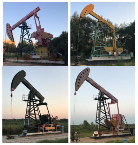
Figure 1.
Sample images of oil well pump jacks onsite images.
In recent years, the development of remote sensing technologies and the rapid improvement in deep learning-based object detection methods make it possible to monitor oil wells from optical remote sensing images. Remote sensing techniques have the advantages of short-term, non-contact, and wide area coverage, repetitive monitoring in earth observation, and are also able to monitor the objects objectively and periodically [2]. Object detection from optical remote sensing images determines objects of interests including vehicles, buildings, airplanes, ships, etc. It also plays a major role in a wide range of applications in environment monitoring and urban planning [3]. The aboveground infrastructure of oil wells shown in Figure 2 have sharp boundaries, which make oil wells independent from background environments; therefore, it is possible to detect oil wells from optical remote sensing images. In addition, the well site and the surrounding facilities of the oil wells, and the road connecting to the well site enable the oil well detection from multiple scales.
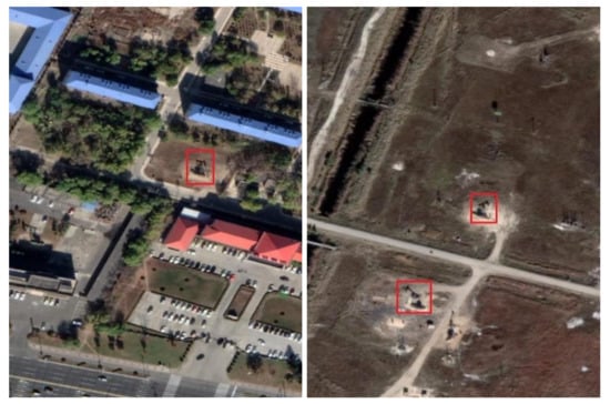
Figure 2.
Sample images of oil well pump jacks from optical remote sensing images (red rectangle boxes show the location of the oil well pump jacks).
Satellite-based remote sensing images are taken from a high-altitude angle of view. There are several challenges in oil well detection. The oil wells are small targets in the remote sensing images (see Figure 3). They are often in the complex backgrounds and different in observation angles, which lead to the uncertainties in remote sensing monitoring and identification. Those challenges in oil well detection from remote sensing images are shown in Figure 3.
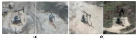
Figure 3.
The challenges in the detection of oil wells from remote sensing images. (a) Oil wells angle differences in remote sensing images. (b) Oil wells background differences in remote sensing images.
1.2. Related Work
1.2.1. Oil-Related Monitoring Using Remote Sensing Techniques
Most of the current relevant studies in the areas of oil-related monitoring are focused on oil spill detection, offshore drilling platforms, and oil tank detection. Oil spill monitoring has been an important topic in the past few decades as it is related to environmental monitoring or disaster monitoring [4,5,6]. For oil spill area detection, a variety of techniques have been used including visible light [7], infrared [8], near-infrared [9], ultraviolet [4], hyperspectral [10], image analysis [11], and satellite radar [12]. In recent years, there has been a significant increase in the research for monitoring of offshore oil resources. Liu et al. [13] used the contextual features extracted from the Defense Meteorological Program/Operational Line-Scan System (DMSP/OLS) night light data. Good recognition results had been achieved on extracting the spatial position information of the South China Sea oil and gas drilling platform by using the time series Landsat-8 Operational Land Imager (OLI) image and layered screening strategy. In recent years, most of the research interests are among the area of remote monitoring of the existing oil tank detection [14] from satellite images. In [15], a traditional machine learning algorithm with the Speeded up Robust Features (SURF) technique and Support Vector Machine (SVM) classifier has been used for oil tank detection. More recently, deep learning-based solutions have been applied in the detection of oil tanks to address the high computational complexity of remote sensing images [16]. In the detection of circular oil storage tanks, a circular support model was established based on the radiological symmetry characteristics of the object, which was verified by GeoEye-1 high-score images [17]. Zhang et al. [18] proposed a recognition algorithm based on deep environment features by using the convolutional neural network (CNN) model and SVM classifier to recognize oil tanks from complex backgrounds and achieved high recognition performance.
Some researchers [19] have used high-resolution satellite images and the Faster regional convolutional neural network (R-CNN) deep learning network (Zhang, Liu et al., 2018) to identify oil facilities and achieved good results. The facilities in well site represents the distribution of oil wells in a certain sense, but the well site can be water injection wells or multiple oil well deployments, which does not represent the true distribution of oil wells. To the best of our knowledge, currently there is no research about the oil well identification based on satellite remote sensing images.
1.2.2. Smart Oilfield
Digital oilfield [20] platform automates the workflow and monitoring the operations in order to reduce the cost and risks. Smart oilfield [21] is a new trend in the oilfield development based on the improvement in the previous digital oilfield. In the last few decades, with the ever-increasing big data, internet of things (IoT), and artificial intelligence (AI), the development of smart oil field has been further enhanced. Different sensors including pressure, density, and temperature sensor have been proposed and deployed to improve the safe and efficient oil pump extraction [22]. Some studies have focused on the exploration and identification of oil wells based on dynamometer card. For example, the electrical parameters from dynamometer card was used for recognition of the working condition of oil wells [23]. Sun et al., used CNN to construct the recognition model of oil well function diagram [24]. The recent remote sensing technologies can be used to remotely monitor the oil wells/oil equipment periodically, which can potentially provide additional data in the area of the smart oilfield.
1.2.3. Deep Learning in Remote Sensing
Recently, with the advancement in the area of optical remote sensing and deep learning algorithms, researchers have been working on detection of various ground targets including the detection of buildings [25,26], ships [27,28,29], airplanes [30,31]. Monitoring oil wells from remote sensing images becomes possible with the advancement of the object detection algorithms based on deep learning frameworks. The hand crafted features were used in traditional machine learning based object detection methods, which are difficult to be applied in massive data scenarios. More recently, a deep learning-based method has replaced the traditional machine learning method by utilizing (more) higher level and deeper features. Training of the deep learning models requires large scales of the dataset, and there are different datasets available for ships, flights and buildings [32,33,34]. In terms of applications related to oil, the detection of oil spills [35,36,37] and oil storage tanks [16] from remote sensing images based on deep learning frameworks received significant attention in recent years. In terms of oil well monitoring, very limited research has been done. Our previous work [38] detected the oil wells from remote sensing images using a Faster regional convolutional neural network (R-CNN) based model, but only a two-stage method has been used.
The use of deep learning based detection methods in remote sensing requires large scale dataset of labeled optical remote sensing images. For example, ImageNet [39], Common Objects in Context (COCO) [40], and pattern analysis, statistical modelling and computational learning (PASCAL) Visual Object Classes (VOC) [41] are widely used publicly available datasets, but none of these datasets provides images for oil wells. To the best of our knowledge, there are no available open oil well satellite image datasets. Therefore, in this work, we construct an oil well dataset from Google Earth Images, which aims to explore the feasibility of automatically detecting and dynamic monitoring of oil wells from remote sensing images. The dataset contains 1192 oil wells in 432 images, which vary in orientation and background. Moreover, we apply different state-of-the-art deep learning frameworks on our dataset to explore the best performance model. Our dataset will be publicly available online [42].
The remaining part of this paper is organized as follows. Section 2 introduces the construction of the dataset. Section 3 describes the state-of-the-art deep learning frameworks, which are used in this work. Section 4 describes the experimental results of applying the state-of-the-art models on our dataset and presents the accuracy of different models. Results are discussed in Section 5, and the conclusion is presented in Section 6.
2. Oil Well Dataset
2.1. Images Collection and Pre-Processing
We constructed a dataset named Northeast Petroleum University–Oil Well Object Detection V1.0 (NEPU-OWOD V1.0) of oil wells that contains the geographical coordinates and labels for each of the oil wells. Our selected research region for this work is in Daqing, China. Daqing is located in North China and is known as “Oil Capital of China”. Our dataset covers an area of 369 square kilometers as seen in Figure 4. The sample images in our dataset are 768 × 768 pixels, 768 × 1024 pixels and 1024 × 1024 pixels. Our dataset contains 432 images which contain 1192 oil wells from Google Earth Images with a very high resolution of 0.41 m per pixel. Figure 5 shows the distribution of the number of oil wells per image. It is noted that in most of the images, there are only 1 or 2 oil wells. In order to increase the diversity of the dataset, we included the images with the different backgrounds and various orientations of the oil wells (see Figure 6).
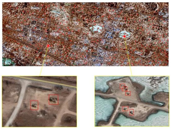
Figure 4.
Map shows the image coverage of Northeast Petroleum University–Oil Well Object Detection V1.0 (NEPU–OWOD) V1.0 dataset.
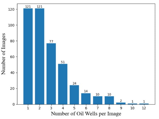
Figure 5.
Distribution of the number of oil wells per image of NEPU–OWOD V1.0 dataset.
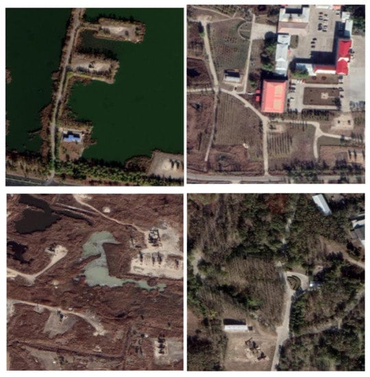
Figure 6.
Sample images from NEPU–OWOD V1.0 dataset.
2.2. Images Annotation/Labeling
The images annotation has been done by local experts and researchers using an open-source annotation tool—RSLabel [43]. Each labeled oil well is saved to an XML file, which includes the geo-location coordinates of the oil wells, images sizes, and bonding boxes sizes, as shown in Figure 7.
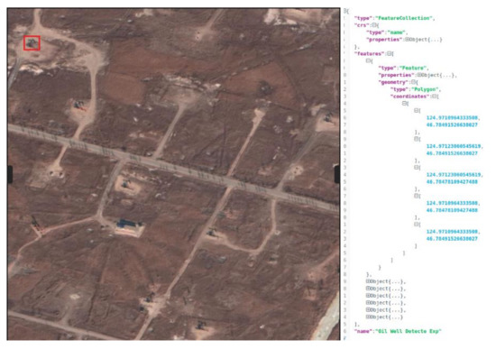
Figure 7.
Oil wells annotation details.
3. Methods
State-of-the-art methods/algorithms: in order to evaluate our dataset, we chosen several state-of-the-art deep learning-based frameworks/models for comparison (see Table 1). In general, the object detection algorithms are divided into two categories, including two-stage method and one-stage method.

Table 1.
State-of-the-art deep learning models used in this work.
3.1. Two-Stage Method
In the area of object detection based on deep learning neural networks, the convolutional neural network (CNN) lays the foundation. The first important approach in the two-stage method is regional convolutional neural network (R-CNN) [44], which initially extracts region proposal and computes features for each proposal based on CNN and then classifies each region. A number of improved approaches have been proposed based on R-CNN which include Fast R-CNN [45] and Faster R-CNN [46]. In this work, we mainly use Faster R-CNN based frameworks which firstly generate several regions of interests by using a Region Proposal Network and then send the proposed regions for object classification and bounding-box regression [47]. It is believed that the two-stage method can achieve higher accuracy rates but are typically slower compared with the one-stage method [48].
3.1.1. Faster R-CNN
In recent years, region proposal methods have been used in most of the object detection applications from the remote sensing images. Based on the first region-based convolutional neural networks (R-CNN) [44], new methods, including Fast R-CNN [45], and Faster R-CNN [46] have been proposed to improve the effectiveness and computation efficiency. As Faster R-CNN is better and faster, we only select Faster R-CNN for the second stage model and it has been used with different backbones (see Table 1). In this work, we used six different backbones for Faster R-CNN. Region Proposal Network (RPN) was proposed by Ren et al. [46] and it has been used in enormous application areas in object detection. For the objects from an input image, RPN is used to generate region proposals and an objectness score for each of the generated proposals. RPN consists of a classifier, which is used to determine the region proposal probability, and a regressor, which is used to regresses the proposal coordinates.
As shown in Figure 8, the deep convolutional networks extract the feature map from the input image, and Faster R-CNN uses convolutional network RPN to generate the region proposals. Then a Region of Interest (ROI) pooling layer is used to converting all the proposals to a fixed shape which is required by the final fully connected layer. ROI takes two inputs, from RPN and feature map, respectively, and flattens and passes them to two fully connected layers. Finally, two fully connected layers are applied to generate a prediction of the target and the best bounding box proposal.
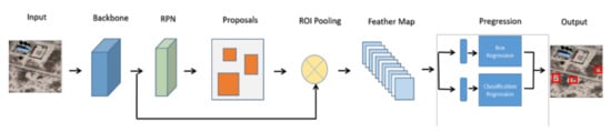
Figure 8.
Faster R-CNN framework.
3.1.2. Backbone Network
Backbone network works as a very important component in CNN based object detection frameworks [49]. In our evaluation, different existing backbone networks e.g., Residual Networks (ResNet) [50], Feature pyramid network (FPN) [51] with ResNet-50 and ResNet-101 have been utilized for feature extraction. In this work, for Faster R-CNN model we selected different combination of backbones including ResNet-50-FPN, ResNet-50-C4, ResNet-50-DC5, ResNet101-FPN, ResNet-101-C4, and ResNet-101-DC5. The evaluation of the performance of Faster R-CNN model with different backbone of oil well detections are presented in Section 4.
3.2. One-Stage Method
One-stage method (or single-stage method) is proposed in recent years to address the challenges in real-time object detection and it predicts straight from image pixels to bounding boxes and class probabilities utilizing only a single deep neural network. The most commonly used one-stage method includes You Only Look Once (YOLO) [52], Single Shot MultiBox Detector (SSD) [53], and RetinaNet [54]. These models usually run much faster compared with the two-stage method.
3.2.1. YOLO
YOLO is the first one-stage method based on convolutional neural network proposed by Redmon et al. [52]. It utilizes a unified architecture and predicts the bounding boxes location and target classification at the same time as a single regression problem by directly extracting the features from input images. Compared with the two-stage method, YOLO is faster. Different versions of YOLO have been proposed, e.g., YOLOv2 and YOLOv3, to improve the detection accuracy and shorten the running time. YOLOv2 [55] is the second version of YOLO and improves YOLO detection performance by incorporating a verity of techniques including batch normalization, high resolution classifier, convolutional with anchor boxes, dimension clusters, direct location predication, fine-grained features, and multi-scale training. YOLOv3 [56] is the third version of YOLO and has made further improvements on YOLO by utilizing a multi-label approach, which better models the data for complex dataset with overlapping labels. Moreover, three different scales were used in YOLOv3 for predicting bounding boxes based on the extracted feature maps and finally the last convolutional layers output three-dimensional (3D) tensor encoding bounding box, objectness, and class prediction. In this work, we used the YOLOv3 framework and the Darknet-53 as the backbone because Darknet-53 is better in detection accuracy and faster than ResNet, according to Redmon and Farhadi’s work [56]. The output predictions have been made at different scales. As in Figure 9, the YOLOv3 employs Darknet-53 as the backbone and then uses Darknet_conv2D_BN_Leaky (DBL) structures. As the basic element of YOLOv3, DBL structure is short for Darknet_conv2D_BN_Leaky which consists of a convolution layer, a batch normalization layer and a leaky ReLU layer [57]. Three different scale feature maps are used in the prediction stage.
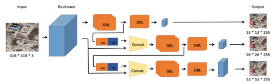
Figure 9.
You Only Look Once (YOLO) v3 framework (with Darknet-53 backbone).
3.2.2. SSD
SSD [53] is another one stage method that has been proposed in 2016 and it is a single-shot detector for multiple categories. It combines a feature extract and detection step based on a feed-forward convolutional network with a non-maximum suppression (NMS). Comparing with the two stage method, SSD removes the generation of the proposal region and incorporates the computation of features in just one stage. Compared with YOLO, SSD model adds several feature layers to the end of a base network [53]. As shown in Figure 10 below, SSD uses VGG16 to extract the feature map through using a Conv4_3 layer and a Pool5 layer. Eight more feature layers have been added after the base network (VGG16) in order to multi-scale feature maps for the detection. The use of multi-scale feature map significantly improves the detection accuracy.
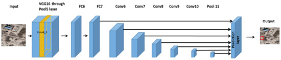
Figure 10.
SSD framework.
3.2.3. RetinaNet
RetinaNet [54] is believed one of the best one-stage methods. It utilizes focal loss for the loss function, which addresses the class imbalance challenges among the one-stage method. The method chosen in this work uses ResNet-50-FPN backbone network as shown in Figure 11. In this framework, ResNet-50 is used to extract deep features. FPN is employed on top of the ResNet backbone to construct rich multi-scale feature pyramid from the input image. The probability of object presence at each spatial position and regresses the offset for bounding boxes are predicted by a classification and box regression subnet which is comprised of a fully convolutional network (FCN) attached to FPN.
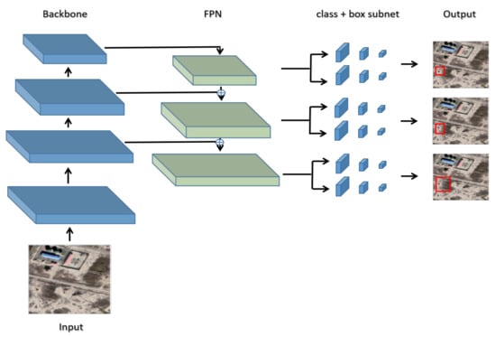
Figure 11.
RetinaNet framework.
4. Experimental Results
4.1. Training Details
In this work, we used our constructed dataset NEPU–OWOD V1.0, which contains 1192 oil wells from Google Earth Images with a very high resolution of 0.41 m per pixel. The size of images in our dataset varies from 768 × 768 pixels, 768 × 1024 pixels and 1024 × 1024 pixels. The training dataset included 345 images with 968 oil wells, which are randomly selected and the remaining is test dataset which included 87 images with 224 oil wells. All of the experiments were carried out on a server with Intel i9-9900KF CPU (3.60 GHz) and a NVIDIA GeForce RTX 2080Ti GPU (11264M).
Training Loss
The training loss changes are present in Figure 12 and Figure 13 for both two-stage methods and one-stage method, respectively. As shown in Figure 12, Faster R-CNN ResNet-101-DC5 (Figure 12d) is more robust with a faster convergence compared with other two-stage frameworks with different backbones used in this work. For one-stage model training loss (Figure 13), RetinaNet converges more quickly and has more robust training loss compared with YOLOv3 and SSD.
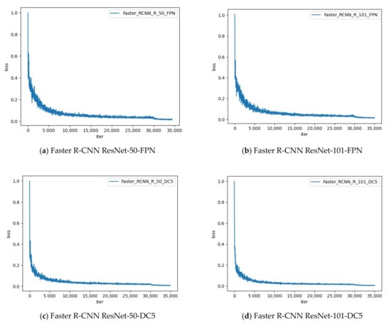
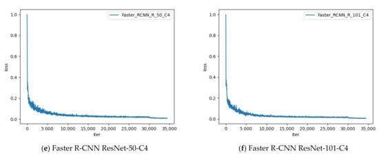
Figure 12.
Training loss for two-stage method models.
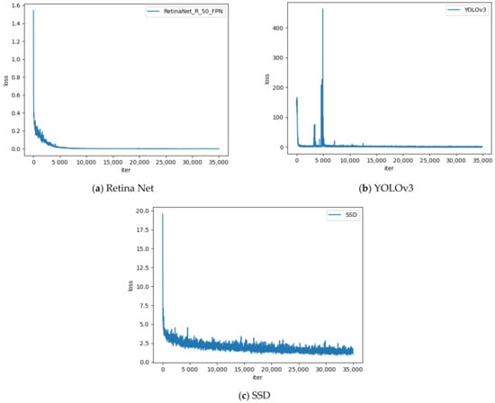
Figure 13.
Training loss for one-stage method models.
4.2. Evaluation Metrics
In this work, we mainly used several metrics, including precision, recall, F1 score, average precision (AP), and receiver operating characteristic (ROC) curve to evaluate different models proposed in Section 3.
4.2.1. Intersection over Union (IoU)
IoU, also known as Jaccard index, is one of the most commonly used evaluation metrics of object detection. IoU is computed as the Equation (1) below, it compares the similarities between the prediction and ground truth area.
where A and B are the prediction and ground truth bounding boxes, respectively. I is intersection Area and U is Union Area.
4.2.2. Precision, Recall, and F1 Score
Typically, we need to set a threshold of IoU to obtain the true positive (TP). When IoU > 0.5, the result is considered as TP.
where TP is true positive, FP is false positive, and FN is false negative.
4.2.3. AP
AP combines recall and precision by computing the average precision over the recall and is defined as the area under the precision–recall curve as in Equation (5) below [58]. In object detection, the performance is usually evaluated by computing AP under different IoU thresholds [49]. AP50 and AP75, referring to the IoU threshold at 50% and 75%, are used, respectively. A higher AP value indicates a better performance.
4.2.4. McNemar’s Test
In order to evaluate if different state-of-art-models are significantly different from each other, McNemar’s test [59] is used. Equation (6) below shows the calculation of McNemar’s test statistic. The p-value threshold of 0.05 is used and the p-value lower than this threshold will indicate a significant difference between the two models.
where b is total number of test instances that the first model gets correct, but the second model gets incorrect, and c is total number of test instances that the first model gets incorrect, but the second model gets correct.
4.2.5. ROC Curve
ROC curve displays the sensitivity (TPR) on y-axis and (1-specitivity) (FPR) on x-axis graphically for varying cut-off points of the test values [60]. The area under the curve (AUC) is an important and effective measure for the performance of a model. A good model has an AUC close to 1, while a poor model has an AUC close to 0. Figure 14 shows the ROC curves for all nine state-of-the-art models used in this study. RetinaNet has the highest AUC (0.86) among all nine state-of-the-art models.
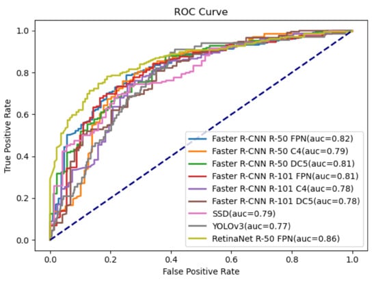
Figure 14.
Receiver operating characteristics (ROC) curve for all the models.
4.3. Experimental Results for State-of-Art Algorithms
4.3.1. Comparisons of Oil Well Detection Accuracy of Different State-of-the-Art Models
We compared nine different deep learning models for oil well detection. The comparison results are summarized in Table 2 and Table 3. The precision, recall and F1 score are presented for all of the deep learning models at IoU = 0.5 in Table 2. The results show that SSD model achieves the best precision with the shortest training time and lowest memory cost. Faster R-CNN with R101-DC5 backbone has the best performance in recall and F1-score. Faster R-CNN and RetinaNet models have relative high recall and F1-score. In Table 3, different AP have been calculated based different deep learning models. RetinaNet model has the best AP and AP50 compared with all the other models and Faster R-CNN with R50-FPN backbone has the best AP75. Figure 15 shows the samples of the detection results.
Table 2.
Oil well detection evaluation metrics (Precision, Recall, and F1 score) (Intersection over Union (IoU) = 0.5). The bold font indicates the best performance.
Table 3.
Oil well detection average precision (AP) of nine state-of-art algorithms. The bold font indicates the best performance.
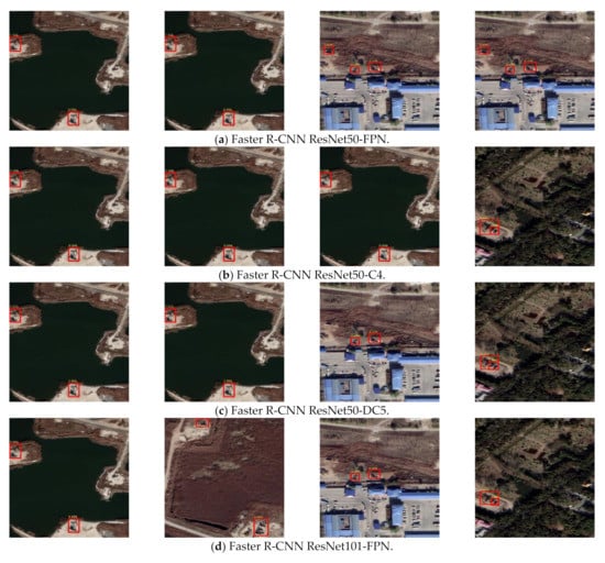
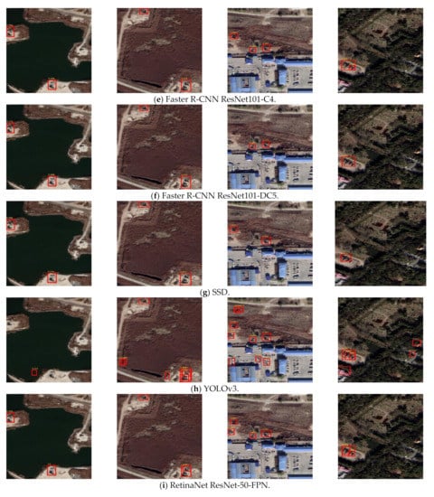
Figure 15.
Object detection results of all the state-of-the-art models. The red boxes represent the detected oil wells.
Table 4 presents the results of McNemar’s Test in order to explore whether the performance differences in different models are significant. Most of the Faster R-CNN models and RetinaNet model are statistically similar while Faster R-CNN ResNet50-DC5, SSD, and YOLOv3 show significantly differences with other models in model performance.
Table 4.
p-value of McNemar’s Test for comparing different deep learning model performances. p-values under 0.05 indicate the two compared models are significantly different. (The bold font indicates models that were statistically different).
4.3.2. Comparisons of Oil Well Detection Accuracy in Different Background and Orientations
In order to further analyze the oil well detection performance under different background and at different orientations, we calculated the precision, recall, and F1-score for each background including bare land, trees, buildings, lakes, and also two different orientations of the oil wells which are horizontal and non-horizontal orientations. Table 5 shows the total number of the oil wells in different backgrounds and orientations in the test dataset. Table 6 shows the performance metrics for each of the background and orientations. It can be seen that the oil well detection accuracy varies with different backgrounds and orientations. The lake background has the best detection performance but there are only 10 images in the test dataset. Bare land background outperforms trees and buildings, which may due to the fact that the trees and buildings are more complicated. In terms of the orientation of the oil wells, it can be seen that the horizontal oil wells are easier to be identified than the non-horizontal oil wells.
Table 5.
Total number of oil wells in the test dataset of different background and orientation.
Table 6.
Oil well detection performance in different backgrounds and orientations (precision, recall, and F1 score (IoU = 0.5)) (The bold font indicates the best performance for each performance metric).
5. Discussion
It is noted that many factors have influences on oil well detection, including the complex backgrounds and differences in observation angles, etc. Therefore, in our dataset, the oil wells in different backgrounds and orientations are included. Oil well clusters will be included in the future to further supplement this dataset.
We trained and tested our dataset on nine different state-of-the-art models, in which six models are two-stage detection models based on Faster R-CNN with various backbones and three models are one-stage detection models based on YOLOv3, SSD, and RetinaNet. The results presented in Section 4 show the SSD achieves the best performance with the highest precision (0.807) and SSD has the lowest training time and lowest memory cost in training. Faster R-CNN R101-DC5 model achieves the best recall (0.928) and F1 score (0.838). To further improve the model performance, we will focus on adjusting the structure of the current nine models to make them achieve better performance for oil well detection.
In the experimental results section, we also compared the model performance of the oil wells in different background and different orientations. For all of the models, the oil wells in the horizontal angle outperform the oil wells in the non-horizontal angle. It is known that the oil wells have the largest shadow when in the horizontal angle, which might work as a more distinguishable feature in training of the model. For oil well detection in all different backgrounds, the two stage model generally has better performance compared with the one stage method. For one stage models, RetinaNet outperforms SSD and YOLOv3 model. It is also noted that the background of lakes and bare land background have better performance than that of the trees and buildings. It may be due to the background of the trees and buildings make the image more complex.
6. Conclusions
In this work, we created an oil well remote sensing image dataset, NEPU–OWOD V1.0, which consists of 1192 oil wells in 432 images collected from Google Earth in Daqing, China. Several state-of-the-art models, including both two-stage methods and one-stage methods, were applied on this dataset. Nine state-of-the-art models were trained and tested on our dataset including Faster R-CNN based frameworks with five different backbones, SSD, YOLOv3, and RetinaNet. The experimental results show that deep learning-based methods are effective in the detection of the oil wells from the remote sensing images. The comparison between different methods and the results show that the deep learning based model is able to detect the oil wells effectively from optical remote sensing images. Moreover, this dataset will provide the opportunity for researchers to develop new object detection algorithms and improve the oil well detection in remote sensing. Researchers will be able to design new oil well detection algorithms utilizing our published dataset.
Author Contributions
Conceptualization, Z.W. and L.B.; methodology, Z.W., L.B., and G.S.; software, G.S.; validation, G.S. and J.Z.; formal analysis, G.S.; investigation, L.B., Z.W. and G.S.; resources, L.B., Z.W., and G.S.; data curation, L.B., Z.W., and G.S.; writing—original draft preparation, Z.W., L.B., G.S., and J.Z.; writing—review and editing, L.B., Z.W., G.S., J.T., M.D.M., R.R.B., and L.C.; visualization, G.S.; supervision, Z.W. and L.B.; project administration, L.C.; funding acquisition, J.T. All authors have read and agreed to the published version of the manuscript.
Funding
This work was supported in part by TUOHAI special project 2020 from Bohai Rim Energy Research Institute of Northeast Petroleum University under Grant HBHZX202002 and project of Excellent and Middle-aged Scientific Research Innovation Team of Northeast Petroleum University under Grant KYCXTD201903.
Institutional Review Board Statement
Not applicable.
Informed Consent Statement
Not applicable.
Data Availability Statement
Publicly available datasets were analyzed in this study. This data can be found here: https://drive.google.com/drive/folders/1bGOAcASCPGKKkyrBDLXK9rx_cekd7a2u?usp=sharing, accessed on 30 December 2020.
Conflicts of Interest
The authors declare no conflict of interest.
References
- BP Energy Outlook. 2019. Available online: https://www.bp.com/content/dam/bp/business-sites/en/global/corporate/pdfs/energy-economics/energy-outlook/bp-energy-outlook-2019-region-insight-global-et.pdf (accessed on 15 December 2020).
- Xue, Y.; Li, Y.; Guang, J.; Zhang, X.; Guo, J. Small satellite remote sensing and applications—History, current and future. Int. J. Remote Sens. 2008, 29, 4339–4372. [Google Scholar] [CrossRef]
- Cheng, G.; Han, J. A survey on object detection in optical remote sensing images. ISPRS J. Photogramm. Remote Sens. 2016, 117, 11–28. [Google Scholar] [CrossRef]
- Fingas, M.; Brown, C. Review of oil spill remote sensing. Mar. Pollut. Bull. 2014, 83, 9–23. [Google Scholar] [CrossRef]
- Fan, J.; Zhang, F.; Zhao, D.; Wang, J. Oil Spill Monitoring Based on SAR Remote Sensing Imagery. Aquat. Procedia 2015, 3, 112–118. [Google Scholar] [CrossRef]
- Jha, M.N.; Levy, J.; Gao, Y. Advances in Remote Sensing for Oil Spill Disaster Management: State-of-the-Art Sensors Technology for Oil Spill Surveillance. Sensors 2008, 8, 236–255. [Google Scholar] [CrossRef]
- Leifer, I.; Lehr, W.J.; Simecek-Beatty, D.; Bradley, E.; Clark, R.; Dennison, P.; Hu, Y.; Matheson, S.; Jones, C.E.; Holt, B.; et al. State of the art satellite and airborne marine oil spill remote sensing: Application to the BP Deepwater Horizon oil spill. Remote Sens. Environ. 2012, 124, 185–209. [Google Scholar] [CrossRef]
- Shih, W.-C.; Andrews, A.B. Infrared contrast of crude-oil-covered water surfaces. Opt. Lett. 2008, 33, 3019–3021. [Google Scholar] [CrossRef] [PubMed]
- Bulgarelli, B.; Djavidnia, S. On MODIS Retrieval of Oil Spill Spectral Properties in the Marine Environment. IEEE Geosci. Remote Sens. Lett. 2011, 9, 398–402. [Google Scholar] [CrossRef]
- Alam, M.S.; Sidike, P. Trends in oil spill detection via hyperspectral imaging. In Proceedings of the 2012 7th International Conference on Electrical and Computer Engineering, Dhaka, Bangladesh, 20–22 December 2012; pp. 858–862. [Google Scholar]
- Bradford, B.N.; Sanchez-Reyes, P.J. Automated oil spill detection with multispectral imagery. SPIE Def. Secur. Sens. 2011, 8030, 80300. [Google Scholar] [CrossRef]
- Fingas, M.; Brown, C.E. A review of oil spill remote sensing. Sensors 2018, 18, 91. [Google Scholar] [CrossRef]
- Liu, Y.; Sun, C.; Yang, Y.; Zhou, M.; Zhan, W.; Cheng, W. Automatic extraction of offshore platforms using time-series Landsat-8 Operational Land Imager data. Remote Sens. Environ. 2016, 175, 73–91. [Google Scholar] [CrossRef]
- Zhang, L.; Liu, C. Oil Tank Detection Using Co-Spatial Residual and Local Gradation Statistic in SAR Images. In Proceedings of the 2019 IEEE International Conference on Image Processing (ICIP), Taipei, Taiwan, 22–25 September 2019; pp. 2000–2004. [Google Scholar]
- Jivane, N.; Soundrapandiyan, R. Enhancement of an Algorithm for Oil Tank Detection in Satellite Images. Int. J. Intell. Eng. Syst. 2017, 10, 218–225. [Google Scholar] [CrossRef]
- Zalpour, M.; Akbarizadeh, G.; Alaei-Sheini, N. A new approach for oil tank detection using deep learning features with control false alarm rate in high-resolution satellite imagery. Int. J. Remote Sens. 2020, 41, 2239–2262. [Google Scholar] [CrossRef]
- Ok, A.O.; Baseski, E. Circular Oil Tank Detection from Panchromatic Satellite Images: A New Automated Approach. IEEE Geosci. Remote Sens. Lett. 2015, 12, 1347–1351. [Google Scholar] [CrossRef]
- Zhang, L.; Shi, Z.; Wu, J. A Hierarchical Oil Tank Detector with Deep Surrounding Features for High-Resolution Optical Satellite Imagery. IEEE J. Sel. Top. Appl. Earth Obs. Remote Sens. 2015, 8, 4895–4909. [Google Scholar] [CrossRef]
- Zhang, N.; Liu, Y.; Zou, L.; Zhao, H.; Dong, W.; Zhou, H.; Zhou, H.; Huang, M. Automatic Recognition of Oil Industry Facilities Based on Deep Learning. In Proceedings of the IGARSS 2018—2018 IEEE International Geoscience and Remote Sensing Symposium, Valencia, Spain, 22–27 July 2018; pp. 2519–2522. [Google Scholar]
- Patri, O.P.; Sorathia, V.S.; Prasanna, V.K. Event-driven information integration for the digital oilfield. In Proceedings of the SPE Annual Technical Conference and Exhibition, San Antonio, TX, USA, 8–10 October 2012. [Google Scholar]
- Ershaghi, I.; Paul, D.; Hauser, M.; Crompton, J.; Sankur, V. CiSoft and smart oilfield technologies. In Proceedings of the Society of Petroleum Engineers—SPE Intelligent Energy International Conference and Exhibition, Aberdeen, UK, 6–8 September 2016. [Google Scholar]
- Hussain, R.F.; Salehi, M.A.; Semiari, O. Serverless Edge Computing for Green Oil and Gas Industry. In Proceedings of the 2019 IEEE Green Technologies Conference, Lafayette, LA, USA, 3–6 April 2019. [Google Scholar]
- Zhuo, J.; Dang, H.; Wu, H.; Pang, H. Pattern Recognition for the Working Condition Diagnosis of Oil Well Based on Electrical Parameters. In Proceedings of the 2018 5th IEEE International Conference on Cloud Computing and Intelligence Systems (CCIS), Nanjing, China, 23–25 November 2018; pp. 557–561. [Google Scholar]
- Sun, L.; Shi, H.; Bai, M. Intelligent oil well identification modelling based on deep learning and neural network. Enterp. Inf. Syst. 2020, 1–15. [Google Scholar] [CrossRef]
- Vakalopoulou, M.; Karantzalos, K.; Komodakis, N.; Paragios, N. Building detection in very high resolution multispectral data with deep learning features. In Proceedings of the 2015 IEEE International Geoscience and Remote Sensing Symposium (IGARSS), Milan, Italy, 26–31 July 2015; pp. 1873–1876. [Google Scholar]
- Prathap, G.; Afanasyev, I. Deep Learning Approach for Building Detection in Satellite Multispectral Imagery. In Proceedings of the 2018 International Conference on Intelligent Systems (IS), Funchal, Portugal, 25–27 September 2018; pp. 461–465. [Google Scholar]
- Yang, X.; Sun, H.; Fu, K.; Yang, J.; Sun, X.; Yan, M.; Guo, Z. Automatic Ship Detection in Remote Sensing Images from Google Earth of Complex Scenes Based on Multiscale Rotation Dense Feature Pyramid Networks. Remote Sens. 2018, 10, 132. [Google Scholar] [CrossRef]
- Li, Q.; Mou, L.; Liu, Q.; Wang, Y.; Zhu, X.X. HSF-Net: Multiscale Deep Feature Embedding for Ship Detection in Optical Remote Sensing Imagery. IEEE Trans. Geosci. Remote Sens. 2018, 56, 7147–7161. [Google Scholar] [CrossRef]
- Lin, H.; Shi, Z.; Zou, Z. Fully Convolutional Network with Task Partitioning for Inshore Ship Detection in Optical Remote Sensing Images. IEEE Geosci. Remote Sens. Lett. 2017, 14, 1665–1669. [Google Scholar] [CrossRef]
- Zhang, F.; Du, B.; Zhang, L.; Xu, M. Weakly Supervised Learning Based on Coupled Convolutional Neural Networks for Aircraft Detection. IEEE Trans. Geosci. Remote Sens. 2016, 54, 5553–5563. [Google Scholar] [CrossRef]
- Fu, K.; Dai, W.; Zhang, Y.; Wang, Z.; Yan, M.; Sun, X. MultiCAM: Multiple Class Activation Mapping for Aircraft Recognition in Remote Sensing Images. Remote Sens. 2019, 11, 544. [Google Scholar] [CrossRef]
- Long, Y.; Gong, Y.; Xiao, Z.; Liu, Q. Accurate Object Localization in Remote Sensing Images Based on Convolutional Neural Networks. IEEE Trans. Geosci. Remote Sens. 2017, 55, 2486–2498. [Google Scholar] [CrossRef]
- Zou, Z.; Shi, Z. Random Access Memories: A New Paradigm for Target Detection in High Resolution Aerial Remote Sensing Images. IEEE Trans. Image Process. 2017, 27, 1100–1111. [Google Scholar] [CrossRef]
- Cheng, G.; Zhou, P.; Han, J. Learning Rotation-Invariant Convolutional Neural Networks for Object Detection in VHR Optical Remote Sensing Images. IEEE Trans. Geosci. Remote Sens. 2016, 54, 7405–7415. [Google Scholar] [CrossRef]
- Chen, G.; Li, Y.; Sun, G.; Zhang, Y. Application of Deep Networks to Oil Spill Detection Using Polarimetric Synthetic Aperture Radar Images. Appl. Sci. 2017, 7, 968. [Google Scholar] [CrossRef]
- Krestenitis, M.; Orfanidis, G.; Ioannidis, K.; Avgerinakis, K.; Vrochidis, S.; Kompatsiaris, I. Oil Spill Identification from Satellite Images Using Deep Neural Networks. Remote Sens. 2019, 11, 1762. [Google Scholar] [CrossRef]
- Jiao, Z.; Jia, C.G.; Cai, C.Y. A new approach to oil spill detection that combines deep learning with unmanned aerial vehicles. Comput. Ind. Eng. 2019, 135, 1300–1311. [Google Scholar] [CrossRef]
- Song, G.; Wang, Z.; Bai, L.; Zhang, J.; Chen, L. Detection of oil wells based on faster R-CNN in optical satellite remote sensing images. SPIE Proc. 2020, 11533. [Google Scholar] [CrossRef]
- Deng, J.; Dong, W.; Socher, R.; Li, L.-J.; Li, K.; Li, F.-F. ImageNet: A large-scale hierarchical image database. In Proceedings of the 2009 IEEE Conference on Computer Vision and Pattern Recognition, Miami, FL, USA, 20–25 June 2009. [Google Scholar]
- Lin, T.-Y.; Maire, M.; Belongie, S.; Bourdev, L.; Girshick, R.; Hays, J.; Perona, P.; Ramanan, D.; Zitnick, C.L.; Dollár, P. Microsoft COCO: Common Objects in Context. In European Conference on Computer Vision; Springer: Cham, Switzerland, 2014; pp. 740–755. [Google Scholar]
- Everingham, M.; Van Gool, L.; Williams, C.K.I.; Winn, J.; Zisserman, A. The Pascal Visual Object Classes (VOC) Challenge. Int. J. Comput. Vis. 2010, 88, 303–338. [Google Scholar] [CrossRef]
- NEPU-OWOD V1.0 (Northeast Petroleum University—Oil Well Object Detection V1.0). Available online: https://drive.google.com/drive/folders/1bGOAcASCPGKKkyrBDLXK9rx_cekd7a2u?usp=sharing (accessed on 28 December 2020).
- RSLabel. Available online: https://github.com/qq2898/RSLabel (accessed on 29 July 2020).
- Girshick, R.; Donahue, J.; Darrell, T.; Malik, J. Rich feature hierarchies for accurate object detection and semantic segmentation. In Proceedings of the IEEE Computer Society Conference on Computer Vision and Pattern Recognition, Columbus, OH, USA, 23–28 June 2014. [Google Scholar]
- Girshick, R. Fast R-CNN. In Proceedings of the 2015 IEEE International Conference on Computer Vision (ICCV), Santiago, Chile, 7–13 December 2015; pp. 1440–1448. [Google Scholar]
- Ren, S.; He, K.; Girshick, R.; Sun, J. Faster R-CNN: Towards real-time object detection with region proposal networks. IEEE Trans. Pattern Anal. Mach. Intell. 2016, 39, 1137–1149. [Google Scholar] [CrossRef]
- Soviany, P.; Ionescu, R.T. Optimizing the Trade-Off between Single-Stage and Two-Stage Deep Object Detectors using Image Difficulty Prediction. In Proceedings of the 2018 20th International Symposium on Symbolic and Numeric Algorithms for Scientific Computing (SYNASC), Timisoara, Romania, 20–23 September 2018; pp. 209–214. [Google Scholar]
- Jiao, L.; Zhang, F.; Liu, F.; Yang, S.; Li, L.; Feng, Z.; Qu, R. A Survey of Deep Learning-Based Object Detection. IEEE Access 2019, 7, 128837–128868. [Google Scholar] [CrossRef]
- Zhao, Z.-Q.; Zheng, P.; Xu, S.-T.; Wu, X. Object Detection with Deep Learning: A Review. IEEE Trans. Neural Netw. Learn. Syst. 2019, 30, 3212–3232. [Google Scholar] [CrossRef]
- Jung, H.; Choi, M.K.; Jung, J.; Lee, J.H.; Kwon, S.; Jung, W.Y. ResNet-Based Vehicle Classification and Localization in Traffic Surveillance Systems. In Proceedings of the IEEE Computer Society Conference on Computer Vision and Pattern Recognition Workshops, Honolulu, HI, USA, 21–26 July 2017. [Google Scholar]
- Lin, T.-Y.; Dollar, P.; Girshick, R.; He, K.; Hariharan, B.; Belongie, S. Feature Pyramid Networks for Object Detection. In Proceedings of the 2017 IEEE Conference on Computer Vision and Pattern Recognition (CVPR), Honolulu, HI, USA, 21–26 July 2017; pp. 936–944. [Google Scholar]
- Uijlings, J.R.R.; Van De Sande, K.E.A.; Gevers, T.; Smeulders, A.W.M. Selective search for object recognition. Int. J. Comput. Vis. 2013, 104, 154–171. [Google Scholar] [CrossRef]
- Liu, W.; Anguelov, D.; Erhan, D.; Szegedy, C.; Reed, S.; Fu, C.Y.; Berg, A.C. SSD: Single shot multibox detector. Comput. Vis. Pattern Recognit. 2016. [Google Scholar] [CrossRef]
- Lin, T.-Y.; Goyal, P.; Girshick, R.B.; He, K.; Dollar, P. Focal Loss for Dense Object Detection. IEEE Trans. Pattern Anal. Mach. Intell. 2020, 42, 318–327. [Google Scholar] [CrossRef] [PubMed]
- Redmon, J.; Farhadi, A. YOLO9000: Better, Faster, Stronger. In Proceedings of the 30th IEEE Conference on Computer Vision and Pattern Recognition, Honolulu, HI, USA, 21–26 July 2017; pp. 6517–6525. [Google Scholar]
- Redmon, J.; Farhadi, A. YOLO v.3. arXiv 2018, arXiv:1804.02767. [Google Scholar]
- Wang, Q.; Bi, S.; Sun, M.; Wang, Y.; Wang, D.; Yang, S. Deep learning approach to peripheral leukocyte recognition. PLoS ONE 2019, 14, e0218808. [Google Scholar] [CrossRef]
- Zhang, E.; Zhang, Y. Average Precision. In Encyclopedia of Database Systems; Metzler, J.B., Ed.; Springer: Boston, MA, USA, 2009; pp. 192–193. [Google Scholar]
- McNemar, Q. Note on the sampling error of the difference between correlated proportions or percentages. Psychometrika 1947, 12, 153–157. [Google Scholar] [CrossRef] [PubMed]
- Kumar, R.; Indrayan, A. Receiver operating characteristic (ROC) curve for medical researchers. Indian Pediatr. 2011, 48, 277–287. [Google Scholar] [CrossRef]


Publisher’s Note: MDPI stays neutral with regard to jurisdictional claims in published maps and institutional affiliations. |
© 2021 by the authors. Licensee MDPI, Basel, Switzerland. This article is an open access article distributed under the terms and conditions of the Creative Commons Attribution (CC BY) license (http://creativecommons.org/licenses/by/4.0/).