
Variational Low-Rank Matrix Factorization with Multi-Patch Collaborative Learning for Hyperspectral Imagery Mixed Denoising


Abstract

1. Introduction
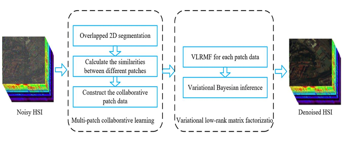
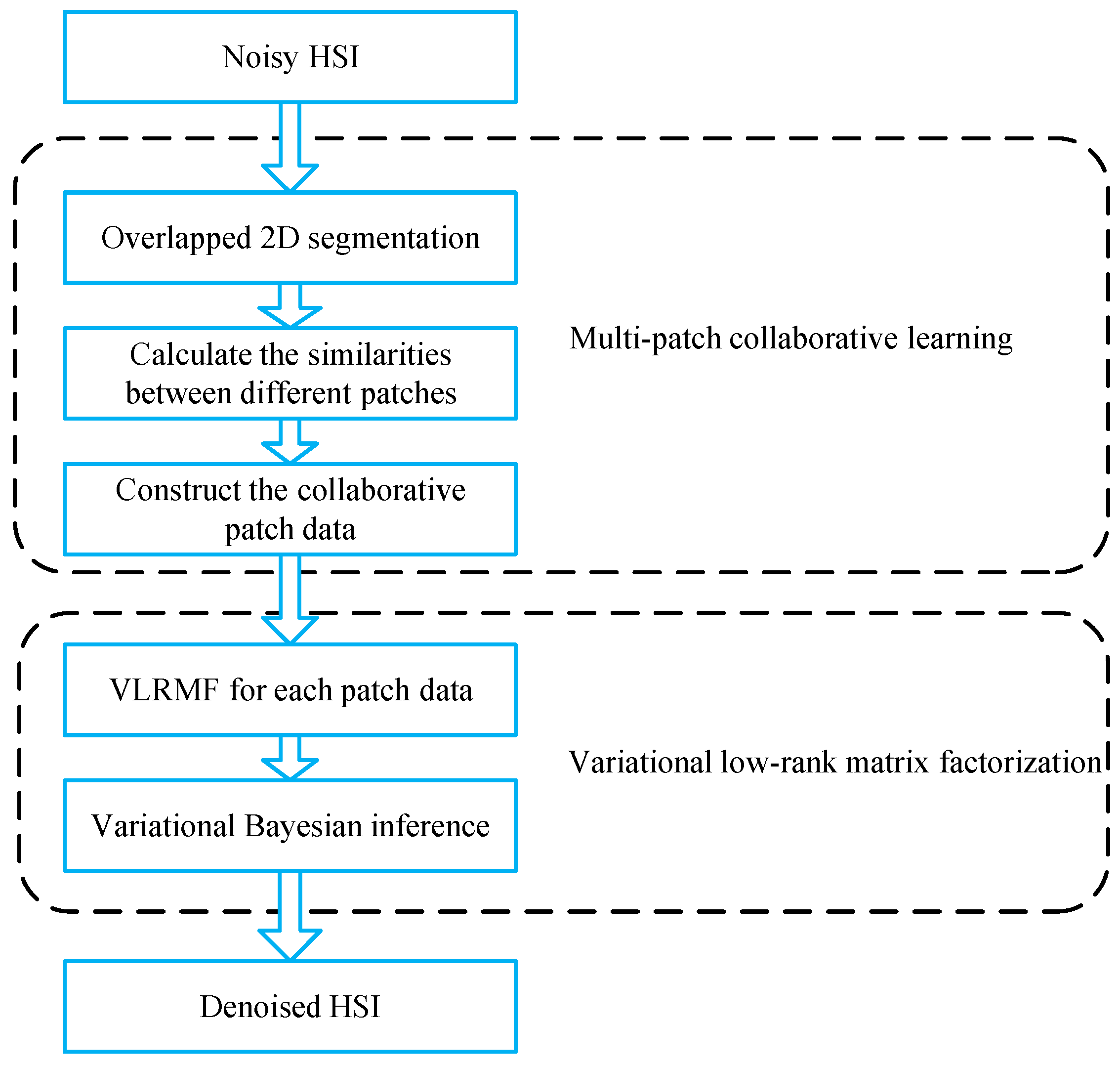
2. Proposed Model
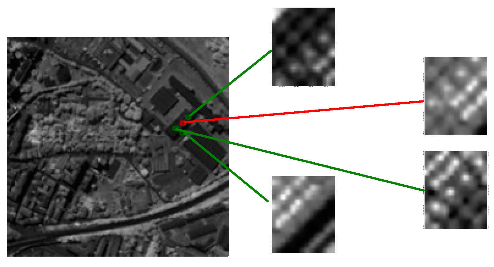
2.1. Multi-Patch Collaborative Learning
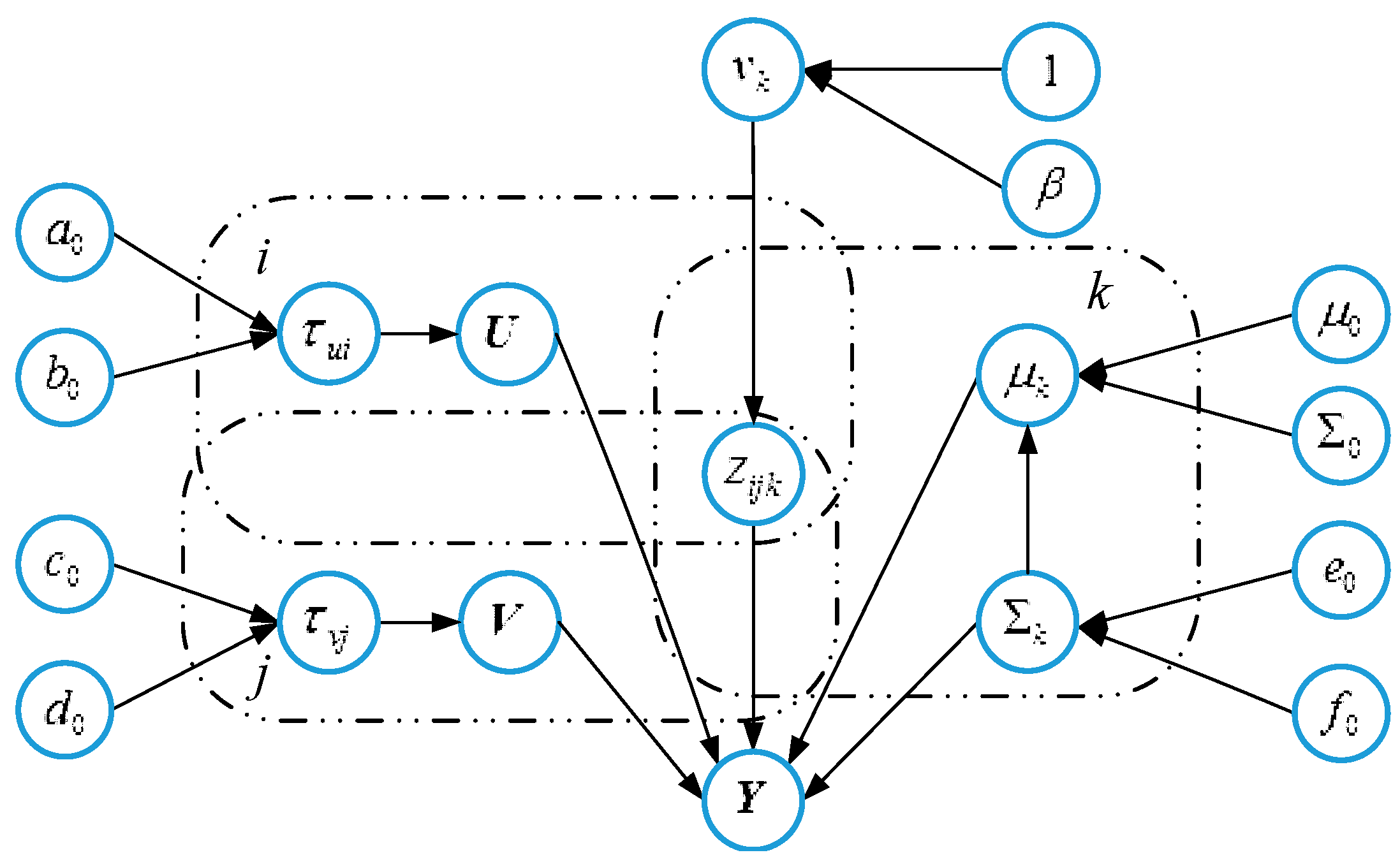
2.2. Variational Low-Rank Matrix Decomposition
2.3. Variational Bayesian Inference
| Algorithm 1. The VLRMFmcl Method |
| Input: the noisy HSI image X; the spatial size of patches; the total number of bands; the hyperparameter ; |
| Output: the denoised image ; |
| Process Source-Code of multi-patch collaborative learning: |
| Divide X into the overlapping patches with the size of ; |
| for each pixel in X do |
| Obtain the collection and , where |
| Calculate the similarities between and ; |
| Select the most similar (P–1) patches to the patch centered at , and construct the collaborative patch data ; |
| Process Source-Code of variational low-rank matrix factorization: |
| Obtain the variables ; |
| Calculate by ; update by minimizing ; |
| return denoised image ; |
3. Experiments
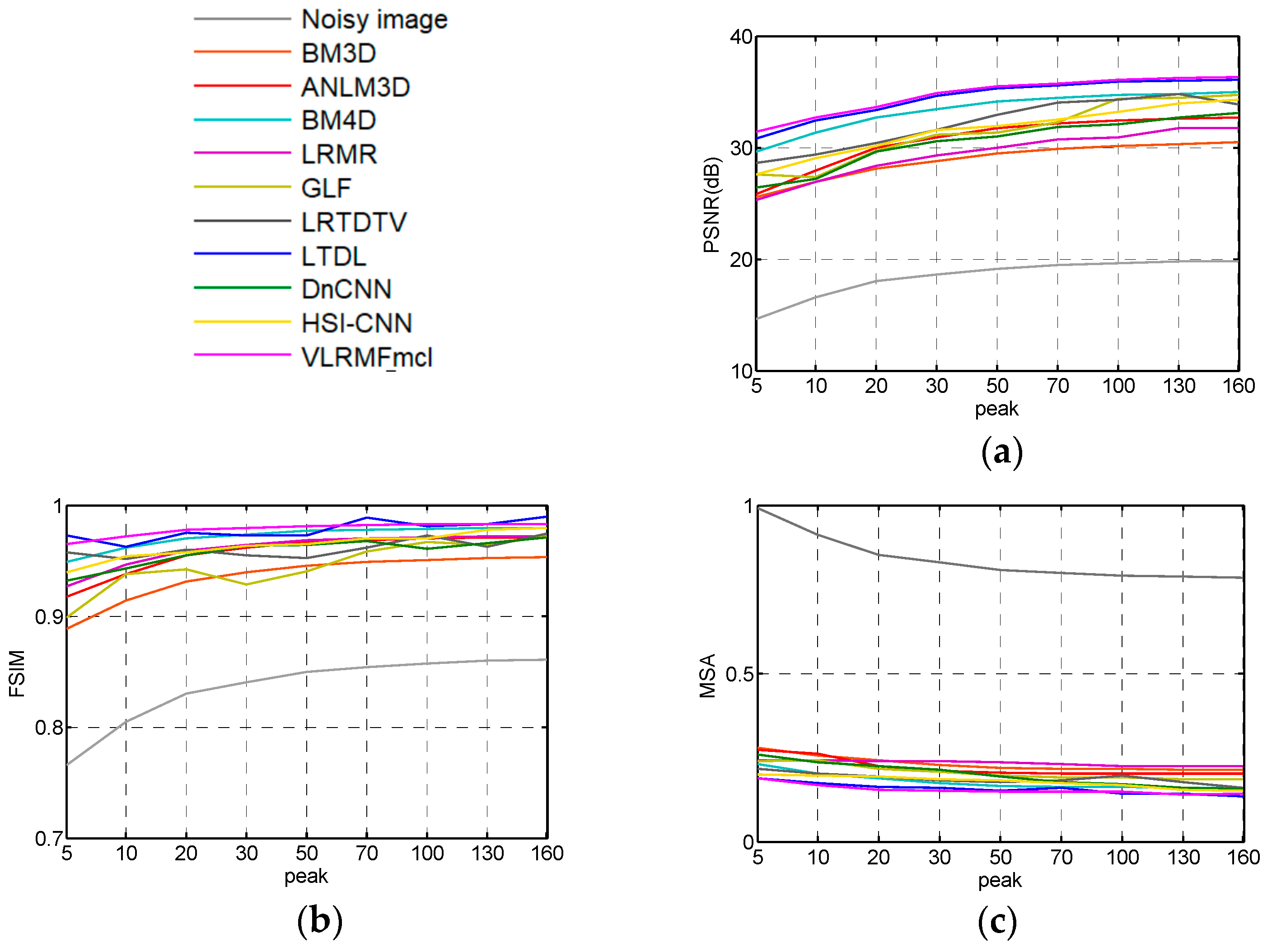
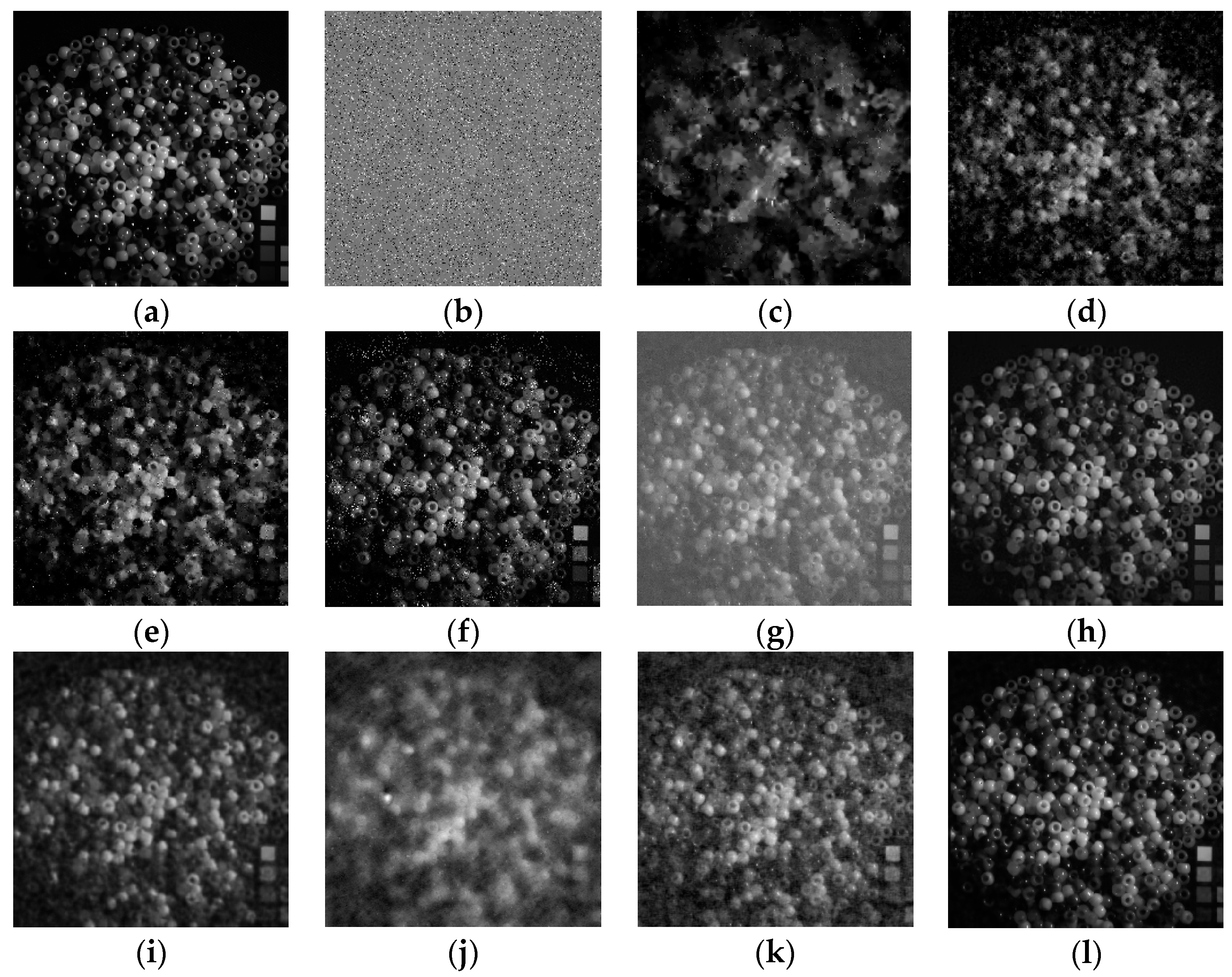
3.1. Experiment on the Beads Data Set
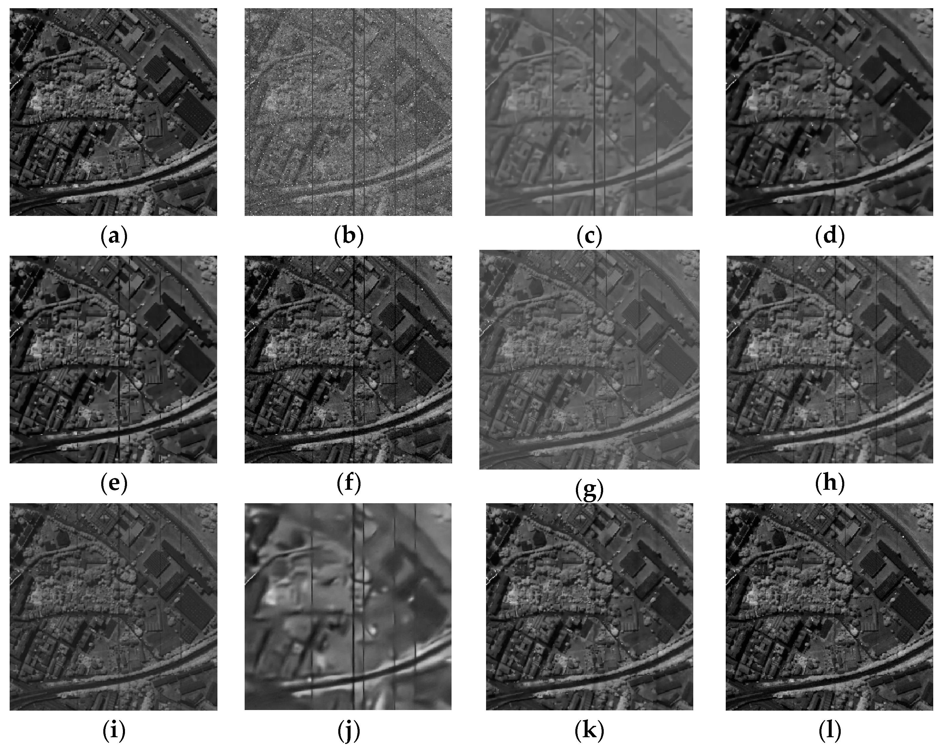
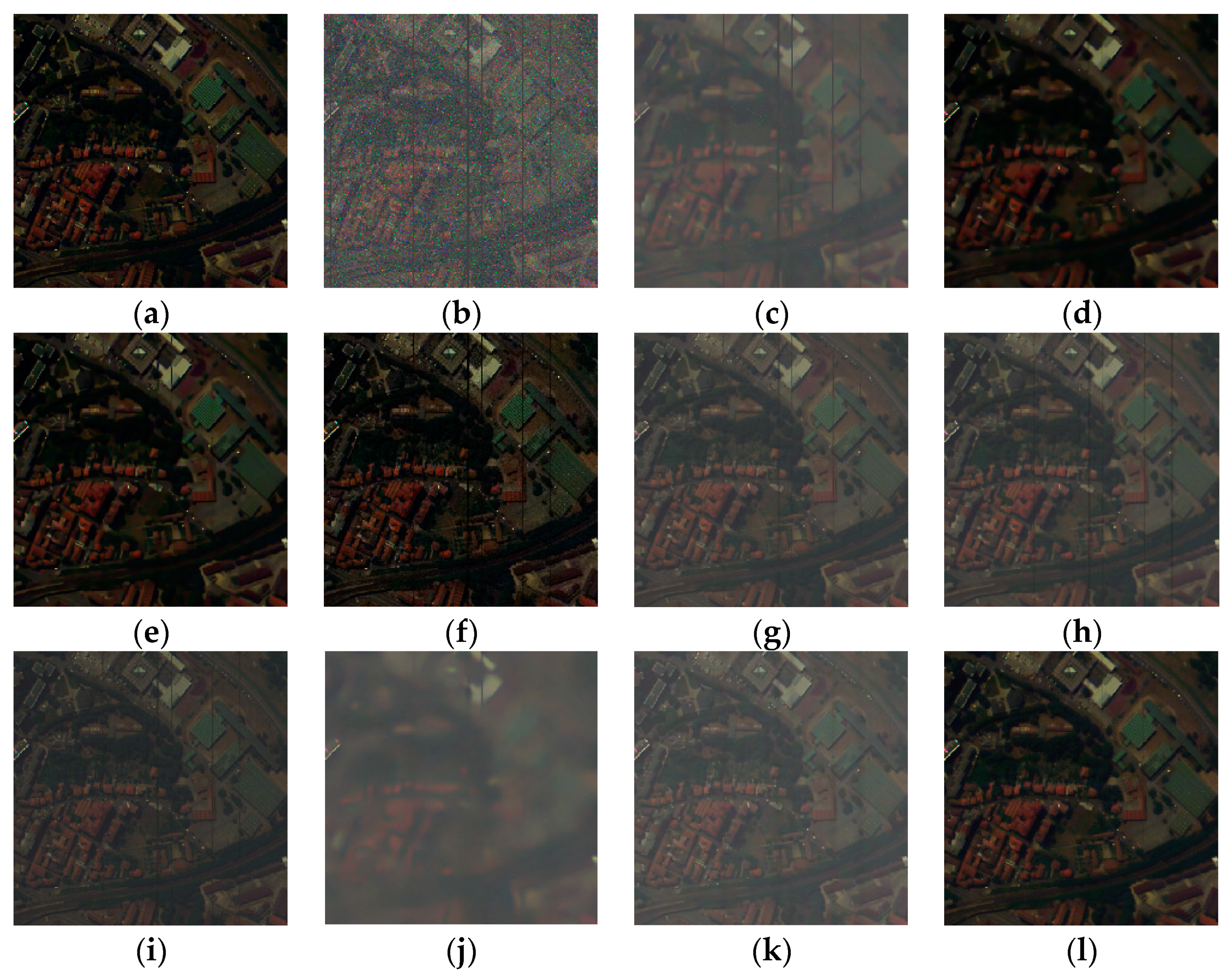
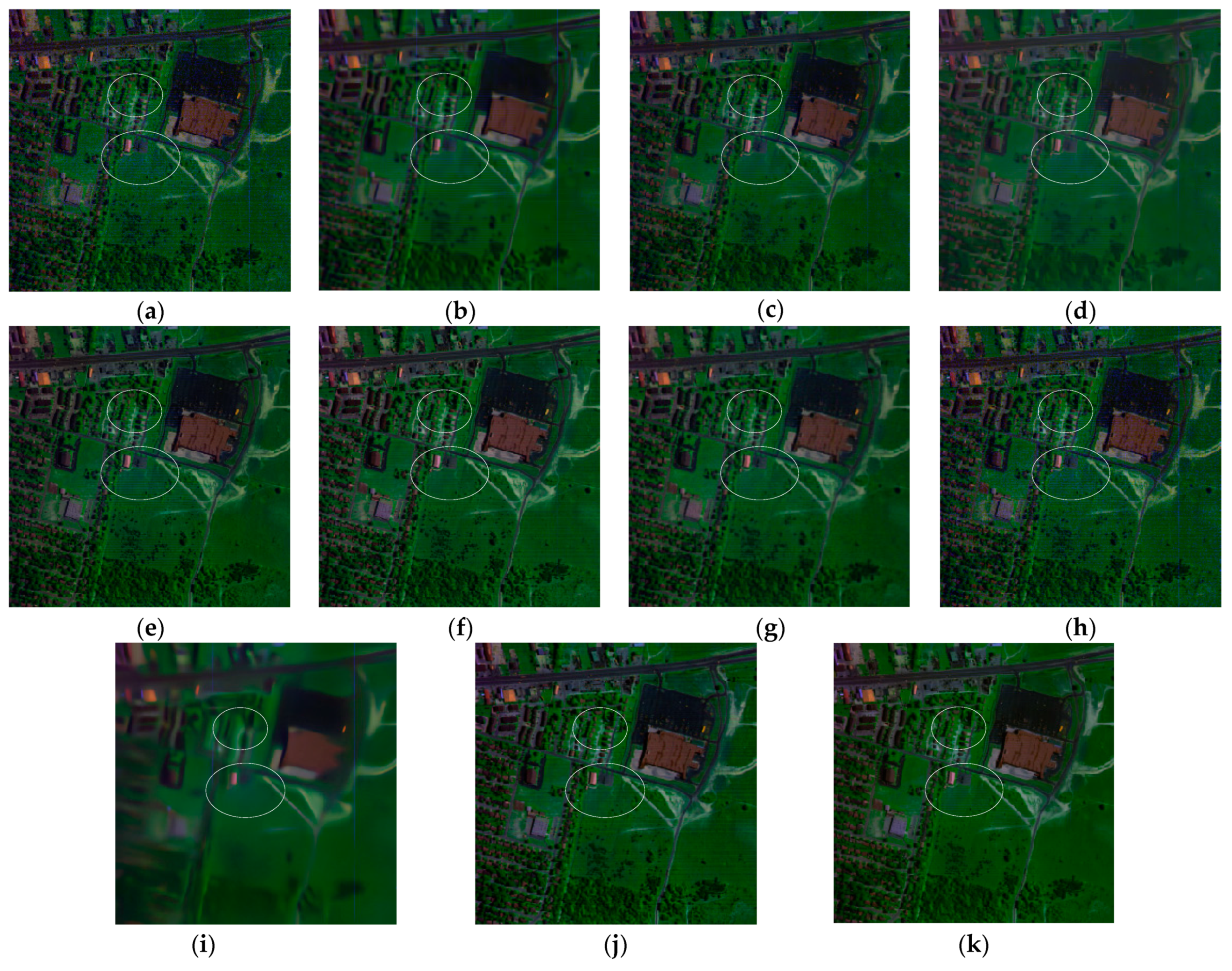
3.2. Experiment on the Pavia Centre Dataset
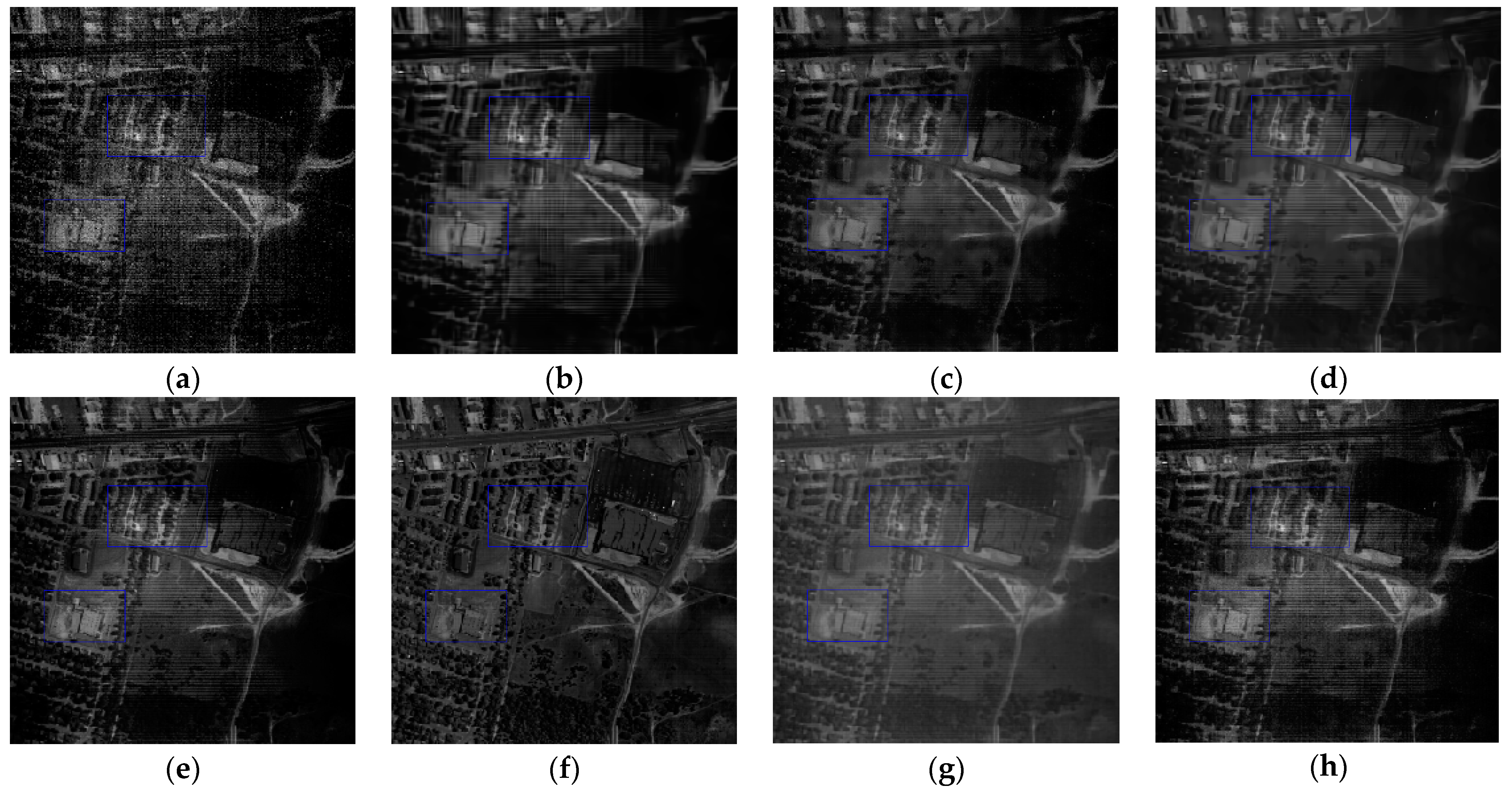
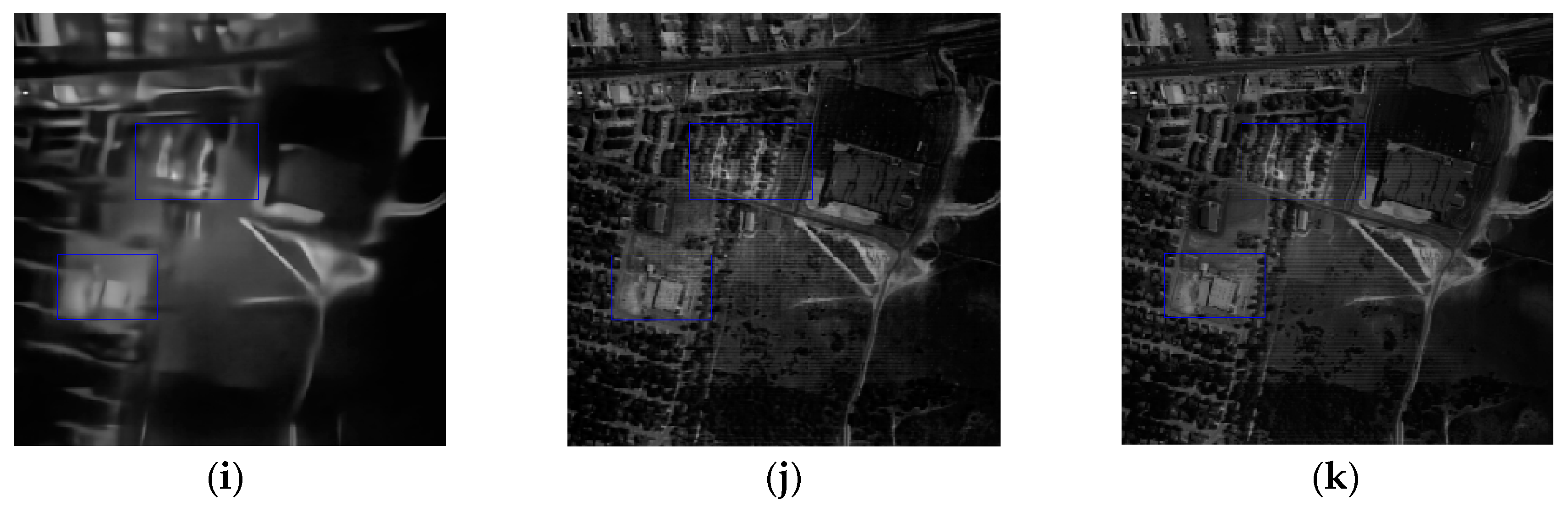
3.3. Experiment on the Urban Dataset
4. Conclusions
Author Contributions
Funding
Institutional Review Board Statement
Informed Consent Statement
Data Availability Statement
Conflicts of Interest
References
- Rasti, B.; Scheunders, P.; Ghamisi, P. Noise reduction in hyperspectral imagery: Overview and application. Remote Sens. 2018, 10, 482. [Google Scholar] [CrossRef]
- Xie, T.; Li, S.; Sun, B. Hyperspectral Images Denoising via Nonconvex Regularized Low-Rank and Sparse Matrix Decomposition. IEEE Trans. Image Process. 2019, 29, 44–56. [Google Scholar] [CrossRef] [PubMed]
- Kong, X.; Zhao, Y.; Xue, J.; Chan, J.C.W.; Ren, Z.; Huang, H.; Zang, J. Hyperspectral image denoising based on nonlocal low-rank and TV regularization. Remote Sens. 2020, 12, 1956. [Google Scholar] [CrossRef]
- Zeng, H.; Xie, X.; Ning, J. Hyperspectral image denoising via global spatial-spectral total variation regularized nonconvex local low-rank tensor approximation. Signal Process. 2021, 178, 107805. [Google Scholar] [CrossRef]
- Lin, B.; Tao, X.; Lu, J. Hyperspectral Image Denoising via Matrix Factorization and Deep Prior Regularization. IEEE Trans. Image Process. 2019, 29, 565–578. [Google Scholar] [CrossRef]
- Sun, L.; Wu, F.; Zhan, T.; Liu, W.; Wang, J.; Jeon, B. Weighted nonlocal low-rank tensor decomposition method for sparse unmixing of hyperspectral images. IEEE J. Sel. Top. Appl. Earth Obs. Remote Sens. 2020, 13, 1174–1188. [Google Scholar] [CrossRef]
- Zhang, S.; Agathos, A.; Li, J. Robust minimum volume simplex analysis for hyperspectral unmixing. IEEE Trans. Geosci. Remote Sens. 2017, 55, 6431–6439. [Google Scholar] [CrossRef]
- Sun, X.; Qu, Y.; Gao, L.; Sun, X.; Qi, H.; Zhang, B.; Shen, T. Target Detection Through Tree-Structured Encoding for Hyperspectral Images. IEEE Trans. Geosci. Remote Sens. 2020. [Google Scholar] [CrossRef]
- Song, X.; Jiang, X.; Gao, J.; Cai, Z. Gaussian Process Graph-Based Discriminant Analysis for Hyperspectral Images Classification. Remote Sens. 2019, 11, 2288. [Google Scholar] [CrossRef]
- Elad, M.; Aharon, M. Image denoising via sparse and redundant representations over learned dictionaries. IEEE Trans. Image Process. 2006, 15, 3736–3745. [Google Scholar] [CrossRef] [PubMed]
- Dabov, K.; Foi, A.; Katkovnik, V. Image denoising by sparse 3-D transform-domain collaborative filtering. IEEE Trans. Image Process. 2007, 16, 2080–2095. [Google Scholar] [CrossRef]
- Othman, H.; Qian, S.-E. Noise reduction of hyperspectral imagery using hybrid spatial-spectral derivative-domain wavelet shrinkage. IEEE Trans. Geosci. Remote Sens. 2006, 44, 397–408. [Google Scholar] [CrossRef]
- Fu, Y.; Lam, A.; Sato, I. Adaptive spatial-spectral dictionary learning for hyperspectral image restoration. Int. J. Comput. Vis. 2017, 122, 228–245. [Google Scholar] [CrossRef]
- Manjn, J.V.; Coup, P.; Mart-Bonmat, L. Adaptive non-local means denoising of MR images with spatially varying noise levels. J. Magn. Reson. Imaging 2010, 31, 192–203. [Google Scholar] [CrossRef] [PubMed]
- Letexier, D.; Bourennane, S. Noise removal from hyperspectral images by multidimensional filtering. IEEE Trans. Geosci. Remote Sens. 2008, 46, 2061–2069. [Google Scholar] [CrossRef]
- Chen, G.; Qian, S.-E. Denoising of hyperspectral imagery using principal component analysis and wavelet shrinkage. IEEE Trans. Geosci. Remote Sens. 2011, 49, 973–980. [Google Scholar] [CrossRef]
- Maggioni, K.E.M.; Katkovnik, V.; Foi, A. Nonlocal transform domain filter for volumetric data denoising and reconstruction. IEEE Trans. Image Process. 2013, 22, 119–133. [Google Scholar] [CrossRef]
- Lu, T.; Li, S.; Fang, L.; Ma, Y.; Benediktsson, J.A. Spectral–spatial adaptive sparse representation for hyperspectral image denoising. IEEE Trans. Geosci. Remote Sens. 2015, 54, 373–385. [Google Scholar] [CrossRef]
- Zhao, L.; Xu, Y.; Wei, Z. Hyperspectral Image Denoising via Coupled Spectral-Spatial Tensor Representation. IEEE Int. Geosci. Remote Sens. Symp. 2018, 4784–4787. [Google Scholar]
- Chen, Y.; He, W.; Yokoya, N.; Huang, T.Z. Hyperspectral image restoration using weighted group sparsity-regularized low-rank tensor decomposition. IEEE Trans. Cybern. 2019, 50, 3556–3570. [Google Scholar] [CrossRef] [PubMed]
- Sun, L.; Jeon, B.; Zheng, Y.; Wu, Z. Hyperspectral image restoration using low-rank representation on spectral difference image. IEEE Geosci. Remote Sens. Lett. 2017, 14, 1151–1155. [Google Scholar] [CrossRef]
- Fan, H.; Chen, Y.; Guo, Y.; Zhang, H.; Kuang, G. Hyperspectral image restoration using low-rank tensor recovery. IEEE J. Sel. Top. Appl. Earth Obs. Remote Sens. 2017, 10, 4589–4604. [Google Scholar] [CrossRef]
- Chen, Y.; Guo, Y.; Wang, Y.; Wang, D.; Peng, C.; He, G. Denoising of hyperspectral images using nonconvex low rank matrix approximation. IEEE Trans. Geosci. Remote Sens. 2017, 55, 5366–5380. [Google Scholar] [CrossRef]
- Okatani, T.; Yoshida, T.; Deguchi, K. Efficient algorithm for low-rank matrix factorization with missing components and performance comparison of latest algorithms. IEEE ICCV 2011, 842–849. [Google Scholar]
- Zhang, H.; He, W.; Zhang, L. Hyperspectral image restoration using low-rank matrix recovery. IEEE Trans. Geosci. Remote Sens. 2014, 52, 4729–4743. [Google Scholar] [CrossRef]
- Zhuang, L.; Bioucas-Dias, J.M. Hyperspectral image denoising based on global and non-local low-rank factorizations. In Proceedings of the 2017 IEEE International Conference on Image Processing (ICIP), Beijing, China, 17–20 September 2017; pp. 1900–1904. [Google Scholar]
- Xue, J.; Zhao, Y.; Liao, W.; Kong, S.G. Joint spatial and spectral low-rank regularization for hyperspectral image denoising. IEEE Trans. Geosci. Remote Sens. 2017, 56, 1940–1958. [Google Scholar] [CrossRef]
- Fan, H.; Li, C.; Guo, Y.; Kuang, G.; Ma, J. Spatial–spectral total variation regularized low-rank tensor decomposition for hyperspectral image denoising. IEEE Trans. Geosci. Remote Sens. 2018, 56, 6196–6213. [Google Scholar] [CrossRef]
- Wang, Q.; Wu, Z.; Jin, J. Low rank constraint and spatial spectral total variation for hyperspectral image mixed denoising. Signal Process. 2018, 142, 11–26. [Google Scholar] [CrossRef]
- Wang, Y.; Peng, J.; Zhao, Q.; Leung, Y.; Zhao, X.-L.; Meng, D. Hyperspectral image restoration via total variation regularized low-rank tensor decomposition. IEEE J. Sel. Top. Appl. Earth Obs. Remote Sens. 2018, 11, 1227–1243. [Google Scholar] [CrossRef]
- Cao, W.; Wang, K.; Han, G. A robust PCA approach with noise structure learning and spatial–spectral low-rank modeling for hyperspectral image restoration. IEEE J. Sel. Top. Appl. Earth Obs. Remote Sens. 2018, 11, 3863–3879. [Google Scholar] [CrossRef]
- Gong, X.; Chen, W.; Chen, J. A low-rank tensor dictionary learning method for hyperspectral image denoising. IEEE Trans. Signal Process. 2020, 68, 1168–1180. [Google Scholar] [CrossRef]
- Papyan, V.; Elad, M. Multi-scale patch-based image restoration. IEEE Trans. Image Process. 2016, 25, 249–261. [Google Scholar] [CrossRef]
- Zhang, Q.; Zhang, L.; Yang, Y. Local patch discriminative metric learning for hyperspectral image feature extraction. IEEE Geosci. Remote Sens. Lett. 2014, 11, 612–616. [Google Scholar] [CrossRef]
- Haut, J.M.; Paoletti, M.E.; Plaza, J. Active learning with convolutional neural networks for hyperspectral image classification using a new bayesian approach. IEEE Trans. Geosci. Remote Sens. 2018, 56, 6440–6461. [Google Scholar] [CrossRef]
- Zhang, M.; Li, W.; Du, Q. Feature Extraction for Classification of Hyperspectral and LiDAR Data Using Patch-to-Patch CNN. IEEE Trans. Cybern. 2018, 50, 2168–2267. [Google Scholar] [CrossRef]
- Xu, Y.; Wu, Z.; Chanussot, J. Nonlocal patch tensor sparse representation for hyperspectral image super-resolution. IEEE Trans. Image Process. 2019, 28, 3034–3047. [Google Scholar] [CrossRef]
- Zhang, Q.; Yuan, Q.; Li, J.; Sun, F.; Zhang, L. Deep spatio-spectral Bayesian posterior for hyperspectral image non-iid noise removal. ISPRS J. Photogramm. Remote Sens. 2020, 164, 125–137. [Google Scholar] [CrossRef]
- Wei, K.; Fu, Y.; Huang, H. 3-D Quasi-Recurrent Neural Network for Hyperspectral Image Denoising. IEEE Trans. Neural Netw. Learn. Syst. 2021, 32, 363–375. [Google Scholar] [CrossRef] [PubMed]
- Zhang, Q.; Yuan, Q.; Li, J. Hybrid Noise Removal in Hyperspectral Imagery with a Spatial-Spectral Gradient Network. IEEE Trans. Geosci. Remote Sens. 2019, 59, 7317–7329. [Google Scholar] [CrossRef]
- Ma, H.; Liu, G.; Yuan, Y. Enhanced Non-Local Cascading Network with Attention Mechanism for Hyperspectral Image Denoising. In Proceedings of the 2020 IEEE International Conference on Acoustics, Speech and Signal Processing (ICASSP), Virtual Conference, Barcelona, Spain, 4–9 May 2020; pp. 2448–2452. [Google Scholar]
- Zhang, K.; Zuo, W.; Chen, Y.; Meng, D.; Zhang, L. Beyond a gaussian denoiser: Residual learning of deep cnn for image denoising. IEEE Trans. Image Process. 2017, 26, 3142–3155. [Google Scholar] [CrossRef] [PubMed]
- Yuan, Q.; Zhang, Q.; Li, J.; Shen, H.; Zhang, L. Hyperspectral image denoising employing a spatial-spectral deep residual convolutional neural network. IEEE Trans. Geosci. Remote Sens. 2019, 57, 1205–1218. [Google Scholar] [CrossRef]
- Zhao, Q.; Meng, D.; Xu, Z. L1-Norm Low-Rank Matrix Factorization by Variational Bayesian Method. IEEE Trans. Neural Netw. Learn. Syst. 2015, 26, 825–839. [Google Scholar] [CrossRef] [PubMed]
- Wei, K.; Fu, Y. Low-rank Bayesian tensor factorization for hyperspectral image denoising. Neurocomputing 2019, 331, 412–423. [Google Scholar] [CrossRef]
- Li, W.; Du, Q.; Zhang, F.; Hu, W. Hyperspectral image classification by fusing collaborative and sparse representations. IEEE J. Sel. Top. Appl. Earth Obs. Remote Sens. 2016, 9, 4178–4187. [Google Scholar] [CrossRef]
- Zhang, L.; Mou, X.; Zhang, D. FSIM: A Feature Similarity Index for Image Quality Assessment. IEEE Trans. Image Process. 2011, 20, 2378–2386. [Google Scholar] [CrossRef] [PubMed]
- Yuan, Q.; Zhang, L.; Shen, H. Hyperspectral image denoisingwith a spatial–spectral view fusion strategy. IEEE Trans. Geosci. Remote Sens. 2014, 52, 2314–2325. [Google Scholar] [CrossRef]
- Shen, H.; Zhang, L. A MAP-based algorithm for destriping and inpainting of remotely sensed images. IEEE Trans. Geosci. Remote Sens. 2009, 47, 1492–1502. [Google Scholar] [CrossRef]
- Qian, Y.; Ye, M. Hyperspectral imagery restoration using nonlocal spectral-spatial structured sparse representation with noise estimation. IEEE J. Sel. Top. Appl. Earth Obs. Remote Sens. 2013, 6, 499–515. [Google Scholar] [CrossRef]


| Band 109 | BM3D | ANLM3D | BM4D | LRMR | GLF | LRTDTV | LTDL | DnCNN | HSID-CNN | VLRMFmcl | |
|---|---|---|---|---|---|---|---|---|---|---|---|
| PSNR(dB) | 13.97 | 17.92 | 30.25 | 33.65 | 34.57 | 34.12 | 34.91 | 35.06 | 22.79 | 35.57 | 35.63 |
| FSIM | 0.8458 | 0.7903 | 0.9117 | 0.9739 | 0.9835 | 0.9702 | 0.9832 | 0.9551 | 0.8125 | 0.9907 | 0.9901 |
| MSA | 0.3616 | 0.3019 | 0.1101 | 0.1014 | 0.1181 | 0.1067 | 0.1025 | 0.0991 | 0.2216 | 0.0983 | 0.0976 |
| Band 109 | BM3D | ANLM3D | BM4D | LRMR | GLF | LRTDTV | LTDL | DnCNN | HSID-CNN | VLRMFmcl | |
|---|---|---|---|---|---|---|---|---|---|---|---|
| NR | 1 | 1.8614 | 2.1051 | 2.4648 | 2.5173 | 2.7051 | 2.5936 | 2.6759 | 2.4973 | 2.6993 | 2.8386 |
| MRD | 0 | 3.2201 | 3.9113 | 3.5576 | 4.2165 | 3.3927 | 3.5261 | 3.6017 | 3.5162 | 3.3965 | 3.1976 |
Publisher’s Note: MDPI stays neutral with regard to jurisdictional claims in published maps and institutional affiliations. |
© 2021 by the authors. Licensee MDPI, Basel, Switzerland. This article is an open access article distributed under the terms and conditions of the Creative Commons Attribution (CC BY) license (http://creativecommons.org/licenses/by/4.0/).
Share and Cite
Liu, S.; Feng, J.; Tian, Z. Variational Low-Rank Matrix Factorization with Multi-Patch Collaborative Learning for Hyperspectral Imagery Mixed Denoising. Remote Sens. 2021, 13, 1101. https://doi.org/10.3390/rs13061101
Liu S, Feng J, Tian Z. Variational Low-Rank Matrix Factorization with Multi-Patch Collaborative Learning for Hyperspectral Imagery Mixed Denoising. Remote Sensing. 2021; 13(6):1101. https://doi.org/10.3390/rs13061101
Chicago/Turabian StyleLiu, Shuai, Jie Feng, and Zhiqiang Tian. 2021. "Variational Low-Rank Matrix Factorization with Multi-Patch Collaborative Learning for Hyperspectral Imagery Mixed Denoising" Remote Sensing 13, no. 6: 1101. https://doi.org/10.3390/rs13061101
APA StyleLiu, S., Feng, J., & Tian, Z. (2021). Variational Low-Rank Matrix Factorization with Multi-Patch Collaborative Learning for Hyperspectral Imagery Mixed Denoising. Remote Sensing, 13(6), 1101. https://doi.org/10.3390/rs13061101