Abstract
An accurate and spatially continuous estimation of terrestrial latent heat flux (LE) is fundamental and crucial for the rational utilization of water resources in the Haihe River Basin (HRB). However, the sparsity of flux observation sites hinders the accurate characterization of spatiotemporal LE patterns over the HRB. In this study, we estimated the daily LE across the HRB using the gradient boosting regression tree (GBRT) from global land surface satellite NDVI data, reanalysis data and eddy covariance data. Compared with the random forests (RF) and extra tree regressor (ETR) methods, the GBRT obtains the best results, with R2 = 0.86 and root mean square error (RMSE = 18.1 W/m2. Then, we applied the GBRT algorithm to map the average annual terrestrial LE of the HRB from 2016 to 2018 with a spatial resolution of 0.05°. When compared with the Global Land Surface Satellite (GLASS) and Moderate Resolution Imaging Spectroradiometer (MODIS) LE products, the difference between the terrestrial LE estimated by the GBRT algorithm and the GLASS and MODIS products was less than 20 W/m2 in most areas; thus, the GBRT algorithm was reliable and reasonable for estimating the long-term LE estimation over the HRB.
1. Introduction
Terrestrial latent heat flux (LE) includes transpiration through plants and evaporation from land surfaces and water bodies and is the main component of the energy, hydrological, and carbon cycles [1,2]. Approximately two-thirds of precipitation returns to the atmosphere and hydrological cycle through LE [3], especially in arid and semiarid areas, where 90% of precipitation is involved in LE processes [4,5]. Therefore, terrestrial LE plays an important role in restricting the availability of surface water resources. In addition, it is an important energy flux in the energy cycle because it consumes more than half of the total solar energy absorbed by land surfaces [6]. In general, to enhance our understanding of the role of LE in the ecological system it is essential to evaluate terrestrial LE in a changing global environment.
The Haihe River Basin (HRB) is one of the major river systems in China, and supplies water to 10% of China’s population although the average annual water resources account for only 1.5% of the country’s total [7]. The shortage of water resources has become one of the most serious problems influencing the economic progress and sustainable development of the HRB. The quantitative estimation of regional LE is of great significance for research into water resource management, global environmental change, and sustainable development. Because the rational use of water resources requires an understanding of how much water is lost through LE in natural ecosystems and how that loss will change with climate change, the actual LE must be determined. Accurate LE data are fundamental and crucial to improving the analysis of spatiotemporal characteristics.
To obtain the actual LE, many measurement techniques have been developed, such as the eddy correlation (EC) method, Bowen ratio method, pan-measurement method and weighing lysimeter method. These LE measurement techniques are all based on field measurements and depend on the complexity of the model [8]. Although these methods can provide relatively accurate LE estimates, they only provide point values on a local scale rather than on a watershed scale [9]; thus, they cannot be used for regional spatial analysis [10,11]. Satellite remote-sensing technology can provide continuous and wide-ranging surface information temporally and spatially; thus, it represents a feasible approach for monitoring land surface processes over large areas [12,13]. Various methods have been developed to estimate LE based on remote sensing data, reanalysis, and ground-based observations in the last few decades [14]. These methods may be commonly divided into two categories: (1) remote-sensing-based physical models and (2) statistical-empirical models. Remote-sensing-based physical models are based on spatially and temporally continuous measurement data of the crucial parameters that influence LE provided by satellite remote sensing, such as plant functional types, vegetation states and land surface temperature [8]. These remotely sensed LE models mainly include surface energy balance (SEB) models, the surface temperature–vegetation index (Ts–VI), the Penman–Monteith (PM) equation and the Priestley–Taylor (PT) equation. However, numerous studies have shown that the prediction accuracy of these satellite-based LE mapping methods depends largely on the product quality of parameters obtained from remote sensing techniques [15,16]. These remote-sensing-based physical models has been widely applied to estimate LE, such as the MODIS LE product. However, when making comparisons and evaluations from long-term ground-measures from within a flux site, MODIS LE showed large discrepancies. Previous studies proved that MOD16 underestimated the LE of the irrigated crop in the growing season in the arid and semiarid region [17,18,19]. Another major type of estimation of terrestrial LE values is the statistical-empirical model, which extends ground-based flux data to a regional scale by establishing the statistical relationship between the LE measured in the field and vegetation properties acquired by satellites to a set of environmental parameters [20].
Machine-learning algorithms, the most viable empirical kind, have been increasingly used for LE estimation because they have the powerful advantage of automatically acquiring the complicated relationships between LE and its influencing parameters [21]. These machine-learning methods can provide accurate LE estimations if adequate datasets are entered into the model for training. An increasing number of global LE products have been produced by machine-learning algorithms. For example, Jung et al. [22] produced regional and global LE products using machine-learning methods based on flux tower observation datasets. Some studies proved that different machine algorithms may result in different results in different learning regions. Therefore, the applicability of global LE products in a small research area is still under debate and the machine-learning algorithm that is best for LE estimation has not been clarified. For example, Yang et al. [23] used three machine-learning methods, namely, support vector machine (SVM), neural network, and multiple-regression models, to estimate the terrestrial LE of the U.S. The results showed that the SVM algorithm had the best performance. Carter et al. [14] evaluated machine-learning methods for estimating daily LE based on ground-measured ET values and daily radiation data from the Global Land Surface Satellite (GLASS) products and high-level Moderate-Resolution Imaging Spectroradiometer (MODIS) data products. The bootstrap aggregation regression tree and the three hidden-layer neural network proved to be the best.
The tree-based ensemble models (e.g., gradient boosting decision tree (GBRT), random forest (RF) and extra-trees regressor (ETR)) have recently been widely used in many fields [24,25,26,27,28,29,30,31] because they are relatively simple but powerful algorithms for classification and regression problems. The GBRT has a strong calculation ability and a better capacity to deal with overfitting problems. Fan et al. [29] evaluated the ability of six machine-learning algorithms (SVM, RF, GBRT, M5 model tree, extreme gradient boosting (XGBoost), and extreme learning machine models) to estimate the daily reference evapotranspiration (ET0). The XGBoost and GBRT models were considered to be the most suitable for daily ET0 estimation in their study and may be applied to similar areas over the world. There are some studies that show that the RF and ETR have good performance, Feng et al. [30] compared to the RF and generalized regression neural networks (GRNN) model for daily ET0 estimation in southwest China. The results show that the RF model performed slightly better than the GRNN model. Shang et al. [31] estimated LE through five fused satellite-derived products using ETR, GBRT, RF, and the Gaussian Process Regression (GPR) method, The ETR exhibited the best performance. GBRT, RF and ETR methods have been widely used in many fields and have better performance; however, this method has not yet been applied in LE studies of the HRB. Additionally, there is a lack of verification and evaluation of different machine-learning methods to estimate LE in the HRB.
In this study, we evaluated and implemented three machine-learning methods to estimate terrestrial LE in the HRB with good estimation performance. These machine-learning algorithms included the gradient boost regression tree (GBRT), random forests (RF) and extra-trees regressor (ETR), which use downward shortwave radiation (DSR), air temperature (Ta), relative humidity (RH), wind speed (WS), and normalized difference vegetation index (NDVI) as input data and LE observations as output data. We had three major objectives: (1) to assess the GBRT algorithm by comparing it with two other machine-learning algorithms using LE measurements; (2) to evaluate terrestrial LE products produced by the GBRT method using ground-measured LE data from eddy covariance (EC) data; and (3) to apply the GBRT algorithm to map the average annual terrestrial LE with a 0.05° spatial resolution from 2016 to 2018 based on the GLASS NDVI and China meteorological forcing dataset (CMFD) over the HRB.
2. Study Area and Data
2.1. Study Area
The Haihe River Basin (HRB) is located in North China between 112–120° east longitude and 35–43° north latitude and has a total drainage area of 318,200 km2. The basin faces the Bohai Sea to the east, the Taihang Mountains to the west, the Yellow River to the south and the Mongolian Plateau to the north. There are plateaus and mountains to the north and west of the study area, and plains to the south and east (Figure 1). The topography descends gradually from north to south and from west to east [32]. The HRB is one of the seven river basins that flows into the Bohai Sea. The river system includes the Haihe, Luanhe and Tuhai-Majia rivers as well as 7 river systems and 10 backbone rivers. The HRB is located in a semi-humid/semi-arid zone with an average annual rainfall of 538 mm [33]. It is a resource-poor basin with one of the lowest water resources in China [34].
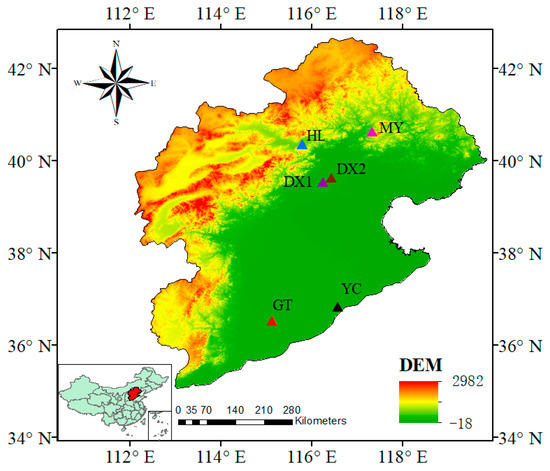
Figure 1.
Distribution of the six flux tower sites in the study area and the topographic characteristics of HRB. Daxing1 (DX1), Daxing2 (DX2), Guantao (GT), Huailai (HL), Miyun (MY) and Yucheng (YC).
2.2. Data Collection
2.2.1. Eddy Covariance Data
In our study, the machine-learning algorithms were validated and assessed using ground-observation flux tower data with remote-sensing and reanalysis data. All LE measurements were done using the eddy covariance (EC) method, which is regarded as the only standard method for directly measuring the material and energy exchanges between the biosphere and atmosphere. The data, covering the period from 2002 to 2013, were obtained from 6 EC flux tower sites and provided by Lathuileflux, the National Tibetan Plateau Data Center (TPDC) [35,36,37,38,39,40] and Chinaflux. These flux towers are located in China (112–120° east longitude, 35–43° north latitude, Table 1) and cover two land-surface biomes: mixed forests (DX1) and cropland (DX2, GT, HL, MY, YC). These sites recorded values every half-hour. The half-hour surface fluxes were linearly aggregated into daily mean values. The data are invalid when the amount of missing data exceeds 20% of the responsible half-hourly measurements. We removed the zero values and invalid values in the study. For the unclosed energy problem, we corrected the LE value for the six flux towers by the method developed by Twine et al. [41].

Table 1.
Information of the Six Flux Tower Sites Used in This Study.
2.2.2. Remote Sensing and Reanalysis Data
In our study, the following five parameters were used as characteristic variables to assess the performance of the three machine-learning methods for estimating LE: NDVI, DSR, RH, Ta, and WS. The GLASS NDVI product was produced by Xiao et al. and based on Advanced Very High-Resolution Radiometer (AVHRR) data with a temporal resolution of 8 days and a spatial resolution of 0.05° [42]. Then daily NDVI data with a resolution of 0.05° were obtained through temporal interpolation [43,44].
The daily DSR, RH, Ta, and WS products were obtained from the China meteorological forcing dataset (CMFD) provided by the National Tibetan Plateau Data Center (TPDC) with a temporal resolution of three hours and a spatial resolution of 0.1° [45,46,47]. To obtain the daily meteorological data product with a spatial resolution of 0.05°, the three-hour data were linearly aggregated into daily mean values, and we used the spatial interpolation method proposed by Zhao et al. [44] to interpolate the CMFD dataset. Theoretically, the method uses the 4 pixels around each pixel to eliminate sharp changes between adjacent pixels to improve the accuracy of the data.
3. Methods
3.1. Gradient Boosting Regression
The gradient boosting model is a widely used algorithm proposed by Friedman for classification and regression problems [24], which is a model composed of an ensemble of decision trees or regression trees: gradient boost decision trees (GBDTs) for classification and gradient boost regression tree (GBRTs) for regression. The diagram of the GBRT algorithm is shown in Figure 2 [48].
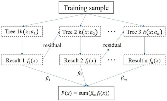
Figure 2.
Diagram of GBRT algorithm.
The approximation function for the GBRT can be expressed as follows,
where x represents the input variables and denotes the classifier of each decision tree. Each tree can be defined as , and denotes the weight for each tree.
In the GBRT model, the weak learner measures the errors in each node and uses the test function to split the node. All regression trees are interrelated, and the major advantage lies in that the tree in the GBRT is fitted based on the residual of the former tree. Therefore, the GBRT model can reduce the biases and is superior to other tree-based models for overfitting and cost calculation [29]. In addition, its advantage is associated with the ability to handle the uneven distribution of data attributes and has no restrictions on any assumptions of input data. Through the ensemble algorithm, the GBRT has better predictive capacity and stability than a single decision tree does.
3.2. Other Machine-Learning Methods
In our study, we choose two machine-learning algorithms (random forest, and extra tree regressor) to compare with the GBRT. These three algorithms are all based on regression and classification trees. However, they have different algorithm structures. They are widely used because they are relatively simple but powerful algorithms for dealing with classification and regression problems. Therefore, we estimate LE by these three methods in this study.
3.2.1. Random Forests
The random forest (RF) algorithm was proposed by Breiman (2001) [49]. It is a similar algorithm to the GBRT and uses an ensemble of a large set of decision trees. The difference between the RF and GBRT models is that the tree in the RF model is trained in parallel. To avoid the association of the different trees, RF creates different training subsets to increase the multiplicity of the trees. The RF algorithm is an extension of the bagging algorithm, and it uses either categorical or continuous predictor variables and either classification or continuous regression response variables. RF can reduce variance by ensemble different trees, sometimes at the cost of a slight increase in the bias. In the RF algorithm, some data may be used multiple times during training while others may never be used. Because the input data change slightly, the model achieves greater stability and improves prediction accuracy [50]. The other advantage of RF algorithms is that they can provide an evaluation of the importance of the different input parameters.
3.2.2. Extra Tree Regression
The extra tree regressor (ETR) algorithm is an averaging algorithm based on randomized decision trees, and it is similar to the RF algorithm and was proposed by Geurts [51]. The ETR and RF algorithms are combined techniques particularly designed for trees. In general, the ERT algorithm is used for classification and regression problems. The ETR ensemble method obtains its result by averaging the outcomes from many decision trees or regression trees. These trees are trained by dividing the origin dataset into subsets using simple rules derived from the parameter information. Compared with the RF, the ETR performs a further step by computing splits. As in the random forest method, a random train data subset of features is used, thresholds are randomly extracted for each feature, and the optimal of these randomly generated thresholds is selected as the splitting rule. This process usually results in an ETR model with a smaller variance than RF, but at the cost of a large bias.
3.3. Evaluation Methods
In this study, we use three general statistical indicators to compare and evaluate the accuracy of the machine-learning models for terrestrial LE estimation. The indicators include the coefficient of determination (R2, Equation (2)), root mean square error (RMSE, Equation (3)) and bias (Bias, Equation (4)). The mathematical equations of the indicators can be expressed as follows:
and are the observed and estimated values, respectively; and are the average of and ; and is the total number of the data.
3.4. Experimental Setup
For the training step, we used Python platform to build GBRT, RF and ETR models based on sklearn modules, and selected DSR, RH, Ta, WS and NDVI as input paraments and LE measured on the ground as output variables. The performance of three machine-learning models was evaluated through cross-validations, which entailed dividing the data into training and testing data and then training the model with the training dataset and verifying the accuracy of the model with the testing dataset. We conducted two experiments temporally and spatially: (1) the last year of all sites was tested, and (2) each site was removed from the training. Overall, the first cross-validation experiment assessed the uncertainty of the time series based on all flux sites, while the second cross-validation experiment was used to evaluate the uncertainty of the space series.
GBRT model parameters include the n_estimators, max_depth, min_samples_split learning_rate and loss. The main parameters of RF and ETR are n_estimators, max_features, max_depth, and min_samples_split. The performance of machine-learning algorithms are influenced by these parameters. The optimal parameter combination of the model can be obtained by constantly adjusting the parameters, which can improve the accuracy and efficiency of model estimation and also reduce the running time of the model. We found the optimal combination of parameters for each machine-learning method by the GridSearchCV module, which is a parameter-tuning method that attempts every possibility by iterating through all the parameter combinations to find the optimal parameter combination that can produce the best results. However, the main deficiency of this method is that it is time-consuming.
4. Results
4.1. Model Training and Validation from EC Observations
Three machine-learning algorithm LE estimates were generated using remote sensing and reanalysis data from all flux tower sites. Figure 3 shows the performance index results of the training and testing data in the temporal domain using the first cross-validation experiment in which the last year of all sites was tested and the other years were trained by the GBRT, RF and ETR models. The results showed that the GBRT model is slightly superior to the other models in the estimation of LE in the training period, having the highest values of R2 (0.81) and the lowest values of RMSE (22.4 W/m2). The RF and ETR models have lower R2 values (0.76 and 0.77, respectively) and higher RMSE values (26.2 W/m2 and 24.7 W/m2, respectively). For the testing data, the validation result showed that the R2 was very close among the three algorithms; however, the GBRT had a lower RMSE and bias than the RF and ETR.
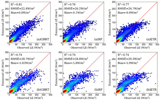
Figure 3.
The performance indices result of the training and testing data from the first cross-validation experiment (the last year of all sites were tested, and the others were trained) for the three machine-learning algorithms. (a): training results; (b): testing results.
Figure 4 shows the performance-index results of the testing data of each site in the temporal domain using the first cross-validation experiment. The results showed that the GBRT model estimates generally corresponded better to the ground-measured LE than the RF and ETR models did for most of the flux tower sites. At the six flux tower sites, the GBRT exhibited slightly better performance than the RF method, as indicated by the approximately 3.9% higher R2 value, 4.8% smaller RMSE, and 4.0% smaller Bias. Similarly, the GBRT results were 4.4% better for R2 than ETR, with a 4.6% smaller RMSE and 3.2% smaller Bias. In particular, the MY site had the highest R2, and the HL site had the lowest R2 at all sites.
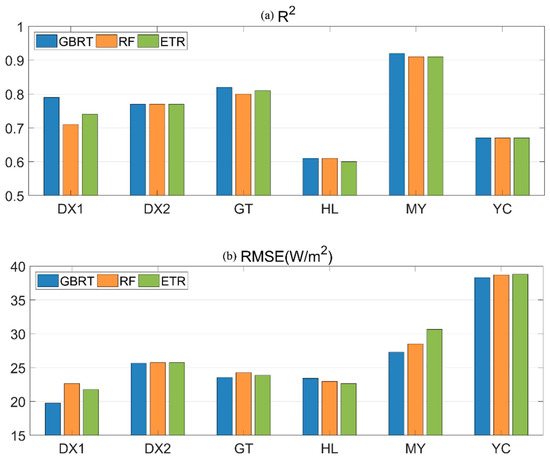
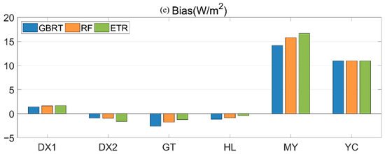
Figure 4.
The performance indices result of the testing data of the first cross-validation experiment of each site for the three machine-learning algorithms. (a): R2; (b): RMSE; (c): Bias.
We then validated the models in the spatial domain using the second cross-validation experiment in which one site was tested and the other sites were trained, with six repeats. Figure 5 shows the combined result of the testing data performance indices for all sites. The validation result shows that the GBRT had better performance than the RF and ETR algorithms, with a higher R2 value (0.69) and lower RMSE value (29.8 W/m2).
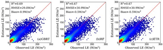
Figure 5.
The performance indices result of the testing data of the second cross-validation experiment (one site was tested, and the others site were trained) for the three algorithms. (a): GBRT; (b): RF; (c): ETR.
Figure 6 shows the performance index results of the testing data from the second cross-validation experiment of the GBRT, RF and ETR models at each site and shows that the estimated LE of the proposed model had better performance. Overall, the GBRT showed slightly better performance relative to the site measurements than did the RF and ETR at all flux tower sites and achieved an approximately 3.9% higher R2 and 1.9% smaller RMSE. For bias, the GBRT algorithms showed lower values at most sites.
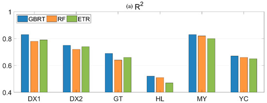
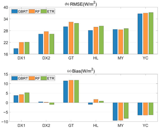
Figure 6.
The performance indices result of the testing data of the second cross-validation experiment (one site was tested, and the other sites were trained, circulating six times) of each site for three machine-learning algorithms. (a): R2; (b): RMSE; (c): Bias.
After two cross-validations, the performance of the three machine-learning methods proposed in this study was encouraging in the temporal and spatial domains. The model used ground-measurement data, remote-sensing, and reanalysis data, and included six sites distributed in the HRB. Therefore, the proposed machine-learning model has the ability to upscale site LE data to the regional scale across the HRB.
4.2. Implementation of Regional LE Estimation Using the GBRT
Our study is based on EC observations, CMFD meteorology and NDVI data to estimate daily LE using three machine-learning algorithms. To implement the regional LE estimation over the HRB, we retrained the GBRT, RF and ETR models based on data from the six sites. Figure 7 illustrates the performance index results of the retrained and probability density distributions of the predictive errors in the three machine-learning methods. The performance-index results of the three retrained models show that the GBRT was better than the RF and ETR models, with a higher R2 value (0.86) and lower RMSE value (18.1 W/m2). The probability density distributions of estimated errors of the estimated LE by the three machine-learning methods show that the predictive errors of all three machine-learning algorithms are close to zero. The GBRT method shows competitive results and has the best performance among the three machine-learning algorithms, while the ETR method had the worst performance over the HRB.
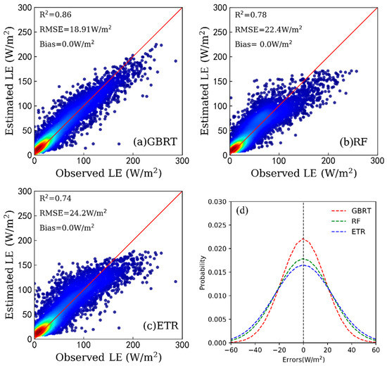
Figure 7.
The performance indices result of retrained and probability density distributions of the predictive errors in three machine-learning algorithms. (a): R2; (b): RMSE; (c): Bias; (d): probability density distributions of the predictive errors
Terrestrial LE is estimated by the retrained GBRT, RF and ETR models. For each site, we selected a year with complete observation data and plotted the eight-day average of ground measured LE and the corresponding LE estimation by three machine-learning methods, and the corresponding MODIS LE (MOD16A2, with a temporal resolution of 8 days). Figure 8 illustrates the eight-day terrestrial LE average of the ground-measured, estimated values by the three machine-learning algorithms and MODIS LE for the six sites. The estimated LE value showed great consistency with the ground-measured LE value for each site, and features that corresponded to the measured LE seasonality for different sites. On the contrary, compared with the ground-measured LE, the MODIS LE values are lower for six sites, and trends of MODIS LE and ground-measured LE varied significantly at the DX2 and HL sites.
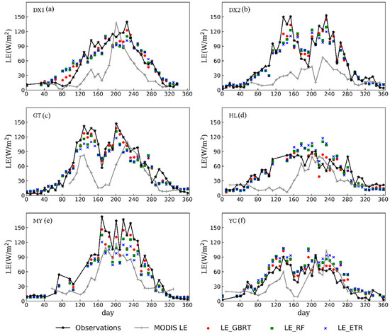
Figure 8.
Examples of the eight-day terrestrial LE average as measured and estimated using different machine-learning algorithms for the different sites. (a): DX1; (b): DX2;(c): GT; (d): HL; (e): MY; (f): YC.
However, model performance also varied with the site. Three algorithms all exhibited overestimation for DX1 from January to April and moderate underestimation from May to August, with the GT and MY sites showing large underestimations from June to August and the DX2 site showing an overestimation during the same period. In addition, the HL site showed an overestimation for summer and underestimation for winter, while the YC site showed an overestimation over the whole year. As shown in Figure 8, the GBRT method produced the closest LE estimation to the ground-observed values compared with the RF and ETR for the six flux-tower sites. Therefore, the GBRT method could be applied to estimate regional terrestrial LE over the HRB for 2016–2018.
4.3. Mapping of Terrestrial LE in the Haihe River Basin Based on the GBRT
Figure 9 shows the maps of average annual terrestrial LE from 2016 to 2018 based on the GBRT algorithms over the HRB with a resolution of 0.05°. The estimated differences in annual terrestrial LE were mainly distributed in the range of 30 to 70 W/m2 over the study area. The results show that the GBRT methods yielded lower LE estimates over the western portion in the center latitudes and estimated higher LE values in the eastern portions of the HRB. In addition, there is also a higher LE value in the southern HRB. The highest LE estimates occurred in the lowest latitude over the area, and the mean annual LE was approximately 66 W/m2.
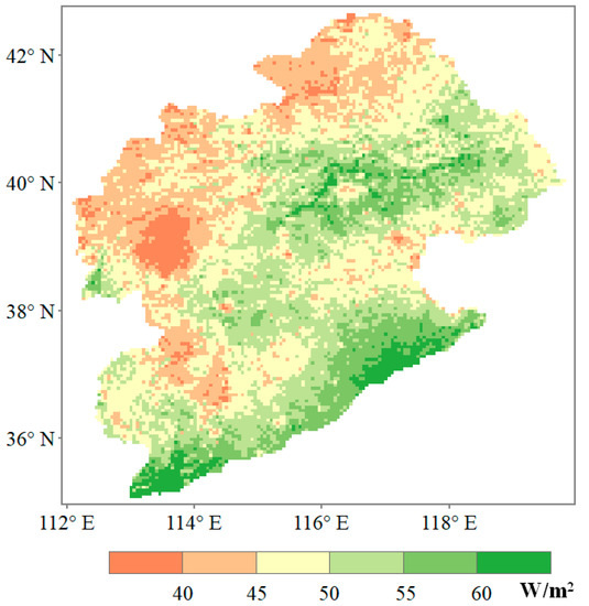
Figure 9.
Maps of average annual terrestrial LE in the period from 2016 to 2018 by using GBRT algorithms over HRB with a resolution of 0.05°.
Figure 10 shows the multiyear (2016–2018) mean seasonality for the GBRT model estimates. Large spatial variability and strong seasonality in the LE were observed. In spring (March–May), the estimated terrestrial LE was mainly distributed in the range of 40 to 60 W/m2. The LE in the southern area was higher than that in the northern part of the whole area; in addition, the LE value in the central part of the region was higher. In summer (June–August), the estimated terrestrial LE was mainly distributed in the range of 60 to 130 W/m2, and high LE values were observed in the 40° north latitude area of the HRB. The LE was considerably higher in summer than in other seasons. However, compared with other seasons, LE in summer was lower on the plain than in other areas. In fall (September–November), the estimated terrestrial LE was mainly distributed in the range of 20 to 60 W/m2. The plain in the southeast of the basin had a higher LE than the mountain area of the northwest. In winter (December–February), the terrestrial LE was estimated mainly below 20 W/m2 over the whole area. The LE magnitude was obviously lower than in the other seasons.
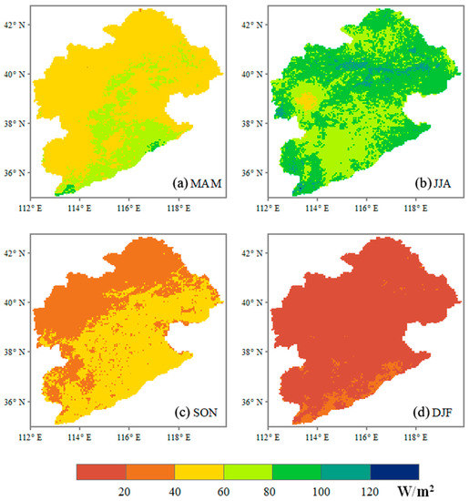
Figure 10.
Maps of mean seasonality terrestrial LE from 2016 to 2018 using GBRT algorithms over HRB with a resolution of 0.05°. (a): spring; (b): summer; (c): fall; (d): winter.
5. Discussion
5.1. Performance of the GBRT
The cross-validation results indicated that the test indicators of each site were different. We attributed the reasons for uncertainty in the validation process to different factors, such as the difference in geographical location and time period covered for each site. Some studies showed that that different elevations led to different LE values in the HRB [52]. The HL site is located at the junction of mountains and plains where the elevation is higher than at the other sites, which may explain the poor accuracy of the HL site in the cross-validation process. In addition, the dataset in our study covered different time periods at every site, and the time scale mismatch among the different sites may have resulted the lower performance of some sites during the validation process [5,33].
Figure 8 indicates that there is a slight difference between the ground observations and LE estimates by the three machine-learning methods. Errors were mainly caused by the biases of the EC observations and remote-sensing and reanalysis data as well as the mismatched spatial scales between datasets from different sources [53,54]. First, the prediction performances of the machine-learning algorithms were greatly affected by the quality of the EC observation data. The EC method is regarded as the only standard method for directly measuring the material and energy exchange between the biosphere and atmosphere although the EC observation method has the problem of energy imbalance [55]. The LE observations can be corrected by the formula [41] although they still had an error of approximately 5–20% [56], which would have reduced the accuracy of LE estimation by the machine-learning algorithms [57]. Second, several studies proved the uncertainties in reanalysis data and NDVI datasets. The reanalysis data and satellite-based vegetation parameter products were found to have had large errors during verification with ground observation data. [58]. The uncertainty of the LE estimates inherited the errors in the input data [59]. Third, mismatched spatial scales between different data sources also had an important influence on LE estimates [5]. The footprint of the flux tower site is approximately several hundred meters, which is smaller than the gridded data, including the CMFD and NDVI products.
The GBRT has been widely used because of its advantages [25,26,29,60]. In our study, we estimated the daily LE based on the six EC flux tower sites and corresponding meteorological data and NDVI data using different machine-learning methods. Although the terrestrial LE can be well predicted using the GBRT, RF, and ETR methods, the prediction performance for different algorithms was not the same. The GBRT had a better estimation result than the RF and ETR, and there were three reasons for this result. First, the GBRT algorithm had better stability and prediction accuracy in LE estimates [27]. Fan et al. compared four tree-based models and proved that the GBRT had better performance than the RF. Second, the GBRT is more suitable for small datasets [48]. In our study, the sample data used were limited, which was problematic because the RF and ETR require more sample data. Third, machine-learning presented an overfitting problem, which means that the model was too accurate to predict the existing data, but could not reliably predict the future data. However, the GBRT algorithm can avoid overfitting to some extent [61].
In our study, compared to the other two machine-learning algorithms, the GBRT had better performance, as well as certain limitations. First, the machine-learning algorithms had strong uncertainties, especially in adjustable parameters [58]. Uncertainty can be caused by erroneous input data, which leads to more errors. Second, all machine-learning algorithms had good local performance, but poor generalizability [58]. In addition, all of them were relatively unpredictable. In the future, we can combine machine-learning algorithms with other models to improve terrestrial LE estimations and reduce their uncertainties.
5.2. Comparison Between Different LE products
Figure 11 shows the spatial differences in annual terrestrial LE between the GLASS LE product and the LE product estimated using GBRT algorithms from 2016 to 2018. As shown in Figure 11, compared to the GLASS LE product, the proposed algorithms yielded a lower LE in most southern portions of the HRB but a higher LE in the northern HRB. The difference between the two products was small and less than or equal to 20 W/m2 in most areas. This finding may have been caused by the different structures of the two algorithms. GLASS LE is produced based on a five-process-based algorithms [62,63,64], which can be easily affected by various parameters, and our LE estimates were based on the GBRT method.
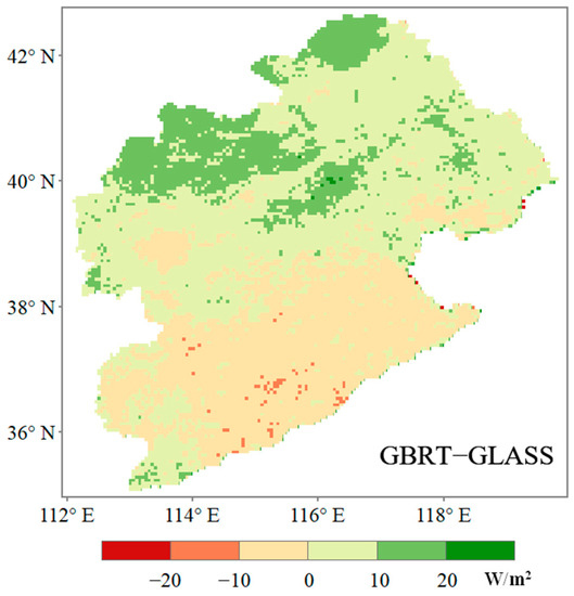
Figure 11.
Spatial differences in the average annual terrestrial LE (2016–2018) between GLASS LE product and LE product estimated using GBRT algorithms.
Figure 12 shows the spatial differences in the average annual terrestrial LE between the MODIS LE product and LE product estimated using GBRT algorithms over the HRB from 2016 to 2018. Relative to the MODIS LE product, the GBRT result showed lower LE in the north and southwest of the study area, but a higher LE in the plain area and in northwest area of the HRB. These differences may have been caused by the uncertainty of the quality and precision of EC observations, and the structure of the different machine-learning methods. In addition, the MODIS LE product presented certain errors [2,65], and did not provide value in areas that had no vegetation cover. Therefore, the simulation value of the machine-learning LE is slightly different from the value of the MODIS LE product over the study area, but the difference was less than 25 W/m2 in most areas.
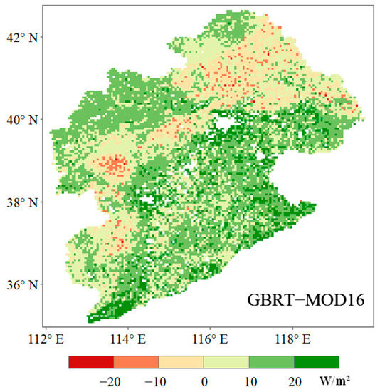
Figure 12.
Spatial differences in the average annual terrestrial LE (2016–2018) between MODIS LE product and LE product estimated using GBRT algorithms.
When compared with the GLASS LE and MODIS LE products, the LE estimated by the GBRT method had a relatively small gap, which showed that the proposed method was rational and feasible for estimating the LE over the HRB.
5.3. Implication of Terrestrial LE to Water Resources Management Over the Haihe River Basin
Water shortages have become a serious problem in the HRB [32,66,67,68]. Frequent droughts and increasingly serious shortages of water have hindered economic development and led to severe environmental problems [66]. Precipitation and LE are two indicators that play a leading role in drought hydrological systems. To date, most hydrologic studies have tended to focus on water supply, such as precipitation, but have largely ignored the loss of water through LE [67]. Terrestrial LE typically consumes approximately 60–90% of precipitation. Accurately measuring LE and its spatial and temporal variations, as an indicator of land water loss, is helpful for monitoring changes in vegetation and ecosystems and provides basic information for the study of hydrological system changes.
As a drought indicator, LE can capture the magnitude, intensity, and timing of drought for water resource management [68]. Quantitative assessments of terrestrial LE could facilitate the effective use of water resources in the HRB. In this study, we estimated the terrestrial LE over the HRB based on flux-tower observations, CMFD meteorological datasets and vegetation index data products using the GBRT, thereby proving that the GBRT algorithm has good predictive ability. Therefore, the proposed method of estimating terrestrial LE can provide a reference for the management and application of water resources in the HRB [69]. Estimating the LE in the HRB can significantly contribute to improving the environment and the proper use of water resources.
6. Conclusions
We applied three-machine-learning algorithms to estimate terrestrial LE based on flux tower observations, meteorological data from the China meteorological forcing dataset and the GLASS NDVI product over the HRB. Meteorological data and the GLASS NDVI were used as the input data, and LE observations were used as the output data to build the three models. We trained and validated three machine-learning algorithms at six EC flux tower sites and compared their prediction performance. The results showed that the GBRT algorithm achieved the best estimated accuracy with the highest R2 and the lowest Bias and RMSE during training and validation. A comparison with the GLASS LE and the MODIS LE products showed that the difference with the terrestrial LE by the GBRT algorithm was less than 20 W/m2 in most areas.
Overall, the GBRT method shows the best predictive ability among the three proposed methods based on the data of six flux sites and their corresponding meteorological data and NDVI data. Therefore, it can be concluded that the GBRT method is reasonable and reliable for estimating the terrestrial LE over the HRB.
Author Contributions
Conceptualization, Y.Z. and Y.Y.; resources, Z.X.; data curation, K.S., X.G. and J.Y.; validation, S.X. and J.W.; writing—original draft preparation, L.W.; All authors have read and agreed to the published version of the manuscript.
Funding
This work was supported by the Beijing–Tianjin–Hebei Collaborative Innovation Promotion Project, China (Z201100006720001), the Innovative Approaches Special Project of the Ministry of Science and Technology of China under Grant (2020IM020300), the National Natural Science Foundation of China under Grant 41671331, the National Key Research and Development Program of China under Grant 2016YFA0600103 and the Capital Normal University Multidisciplinary Studies Project, China (00719530012012, 00719530012010).
Institutional Review Board Statement
Not applicable.
Informed Consent Statement
Not applicable.
Data Availability Statement
3rd Party Data.
Acknowledgments
This work used eddy covariance data were obtained from the National Tibetan Plateau Data Center (TPDC) (https://data.tpdc.ac.cn/zh-hans/ (accessed on 31 January 2021)), the ChinaFLUX (http://www.chinaflux.org/ (accessed on 31 January 2021)), and the FLUXNET community (https://fluxnet.org/data/la-thuile-dataset/ (accessed on 31 January 2021)). The China meteorological forcing dataset (CMFD) were obtained from the TPDC (http://data.tpdc.ac.cn/en/ (accessed on 31 January 2021)). GLASS LE products provided by Beijing Normal University, China were obtained from online (http://glass-product.bnu.edu.cn/ (accessed on 31 January 2021)). MODIS LE products provided by NASA were obtained online (https://earthdata.nasa.gov/ (accessed on 31 January 2021)).
Conflicts of Interest
The authors declare no conflict of interest.
References
- Liang, S.; Wang, K.; Zhang, X.; Wild, M. Review on Estimation of Land Surface Radiation and Energy Budgets from Ground Measurement, Remote Sensing and Model Simulations. IEEE J. Sel. Top. Appl. Earth Obs. Remote Sens. 2010, 3, 225–240. [Google Scholar] [CrossRef]
- Mu, Q.; Zhao, M.; Running, S.W. Improvements to a MODIS global terrestrial evapotranspiration algorithm. Remote Sens. Environ. 2011, 115, 1781–1800. [Google Scholar] [CrossRef]
- Shukla, J.; Mintz, Y. Influence of Land-Surface Evapotranspiration on the Earth’s Climate. Science 1982, 215, 1498–1501. [Google Scholar] [CrossRef]
- Ortúñez, E.; De La Fuente, V. Typification of three taxa of the genusFestucaL. (Poaceae). Bot. J. Linn. Soc. 2008, 158, 342–343. [Google Scholar] [CrossRef]
- Yan, N.; Tian, F.; Wu, B.; Zhu, W.; Yu, M. Spatiotemporal Analysis of Actual Evapotranspiration and Its Causes in the Hai Basin. Remote Sens. 2018, 10, 332. [Google Scholar] [CrossRef]
- Trenberth, K.E.; Fasullo, J.T.; Kiehl, J. Earth’s Global Energy Budget. Bull. Am. Meteorol. Soc. 2009, 90, 311–324. [Google Scholar] [CrossRef]
- Jia, Z.; Liu, S.; Xu, Z.; Chen, Y.; Zhu, M. Validation of remotely sensed evapotranspiration over the Hai River Basin, China. J. Geophys. Res. Atmos. 2012, 117. [Google Scholar] [CrossRef]
- Li, Z.L.; Tang, R.; Wan, Z.; Bi, Y.; Zhou, C.; Tang, B.; Yan, G.; Zhang, X. A Review of Current Methodologies for Regional Evapotranspiration Estimation from Remotely Sensed Data. Sensors 2009, 9, 3801–3853. [Google Scholar] [CrossRef]
- Yao, Y.; Liang, S.; Li, X.; Zhang, Y.; Chen, J.; Jia, K.; Zhang, X.; Fisher, J.B.; Wang, X.; Zhang, L.; et al. Estimation of high-resolution terrestrial evapotranspiration from Landsat data using a simple Taylor skill fusion method. J. Hydrol. 2017, 553, 508–526. [Google Scholar] [CrossRef]
- Wu, B.; Yan, N.; Xiong, J.; Bastiaanssen, W.G.M.; Zhu, W.; Stein, A. Validation of ETWatch using field measurements at diverse landscapes: A case study in Hai Basin of China. J. Hydrol. 2012, 436–437, 67–80. [Google Scholar] [CrossRef]
- Wang, K.; Dickinson, R.E. A review of global terrestrial evapotranspiration: Observation, modeling, climatology, and climatic variability. Rev. Geophys. 2012, 50. [Google Scholar] [CrossRef]
- Xiong, J.; Wu, B.; Zhou, Y.; Li, J. Estimating Evapotranspiration using Remote Sensing in the Haihe Basin. In Proceedings of the 2006 IEEE International Symposium on Geoscience and Remote Sensing, Denver, CO, USA, 31 July–4 August 2006; pp. 1044–1047. [Google Scholar] [CrossRef]
- Ke, Y.; Im, J.; Park, S.; Gong, H. Downscaling of MODIS One Kilometer Evapotranspiration Using Landsat-8 Data and Machine Learning Approaches. Remote Sens. 2016, 8, 215. [Google Scholar] [CrossRef]
- Carter, C.; Liang, S. Evaluation of ten machine learning methods for estimating terrestrial evapotranspiration from remote sensing. Int. J. Appl. Earth Obs. Geoinf. 2019, 78, 86–92. [Google Scholar] [CrossRef]
- Glenn, E.P.; Nagler, P.L.; Huete, A.R. Vegetation Index Methods for Estimating Evapotranspiration by Remote Sensing. Surv. Geophys. 2010, 31, 531–555. [Google Scholar] [CrossRef]
- Verstraeten, W.W.; Veroustraete, F.; Feyen, J. Assessment of Evapotranspiration and Soil Moisture Content across Different Scales of Observation. Sensors 2008, 8, 70–117. [Google Scholar] [CrossRef]
- Liu, S.M.; Xu, Z.W.; Zhu, Z.L.; Jia, Z.Z.; Zhu, M.J. Measurements of evapotranspiration from eddy-covariance systems and large aperture scintillometers in the Hai River Basin, China. J. Hydrol. 2013, 487, 24–38. [Google Scholar] [CrossRef]
- Ruhoff, A.L.; Paz, A.R.; Aragao, L.E.O.C.; Mu, Q.; Malhi, Y.; Collischonn, W.; Rocha, H.R.; Running, S.W. Assessment of the MODIS global evapotranspiration algorithm using eddy covariance measurements and hydrological modelling in the Rio Grande basin. Hydrol. Sci. J. 2013, 58, 1658–1676. [Google Scholar] [CrossRef]
- Hu, G.; Jia, L. Monitoring of Evapotranspiration in a Semi-Arid Inland River Basin by Combining Microwave and Optical Remote Sensing Observations. Remote Sens. 2015, 7, 3056–3087. [Google Scholar] [CrossRef]
- Jin, Y.; Randerson, J.T.; Goulden, M.L. Continental-scale net radiation and evapotranspiration estimated using MODIS satellite observations. Remote Sens. Environ. 2011, 115, 2302–2319. [Google Scholar] [CrossRef]
- Dou, X.; Yang, Y. Evapotranspiration estimation using four different machine learning approaches in different terrestrial ecosystems. Comput. Electron. Agric. 2018, 148, 95–106. [Google Scholar] [CrossRef]
- Jung, M.; Reichstein, M.; Bondeau, A. Towards global empirical upscaling of FLUXNET eddy covariance observations: Validation of a model tree ensemble approach using a biosphere model. Biogeosciences 2009, 6, 2001–2013. [Google Scholar] [CrossRef]
- Yang, F.; White, M.A.; Michaelis, A.R.; Ichii, K.; Hashimoto, H.; Votava, P.; Zhu, A.; Nemani, R.R. Prediction of Continental-Scale Evapotranspiration by Combining MODIS and AmeriFlux Data Through Support Vector Machine. IEEE Trans. Geosci. Remote Sens. 2006, 44, 3452–3461. [Google Scholar] [CrossRef]
- Friedman, J.H. Stochastic gradient boosting. Comput. Stat. Data Anal. 2002, 38, 367–378. [Google Scholar] [CrossRef]
- Ma, H.; Yang, X.; Mao, J.; Zheng, H. The Energy Efficiency Prediction Method Based on Gradient Boosting Regression Tree. In Proceedings of the 2018 2nd IEEE Conference on Energy Internet and Energy System Integration (EI2), Beijing, China, 20–22 October 2018; pp. 1–9. [Google Scholar] [CrossRef]
- Wei, L.; Yuan, Z.; Zhong, Y.; Yang, L.; Hu, X.; Zhang, Y. An Improved Gradient Boosting Regression Tree Estimation Model for Soil Heavy Metal (Arsenic) Pollution Monitoring Using Hyperspectral Remote Sensing. Appl. Sci. 2019, 9, 1943. [Google Scholar] [CrossRef]
- Wei, Z.; Meng, Y.; Zhang, W.; Peng, J.; Meng, L. Downscaling SMAP soil moisture estimation with gradient boosting decision tree regression over the Tibetan Plateau. Remote Sens. Environ. 2019, 225, 30–44. [Google Scholar] [CrossRef]
- Yang, L.; Zhang, X.; Liang, S.; Yao, Y.; Jia, K.; Jia, A. Estimating Surface Downward Shortwave Radiation over China Based on the Gradient Boosting Decision Tree Method. Remote Sens. 2018, 10, 185. [Google Scholar] [CrossRef]
- Fan, J.; Yue, W.; Wu, L.; Zhang, F.; Cai, H.; Wang, X.; Lu, X.; Xiang, Y. Evaluation of SVM, ELM and four tree-based ensemble models for predicting daily reference evapotranspiration using limited meteorological data in different climates of China. Agric. For. Meteorol. 2018, 263, 225–241. [Google Scholar] [CrossRef]
- Feng, Y.; Cui, N.; Gong, D.; Zhang, Q.; Zhao, L. Evaluation of random forests and generalized regression neural networks for daily reference evapotranspiration modelling. Agric. Water Manag. 2017, 193, 163–173. [Google Scholar] [CrossRef]
- Shang, K.; Yao, Y.; Li, Y.; Yang, J.; Jia, K.; Zhang, X.; Chen, X.; Bei, X.; Guo, X. Fusion of Five Satellite-Derived Products Using Extremely Randomized Trees to Estimate Terrestrial Latent Heat Flux over Europe. Remote Sens. 2020, 12, 687. [Google Scholar] [CrossRef]
- Guo, Y.; Shen, Y. Quantifying water and energy budgets and the impacts of climatic and human factors in the Haihe River Basin, China: 2. Trends and implications to water resources. J. Hydrol. 2015, 527, 251–261. [Google Scholar] [CrossRef]
- Li, X.; Gemmer, M.; Zhai, J.; Liu, X.; Su, B.; Wang, Y. Spatio-temporal variation of actual evapotranspiration in the Haihe River Basin of the past 50 years. Quat. Int. 2013, 304, 133–141. [Google Scholar] [CrossRef]
- Yang, H.; Yang, D.; Lei, Z.; Sun, F.; Cong, Z. Variability of complementary relationship and its mechanism on different time scales. Sci. China Ser. E 2009, 52, 1059–1067. [Google Scholar] [CrossRef]
- Liu, S.; Xu, Z. Multi-scale surface flux and meteorological elements observation dataset in the Hai River Basin (Guantao site-eddy covariance system) (2008–2010). Natl. Tibet. Plateau Data Cent. 2016. [Google Scholar] [CrossRef]
- Liu, S.; Xu, Z. Multi-scale surface flux and meteorological elements observation dataset in the Hai River Basin (Miyun site-eddy covariance system) (2008–2010). Natl. Tibet. Plateau Data Cent. 2016. [Google Scholar] [CrossRef]
- Liu, S.; Xu, Z. Multi-scale surface flux and meteorological elements observation dataset in the Hai River Basin (Daxing site—eddy covariance system) (2008–2010). Natl. Tibet. Plateau Data Cent. 2016. [Google Scholar] [CrossRef]
- Xu, Z.; Liu, S. Multi-scale surface flux and meteorological elements observation dataset in the Hai River Basin (Huailai station-eddy covariance system-10m tower, 2013). Natl. Tibet. Plateau Data Cent. 2016. [Google Scholar] [CrossRef]
- Liu, S.; Xu, Z. Multi-scale surface flux and meteorological elements observation dataset in the Hai River Basin (Huailai station-eddy covariance system-10m tower, 2014). Natl. Tibet. Plateau Data Cent. 2016. [Google Scholar] [CrossRef]
- Guo, A.; Liu, S.; Zhu, Z.; Xu, Z.; Xiao, Q.; Ju, Q.; Zhang, Y.; Yang, X. Impact of Lake/Reservoir Expansion and Shrinkage on Energy and Water Vapor Fluxes in the Surrounding Area. J. Geophys. Res. Atmos. 2020, 125. [Google Scholar] [CrossRef]
- Twine, T.E.; Kustas, W.P.; Norman, J.M.; Cook, D.R.; Houser, P.R.; Meyers, T.P.; Prueger, J.H.; Starks, P.J.; Wesely, M.L. Correcting eddy-covariance flux underestimates over a grassland. Agric. For. Meteorol. 2000, 103, 279–300. [Google Scholar] [CrossRef]
- Xiao, Z.; Liang, S.; Tian, X.; Jia, K.; Yao, Y.; Jiang, B. Reconstruction of Long-Term Temporally Continuous NDVI and Surface Reflectance From AVHRR Data. IEEE J. Sel. Top. Appl. Earth Obs. Remote Sens. 2017, 10, 5551–5568. [Google Scholar] [CrossRef]
- Huete, A.; Didan, K.; Miura, T.; Rodriguez, E.P.; Gao, X.; Ferreira, L.G. Overview of the radiometric and biophysical performance of the MODIS vegetation indices. Remote Sens. Environ. 2002, 83, 195–213. [Google Scholar] [CrossRef]
- Zhao, M.; Heinsch, F.A.; Nemani, R.R.; Running, S.W. Improvements of the MODIS terrestrial gross and net primary production global data set. Remote Sens. Environ. 2005, 95, 164–176. [Google Scholar] [CrossRef]
- Yang, K.; He, J. China meteorological forcing dataset (1979–2018). National Tibetan Plateau Data Center, 2019. [Google Scholar]
- He, J.; Yang, K.; Tang, W.; Lu, H.; Qin, J.; Chen, Y.; Li, X. The first high-resolution meteorological forcing dataset for land process studies over China. Sci. Data 2020, 7, 25. [Google Scholar] [CrossRef]
- Yang, K.; He, J.; Tang, W.; Qin, J.; Cheng, C.C.K. On downward shortwave and longwave radiations over high altitude regions: Observation and modeling in the Tibetan Plateau. Agric. For. Meteorol. 2010, 150, 38–46. [Google Scholar] [CrossRef]
- Liang, W.; Luo, S.; Zhao, G.; Wu, H. Predicting Hard Rock Pillar Stability Using GBDT, XGBoost, and LightGBM Algorithms. Mathematics 2020, 8, 765. [Google Scholar] [CrossRef]
- Breiman, L. Random Forests. Mach. Learn. 2001, 45, 5–32. [Google Scholar] [CrossRef]
- Rodriguez-Galiano, V.; Sanchez-Castillo, M.; Chica-Olmo, M.; Chica-Rivas, M. Machine learning predictive models for mineral prospectivity: An evaluation of neural networks, random forest, regression trees and support vector machines. Ore Geol. Rev. 2015, 71, 804–818. [Google Scholar] [CrossRef]
- Geurts, P.; Ernst, D.; Wehenkel, L. Extremely randomized trees. Mach. Learn. 2006, 63, 3–42. [Google Scholar] [CrossRef]
- Wu, X.; Meng, D. Analysis of temporal and spatial characteristics about surface actual Evapotranspiration in Haihe river basin based on MODIS. In Proceedings of the 2016 4th International Workshop on Earth Observation and Remote Sensing Applications (EORSA) 2016, Guangzhou, China, 4–6 July 2016; pp. 456–460. [Google Scholar] [CrossRef]
- Sagi, O.; Rokach, L. Ensemble learning: A survey. Wires Data Min. Knowl. Discov. 2018, 8, e1249. [Google Scholar] [CrossRef]
- Aytug, H.; Bhattacharyya, S.; Koehler, G.J.; Snowdon, J.L. A review of machine learning in scheduling. IEEE Trans. Eng. Manag. 1994, 41, 165–171. [Google Scholar] [CrossRef]
- Foken, T. The energy balance closure problem: An overview. Ecol. Appl. 2008, 18, 1351–1367. [Google Scholar] [CrossRef] [PubMed]
- Yao, Y.; Liang, S.; Yu, J.; Chen, J.; Liu, S.; Lin, Y.; Fisher, J.B.; Mcvicar, T.R.; Cheng, J.; Jia, K.; et al. A simple temperature domain two-source model for estimating agricultural field surface energy fluxes from Landsat images. J. Geophys. Res. Atmos. 2017, 122, 5211–5236. [Google Scholar] [CrossRef]
- Yao, Y.; Liang, S.; Li, X.; Chen, J.; Liu, S.; Jia, K.; Zhang, X.; Xiao, Z.; Fisher, J.B.; Mu, Q.; et al. Improving global terrestrial evapotranspiration estimation using support vector machine by integrating three process-based algorithms. Agric. For. Meteorol. 2017, 242, 55–74. [Google Scholar] [CrossRef]
- Zhao, M.; Running, S.W.; Nemani, R.R. Sensitivity of Moderate Resolution Imaging Spectroradiometer (MODIS) terrestrial primary production to the accuracy of meteorological reanalyses. J. Geophys. Res. 2006, 111, G01002. [Google Scholar] [CrossRef]
- Mu, Q.; Heinsch, F.A.; Zhao, M.; Running, S.W. Development of a global evapotranspiration algorithm based on MODIS and global meteorology data. Remote Sens. Environ. 2007, 111, 519–536. [Google Scholar] [CrossRef]
- Ponraj, A.S.; Vigneswaran, T. Daily evapotranspiration prediction using gradient boost regression model for irrigation planning. J. Supercomput. 2020, 76, 5732–5744. [Google Scholar] [CrossRef]
- Kotsiantis, S.B. Decision trees: A recent overview. Artif. Intell. Rev. 2013, 39, 261–283. [Google Scholar] [CrossRef]
- Yao, Y.; Liang, S.; Li, X.; Hong, Y.; Fisher, J.B.; Zhang, N.; Chen, J.; Cheng, J.; Zhao, S.; Zhang, X.; et al. Bayesian multimodel estimation of global terrestrial latent heat flux from eddy covariance, meteorological, and satellite observations. J. Geophys. Res. Atmos. 2014, 119, 4521–4545. [Google Scholar] [CrossRef]
- Yao, Y.; Liang, S.; Cheng, J.; Liu, S.; Fisher, J.B.; Zhang, X.; Jia, K.; Zhao, X.; Qin, Q.; Zhao, B.; et al. MODIS-driven estimation of terrestrial latent heat flux in China based on a modified Priestley–Taylor algorithm. Agric. For. Meteorol. 2013, 171–172, 187–202. [Google Scholar] [CrossRef]
- Yao, Y.; Liang, S.; Li, X.; Chen, J.; Wang, K.; Jia, K.; Cheng, J.; Jiang, B.; Fisher, J.B.; Mu, Q.; et al. A satellite-based hybrid algorithm to determine the Priestley-Taylor parameter for global terrestrial latent heat flux estimation across multiple biomes. Remote Sens. Environ. 2015, 165, 216–233. [Google Scholar] [CrossRef]
- Kim, H.W.; Hwang, K.; Mu, Q.; Lee, S.O.; Choi, M. Validation of MODIS 16 global terrestrial evapotranspiration products in various climates and land cover types in Asia. Ksce J. Civ. Eng. 2012, 16, 229–238. [Google Scholar] [CrossRef]
- Jiaqi, C.; Jun, X. Facing the challenge: Barriers to sustainable water resources development in China. Hydrol. Sci. J. 1999, 44, 507–516. [Google Scholar] [CrossRef]
- Fisher, J.B.; Melton, F.; Middleton, E.; Hain, C.; Anderson, M.; Allen, R.; McCabe, M.F.; Hook, S.; Baldocchi, D.; Townsend, P.A.; et al. The future of evapotranspiration: Global requirements for ecosystem functioning, carbon and climate feedbacks, agricultural management, and water resources. Water Resour. Res. 2017, 53, 2618–2626. [Google Scholar] [CrossRef]
- Cai, X. Water stress, water transfer and social equity in Northern China—Implications for policy reforms. J. Environ. Manag. 2008, 87, 14–25. [Google Scholar] [CrossRef] [PubMed]
- Berner, L.T.; Beck, P.S.A.; Loranty, M.M.; Alexander, H.D.; Mack, M.C.; Goetz, S.J. Cajander larch (Larix cajanderi) biomass distribution, fire regime and post-fire recovery in northeastern Siberia. Biogeosciences 2012, 9, 3943–3959. [Google Scholar] [CrossRef]
Publisher’s Note: MDPI stays neutral with regard to jurisdictional claims in published maps and institutional affiliations. |
© 2021 by the authors. Licensee MDPI, Basel, Switzerland. This article is an open access article distributed under the terms and conditions of the Creative Commons Attribution (CC BY) license (http://creativecommons.org/licenses/by/4.0/).