Abstract
Identifying precursor events that allow the timely forecasting of landslides, thereby enabling risk reduction, is inherently difficult. Here we present a novel, low cost, flow visualization technique using time-lapsed imagery (TLI) that allows real time analysis of slope movement. This approach is applied to the Rest and Be Thankful slope, Argyle, Scotland, where past debris flows have blocked the A83 or forced preemptive closure. TLI of the Rest and Be Thankful are taken from a fixed station, 28 mm lens, time lapse camera every 15 min. Imagery is filtered to counter the effects of misalignment from wind induced vibration of the camera, asymmetric lighting, and fog. Particle image velocimetry (PIV) algorithms are then run to produce slope movement velocity vectors. PIV generated vectors are automatically post-processed to separate vectors generated by slope movement from false positives generated by harsh environmental conditions. Results for images over a 20-day period indicated precursor slope movement initiated by a rainfall event, a period of quiescence for 10 days, followed by a large landslide failure during proceeding rainfall where over 3000 tons of sediment reached the road. Results suggest low cost, live streamed TLI and this novel PIV approach correctly detect and, importantly, report precursor slope movement, allowing early warning, effective management and landslide impact mitigation. Future applications of this technique will allow the development of an effective decision-making tool for asset management of the A83, reducing the risk to life of motorists. The technique can also be applied to other critical infrastructure sites, allowing hazard risk reduction.
1. Introduction
Slope failures pose a significant threat to human lives, infrastructure, and accessibility of assets. Climatic changes are altering the severity and variability of seasonal extremes and heightened storm intensity has been linked with higher numbers of recorded landsides [1,2]. Spatial and temporal variability in both forcing events such as rainfall delivery and ground saturation levels and in the complex responses of slope materials result in severe challenges to operational management decisions when assets or people are at risk. The initiation and subsequent development of landslides can be considerably removed from identifiable triggering events posing significant challenges to the identification of areas where slopes are undergoing the early stages of deformation and failure. Seismic monitoring systems have proven effective for the development of deep-seated failure processes or the live detection of events, but are limited in the identification and location of precursory movement, which do not produce the same strength of signal. High resolution terrestrial laser scanning [3] and Ground Based Synthetic Aperture Radar Interferometry [4,5] are capable of detailing failure processes, but such approaches rely on power supplies that are typically not suitable for the remote locations where landslides often happen because of their prohibitive cost.
Here we present a low-cost, accessible, portable and readily field deployable slope movement detection/monitoring system based on new analysis of standard optical time-lapse imagery. The proposed system is based on the principles of particle image velocimetry (PIV) where sequences of time-lapse images (TLI) from an off-the-shelf system comprising a Digital Single-Lens Reflex (DSLR), programmable intervalometer, running from solar rechargeable batteries streaming data via a 3G driven slope-wide WiFi network, are cross-correlated to obtain a set of velocity vectors that represents any movement in the slope [6]. The PIV analysis requires sufficient coverage and quality of the pre- and post-movement images to be achieved. This can be considered a challenge because the natural environment is often characterized by complex lighting, contrast patterns, and varied topography that leads to uneven pixel ground sampling—all typical in hazardous slope environments. Thus, the TLI are first pre-processed for contrast equalization, cloud detection, and image alignment before they are cross-correlated. Once the frame of velocity vectors is generated, it is post-processed by applying a set of de-noising filters. If a movement of the slope is detected, the system automatically generates an alarm and points out the area where the movement was observed. Here we detail the development of this processing workflow and apply it to an extensive (1 km wide) slope directly above the vital A83 arterial road connecting people and businesses between west and central Scotland. The method is used in order to detect and report any precursory slope movements and failure developments to stakeholders responsible for managing landslide risk on the network–in this instance, Transport Scotland.
Site and Setup
The A83 Rest and Be Thankful has been used as an exemplar of a chronic landslide risk hotspot, where precursory deformation had often been noted by stakeholders. The Rest and Be Thankful is a key tourist stop and principal trunk road into the west of Scotland, affected by a particularly high frequency of landslides.
The A83 bisects the lower part of the slope which rises approximately 530 m from the floor of Glen Croe (133 m.asl). Below the A83 the Old Military Road, a single carriageway that runs parallel to the main road along the valley floor is used as an alternate route if the A83 is landslide impacted, though this too has been disrupted by larger landslides. In 2020–21, as a result of debris flow activity the A83 was closed for approximately 120 days. It is estimated that the disruption caused by these events, on average, cost the authorities £90,000 daily [7]. The volumetric magnitude of debris flows source areas ranged from 1.28 m3 to 333 m3, whilst creep movements (which did not immediately lead to a debris-flow and are difficult to place volume estimates on) affected areas ranging from 7.34 m2 to 1584.62 m2.
The site is a glacially conditioned valley comprised predominantly of steep-sided rock slopes draped with glacial till and colluvium on the lower slopes and valley floor [8]. The bedrock consists of Neoproterozoic pelite, semipelite, and psammite, with an overlying layer of densely gullied till up to 3 m thick and interspersed with shallow scars, levees and debris cones. The slope has a concave bowl at the top, likely a cirque, (Figure 1) which appears to concentrate stream flow into the center of the slope, which Sparkes et al. [9] hypothesized could partly explain the predisposition of failures in this part of the slope. The site map of Glen Croe is shown in Figure 1a and its digital terrain model with the location of time-lapse camera is shown in Figure 1b.
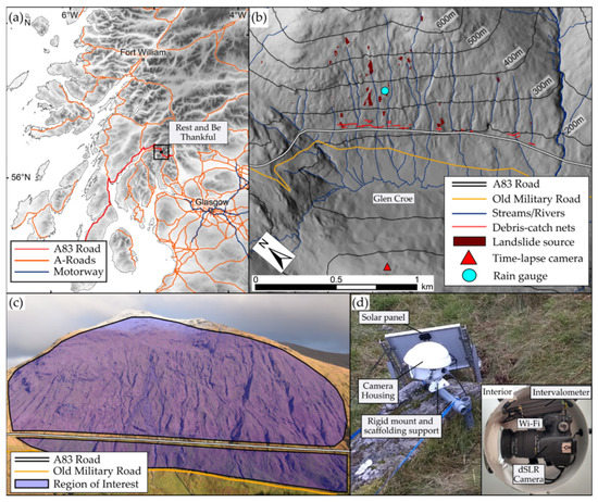
Figure 1.
(a) Site location map, (b) Site digital terrain model, (c) Time-lapse camera optical view, (d) Field setup of time-lapse camera and equipment.
A Nikon D810 DSLR with a 36-megapixel optical sensor and equipped with a fixed 28 mm lens is used to obtain imagery data at Rest and Be Thankful. The installation was placed at the opposite valley side of Glen Croe to the A83, approximately 1500 m from the Rest and Be Thankful slope. The camera faces straight on to the slope, i.e., does not have an oblique view. A custom programmable Cyclapse Digisnap Pro intevalometer is used to trigger photos every 15 min during daylight hours and a 50-watt solar panel is fitted to the unit to charge two Lithium Polymer (LiPo) batteries. Imagery was sent via WiFi to a nearby off-grid base-station where a 3G internet connection transmits the data for processing. For truly remote areas with no 3G/4G connectivity, the same setup can be used with alternative communication and processing methods. For scenarios where communication capabilities are limited, the detection algorithms can be implemented locally on site and the outcomes relevant to decisions can be sent via low power wide-area networks such as LoRa (Long Range). This architecture is especially advantageous to establish a network of nodes operating within a range of a few kilometers. The range constraint can be eliminated using satellite-based internet connection. However, the requirement of additional satellite receiver will add to the overall cost of the system. The field setup of time-lapse camera equipment for the experiments performed in this article is shown in Figure 1d.
2. Materials and Methods
2.1. PIV Image Analysis
PIV is an image-based velocity measurement technique used in fluid dynamics to measure the velocity field (direction and speed) of fluids. PIV is an indirect measurement technique where the fluid is first seeded with small particles called the tracers. The tracers are optimized to follow the motion of the fluid without disturbing its velocity field. This faithful motion of the tracers is quantified by Stoke’s number, which is directly proportional to the velocity of the fluid and inversely proportional to the diameter of the tracer particle [10]. Once the fluid is seeded, the tracers are illuminated with help of laser pulses (white light LEDs are used as a low-cost alternative) with known temporal frequency. During the illumination period, an optical sensor is used to take a snapshot of the fluid, thus obtaining the positions of the illuminated tracer particles. It is therefore vital that the laser pulses and the optical sensor’s shutter are perfectly synchronized. The images obtained by the optical sensor are divided into small regions called interrogation areas (IAs). The corresponding IAs from two images, for example: image A captured at the time t1 and image B captured at t2 are cross-correlated to obtain the displacement at t2 = t1 + Δt along the horizontal (x) and vertical (y) directions of the imaged tracers. Once the displacement has been determined, the x-component u and the y-component v of the velocity vector can be calculated if Δt is known. To calculate the z-component of the velocity vectors, a dual camera setup is required and the process is referred to as stereoscopic PIV, which is beyond the scope of this paper but could hold significant potential where the amount of progressive movement is of critical concern. This concept is illustrated in Figure 2 for one IA. The cross-correlation between two images is implemented as [11,12]:
where A and B are the corresponding areas of interrogation and m and n determines the shift of B in x and y direction, with respect to its identified position in A. The resulting matrix C holds a set of all possible in the image. The most probable displacement is then obtained as an intensity peak in C. Equation (1) can be solved in either the spatial domain (direct cross-correlation) or the frequency domain (discrete Fourier transform). Both these techniques and their derivates have been studied extensively in the literature [12,13,14,15].
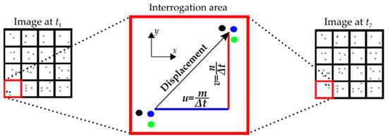
Figure 2.
Graphical illustration of PIV.
2.2. The PIVlab
PIVlab is an open-source graphical user interface created by William Thielicke [12,16] that implements PIV analysis of carefully controlled laboratory grayscale image sequences using different correlation functions (discrete Fourier transform and ensemble correlation), a batch of pre-processing image filters, and a number post-processing algorithms. Here we exploit and develop several inbuilt features of PIVlab to adapt it to the challenges of image sequences from a dynamic natural environment. The following inbuilt functionalities of PIVlab are embedded within all processes presented in this article (i) contrast limited adaptive histogram equalization (CLAHE); (ii) Intensity Capping; (iii) Multiple interrogation areas. These three features of PIVlab are reproduced here for the completion of this article with references to more detailed descriptions where applicable.
2.2.1. CLAHE
CLAHE was originally developed for the analysis of images in medical research applications [17]. Histogram equalization is a contrast optimization technique where the more frequent pixel intensities are spread across the whole spectrum of the image. For an n-bit image, this spectrum ranges from 0 to 2n−1. CLAHE is an advanced version of conventional histogram equalization in the sense that the image is first sectioned into several small windows (in PIVlab the window size can be adjusted in the image pre-processing settings). Histogram equalization is then performed independently on each of these windows. These equalized windows are then interpolated together, which removes the visible boundaries between two adjacent windows. This results in a flatter histogram than the application of a single histogram equalization applied across the full image.
2.2.2. Intensity Capping
A common source of bias and false detections in a frame generated by PIV arises due to the presence of pixels with a much higher than average greyscale intensity within the interrogation area. This source of error is more pronounced if PIV is used on images with inhomogeneous lighting. For landslide monitoring in naturally lit environments with variable cloud cover, this results in dynamic patterns of sunlight and shade across the slope. The presence of bright spots overwhelms the cross-correlation function, introducing bias in the output of PIV. However, this effect can be significantly reduced by upper bounding the intensities of all pixels in the greyscale image. This procedure is called intensity capping [18] and has been applied to all image analyses presented here.
2.2.3. Multiple Interrogation Areas
One of the most important parameters of PIV is the dimensions of the IA. A large IA captures the high-velocity motion of the tracer while a small IA is suitable for low velocity motion. The PIVlab allows the user to have multiple IAs of different sizes to capture both high and low-velocity components within the same sequence. This multiscale analysis increases the signal to noise ratio of the correlation significantly. All results in this study are obtained using three interrogation areas of the sizes 64 × 64, 32 × 32 and 16 × 16 pixels (for the Rest and Be Thankful example this equates to 10.24 m × 10.24 m, 5.12 m × 5.12 m, 2.56 m × 2.56 m, respectively). These areas encompass the range of slope movements (shallow surficial movements, deep-seated rotational slides, and channelized debris flows) historically detected on the slope [9]. In PIVlab the multiple interrogation areas can be set within the window of the graphical user interface.
PIVlab provides several pre- and post-processing filters, but the results obtained using outdoor TLI for landslide detection were unacceptable, with a large number of false-positives in every frame. Thus, in order to achieve sufficient feature tracking on image sequences of an uncontrolled slope environment, new filters and processing interventions have been added.
3. Progressing PIVlab for Landslide Monitoring Applications
Several limitations were observed in the application of PIVlab to landslide detection using field derived TLI sequences. False positives generated by uncontrolled environmental elements such as wind, cloud, and rain required unacceptable manual scrutiny and undermine efforts to allow automated wide-area deformation identification and tracking with minimal user intervention. Here we describe an improvement of PIVLab which aims to overcome the limitations which were initially observed in its application to landslide detection. The new features presented here have been added without compromising the structure of PIVlab graphical user interface and have been integrated so that they can be enabled or disabled within the original graphical user interface platform.
3.1. Amorphous & Multiple Regions of Interest
One of the major sources of noise in the velocimetry results obtained, studying the Rest and Be Thankful site used as our example, was the dynamics of the sky recorded in the background of the TLI. Since only one rectangular region of interest (ROI) could be selected in PIVlab, it was impossible to cover the full slope of Rest and be Thankful without including the background. Further, the full slope is split into two discrete sections by the A83 and the old military road. The inclusion of upper and lower segmented sections of the slope was impossible without including the roads, which generates significant noise in the analysis from moving vehicles. Therefore, a new feature was added where multiple amorphous user defined ROIs could be processed. This advance enabled the critical slope area to be included within two ROI polygons that exclude the main sources of noise.
3.2. Image Registration
PIV is ideally suited for laboratory tests using a fixed and stable camera system. Thus, image registration is not a mandatory prerequisite. However, the optical sensor used for landslide detection was exposed to the natural environment with particular difficulties related to the strong vibration caused by wind and the instability of the ground (soil movement, often linked to wetting/drying over variable time scales, daily to seasonal). These variations resulted in PIV producing velocity vectors throughout the defined ROIs in the opposite direction to the camera movement across successive frames (Figure 3a). These erroneous vectors, typically caused by wind induced vibration, required the development of a robust image registration algorithm to align the images prior to applying PIV on the TLI.
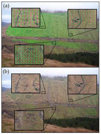
Figure 3.
Phase alignment of two images from the same fixed position, captured 15 min apart and no genuine slope movement was recorded between images. (a) Before phase alignment, (b) After phase alignment.
Phase correlation can be used to measure the linear phase component of a moving image in the frequency domain. This change in phase results from translations in horizontal x and vertical y directions of the same image to an altered position. Consider, for example, an M × N original image position A(i,j) has been shifted to a new position =. Evaluating the fast-Fourier transform (FFT) of A and one can obtain
where XA is the FFT of the fixed image A, and m and n are the directional shifts of in x and y directions, respectively when referenced to A. The next step involves taking the cross-correlation of the fast-Fourier transform of the two images defined by Equations (2) and (3), which results in:
where represents the complex conjugate of a function (.). The translation in horizontal and vertical directions of the shifted image can be established by taking the inverse discrete Fourier transform (iDFT) of (4), which results in a Dirac delta function centered at (−m, −n).
Equation (5), captures the successive translation caused by horizontal and vertical image shifts. The alignment of a shifted image can thus be obtained by translating it by the negative of m pixels in horizontal direction and n pixels in the vertical direction. This process and its impact on vector differences between the images is demonstrated in Figure 3; the velocity vectors generated by PIV here are the result of misalignment in images captured 15 min apart from a fixed position, exposed to wind vibrations (Figure 3a). Erroneous displacement vectors are largely eliminated using the phase correlation alignment (Figure 3b).
3.3. Live Monitoring with Dynamic Framerate
The current version of PIVlab was only capable of processing a preselected batch of images. In order to address this limitation for real-time monitoring applications, a real-time image processing workflow is required. The TLI obtained were uploaded to cloud services at 15-min intervals. These images were automatically read into a folder used by PIVlab, enabling the processing workflow to be continually updated with new images from the cloud. This additional feature allowed vector displacement monitoring from anywhere in near-real time and by multiple computers if required.
One of the limitations of PIVlab is the requirement of a static temporal frequency of the optical sensor. Conventionally, in laboratory environments, the framerate of an optical sensor is known a priori and it remains constant during the experiment. In a natural environment, the variable conditions mean that consecutive images may not always be useable (for example if cloud or fog obscures the view), and therefore the desirable image sequence may not always be evenly distributed in time. If the images are taken at irregular intervals, the duration between two consecutive images is potentially unknown. Therefore, it has been necessary to further adapt PIVlab to read the EXIF data of the TLI. From the EXIF data, the epoch times of the images were calculated and a dynamic framerate was thus accommodated within the PIV analyses.
3.4. Cloud Detection
The main challenge for automatic detection of morphological change across a large natural slope from TLI is represented by the correction of cloud effects that can obscure all or part of the monitored area. Unlike image misalignment, the effect of clouds on vector generation cannot be countered. The movement of genuine slope material will primarily generate vectors with gradients between 270° ± 45° from vertical if referenced to positive x-direction (i.e., downslope). This is not the case when cloud is present in an image as it results in large number of velocity vectors in random directions in a discrete domain. Due to the random orientation of PIV vectors, cloudy images can be identified. A threshold parameter κ is set and employed in a thresholding scheme that inspects the counts of the vectors produced, opposing the direction of genuine slope movement. If the count of such vectors exceeds κ within the defined ROI, the frame is discarded from the dataset and the image is removed from the analysis. The value of parameter κ can thus be set to increase or decrease the sensitivity of the cloud detection.
The cloud generated vectors are shown in Figure 4. The effect of cloud for this example can be clearly seen considering the large number of randomly oriented vectors. However, removing the cloud affected frame is not an optimal solution as the unobstructed area of ROI can still be used to detect slope movement. In most of the cases at Rest and Be Thankful, the presence of cloud is as a distinct layer with a base which obstructs most of the ROI, rendering the image unusable for slope movement analysis.

Figure 4.
Processing images with cloud generates large number of vectors in random directions. Cloudy images are detected by examining the orientation of these vectors.
Raindrops on the camera lens are another source of noise which generate small patches of false vectors. Although to a large degree this can be mitigated with the install design, wind-blown rain is unavoidable, and, automated wipers use an often prohibitive power draw in solar charge situations. These drops tend to stay for a long period of time (despite hydrophobic treatment) on the lens and thus prevent the optical access to the slope. Figure 5 shows two examples of scenarios where raindrop-induced false-positives are generated. These vectors have the same random orientation as the cloud induced vectors and thus may trigger the cloud detection/removal algorithm to remove the frame from the dataset, if the threshold for cloud detection is reached. If the cloud detector is not triggered, these frames are passed through the post-processing filters where these vectors can be eliminated if the vector patches are small. However, genuine slope movement cannot be detected in the areas covered by the raindrops.

Figure 5.
Raindrops on the camera lens have the same effect on PIV as processing images with cloud and may trigger cloud detection and removal algorithm.
3.5. Morphological Filtering
PIV is prone to noise (random vectors) even when used in a strictly controlled environment. The potential for random, erroneous vectors generated by PIV is greater in images of dynamic outdoor environments. In the case of a natural hillslope, movement of vegetation (seasonal bracken in this instance) in the captured scene, raindrops on the camera lens, and inhomogeneous lighting play a major role in generating higher levels of random vectors. For the application of landslide detection, these circumstances have the potential to cause false positives and ultimately incorrectly identify a slope movement event. To mitigate the impact of false positives, the vectors generated by PIVlab are passed through a set of morphological filters. Morphological filters are briefly explained here but for an in-depth review of morphological filters, readers are referred to [19] and the references within.
To optimize the performance of the vector tracking process within an automated workflow, problematic image artefacts such as blurred feature edges and inconsistencies between image sequences need to be accounted for. By analyzing the difference frames generated by PIV as a color (red, green, and blue) composite, every vector produced can be viewed in the visual domain where the horizontal x and vertical y component of the vectors correspond with the red and green intensity of the pixel, respectively (all blue intensities are set to zero for 2-D vector tracking). For 3-D vector tracking the blue intensity corresponds with the z-component of the vector. This is necessary for the application of a visual domain filter to a spatial domain dataset. Morphological filters are typically applied to binary images; hence it is necessary to convert the color composite images to binary, where each pixel with a luminance intensity greater than 0.5 is set to a value of 1. This results an image where a white pixel corresponds with the presence of a vector at that pixel location and a black pixel represents absence of velocity vector.
3.5.1. Erosion Filters
Erosion filters are morphological image processing tools used to remove pixels from the boundary of an object in an image. The basic component of the erosion filtering process is a binary array called the morphological element (ME). The ME is defined by the size (dimension) and the neighborhood (Boolean structure) of the array. Two examples of a pre-determined ME of the same size but different neighborhood are shown in Figure 6. The erosion filtering process is an iterative procedure where at each step the ME is centered over a pixel in the subject image and then:

Figure 6.
Morphological elements for erosion and dilation filters.
- The pixel in the binary image is set to 0 if any pixel in the neighborhood () is 0.
- The pixel in the binary image is set to 1 if all pixels in the neighborhood are 1’s.
The process is repeated for every pixel in the binary image and as a result, the erosion filter removes noisy vectors produced by PIV processing as erroneous vectors caused by slight differences between images in the edge of features appear as small difference displacements in the visual domain. Thus, filtering the PIV frames in the visual domain removes pixels from the boundaries of these objects, which typically eliminates the false-positive patches of vectors due to their small size.
3.5.2. Dilation Filtering
The erosion filtering process described above reduces noise but is indiscriminate and so has the potential to also remove vectors that are a product of genuine slope movement. Working under the assumption that erosion filtering will remove most of the noisy vectors and only a small portion of slope movement vectors, the results can then be run through a counter process called dilation filtering. Like erosion filtering, dilation is an iterative process where at each step the ME is centered over a pixel in the output from erosion filter and then:
- The pixel in the binary image is set to 1 if any pixel in the neighborhood is 1.
- The pixel in the binary image is set to 0 if all pixels in the neighborhood are 0’s.
As the name suggests dilation expands the mask where filtered (and non-erroneous) slope movement is detected. This procedure effectively restores the full PIV dataset in areas not affected by feature edge effects. The erosion and then dilation filtering of vector outputs successfully eliminates most of the non-slope movement vectors, but occasionally small numbers of noisy vectors remain and could potentially still trigger a false alarm. This is particularly problematic for scenarios where false alarms lead to direct costs such as the closure of an asset like the A83 or mobilization of geotechnical staff to conduct in-person evaluation. Therefore, the outputs from the dilation filter have been passed through a cosine comparator for further refinement of the change detection.
3.6. Cosine Comparator
The cosine comparator works on the principles of cosine similarity existing between two frames. Cosine similarity is a data mining algorithm that captures the similarity between two vectors in terms of the gradient of one vector with respect to the other. If a slope movement is observed by comparing two images taken at times t and t + Δt, the same movement will be observed by comparing images taken at t − Δt and t + Δt. Hence, the two frames obtained by processing the three images will hold a common set of vectors that represent the real slope movement. These sets of vectors will have a much higher cosine similarity between them than if a velocity vector appears between two images but then is no longer present when comparing across three successive images. For example, let FBC be a frame that holds a set of velocity vectors obtained by processing images B and C through PIV and that captures a real event plus several false positives. To identify and separate false positives from an actual event, one can compare FBC with a frame FAC generated by image A (taken prior to B) and image C. The set of velocity vectors in FBC that are generated by real slope movement will have a higher cosine similarity with the set of vectors in FAC that are generated by the same slope change. Conversely, the false positives in FAC will have negligible similarity with the false positives in FBC due to their random and dynamic nature. We can thus apply a cosine similarity threshold (τ) to every vector in FBC. In other words, any vector in FBC that has a lower than τ cosine similarity with its corresponding vector in FAC will be removed from the frame FBC. Mathematically, such a filter can be implemented as
where τ is the similarity threshold that ranges between −1 and 1, and and represent the ith vector of FAC and FBC, respectively. The cosine comparator effectively limits the vectors retained to those associated with real slope movement. Unlike conventional PIV approaches, this new structure inputs three images at once to generate two frames for the cosine comparator. The output of the cosine comparator is a single frame holding only the velocity vectors generated by the slope movement. The full structure of landslide monitoring algorithms in the modified PIVlab is illustrated in Figure 7.

Figure 7.
Image analysis workflow for slope movement vector tracking.
3.7. Validation of Time-Lapse Image Processing for Landslide Detection
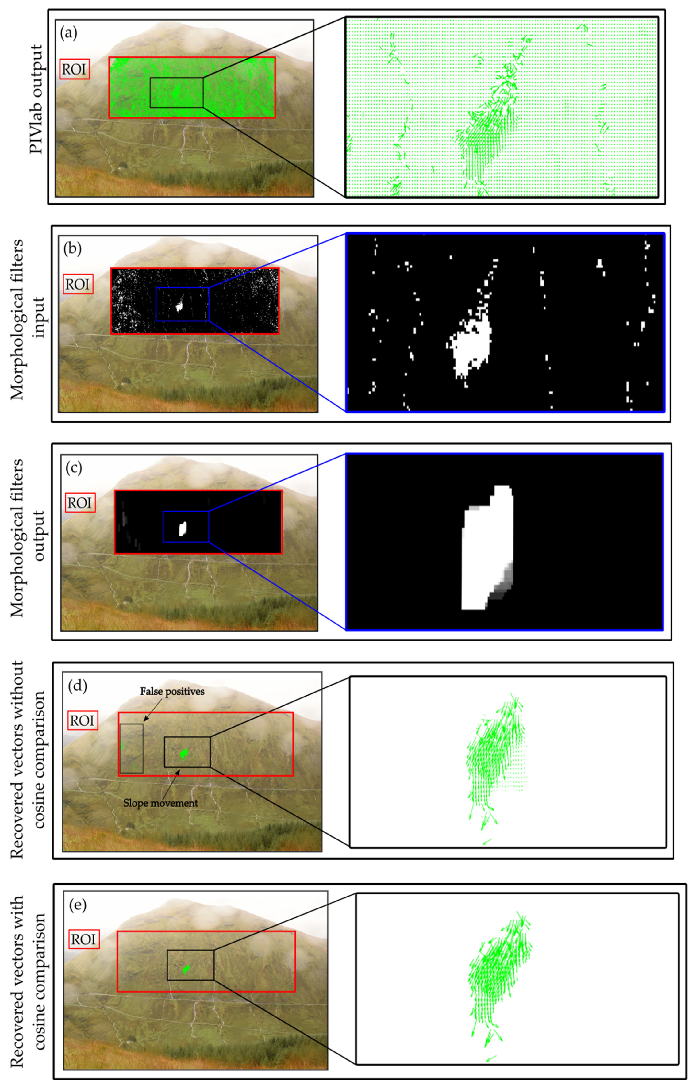
The refinement of PIVlab output via the morphological filtering and cosine comparison is demonstrated in Figure 8. The image interval was set to 24 h, thus one refined frame is generated after 48 h if cosine comparison is enabled. The image interval can be set to any desired value in the intervalometer settings. An initially ‘noisy’ frame is derived from PIV analysis of two images 24 h apart, containing vectors produced by water in gulleys and/or raindrops on the camera lens and genuine slope movement (a). The morphological filter inputs this noisy frame in a binary domain (b) and outputs a mask that covers only the area of genuine slope movement (c). This mask is superimposed on the original noisy frame (a), and only the vectors covered by this mask are restored (d). This process filters most of the noisy vectors however, a small number of false positives still remain in the frame. By cosine comparing the refined frame with the previous frame in the sequence one can effectively eliminate the false positives, as they do not appear in consecutive frames. The output frame of cosine comparator is shown in (e), where all but only genuine slope movement vectors are filtered out. As a result of filtering a small portion of vectors at the very edge of the genuine slope movement are also removed during the process. This can be avoided by increasing the dimension of ME. However, this comes at the cost of losing slope movements of small magnitudes completely, as they appear as small distance displacements and are treated as noise by the large dimension of ME.
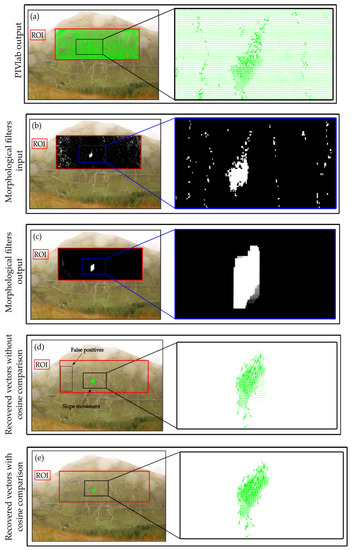
Figure 8.
Workflow of morphological filtering for vector frame refinement. (a) PIVlab output with image registration enabled and no filtering. (b) PIVlab output in binary domain, as input to first morphological filter (Erosion). (c) Output of second morphological filter (Dilation). (d) Recovered vectors from (b), when masked with the output of morphological filters (c). (e) Output of cosine comparator by analyzing two frames. Filter parameters: ME (4 × 2), : Rectangle, τ ≥ 0.8.
The remaining (proposed as ‘genuine’) slope movement vectors derived in this example relate to a failure that was also retrospectively identified and quantified with pre- (21 May 2018) and post-surveys (2 October 2018) using a Reigl VZ4000 terrestrial laser scanner. Terrestrial laser scans are subsampled to 0.2 m for change detection analysis between scans, and quantified the volume of displaced material at 187 m2 (Figure 9).
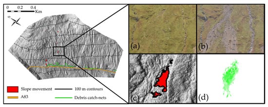
Figure 9.
(a) RGB-image pre slope failure, (b) RGB-image post slope failure, (c) terrestrial laser scanning derived digital elevation model of slope failure, (d) vectors from PIV capturing slope failure.
4. Automatic Landslide Detection: Monitoring Slope Failure Development
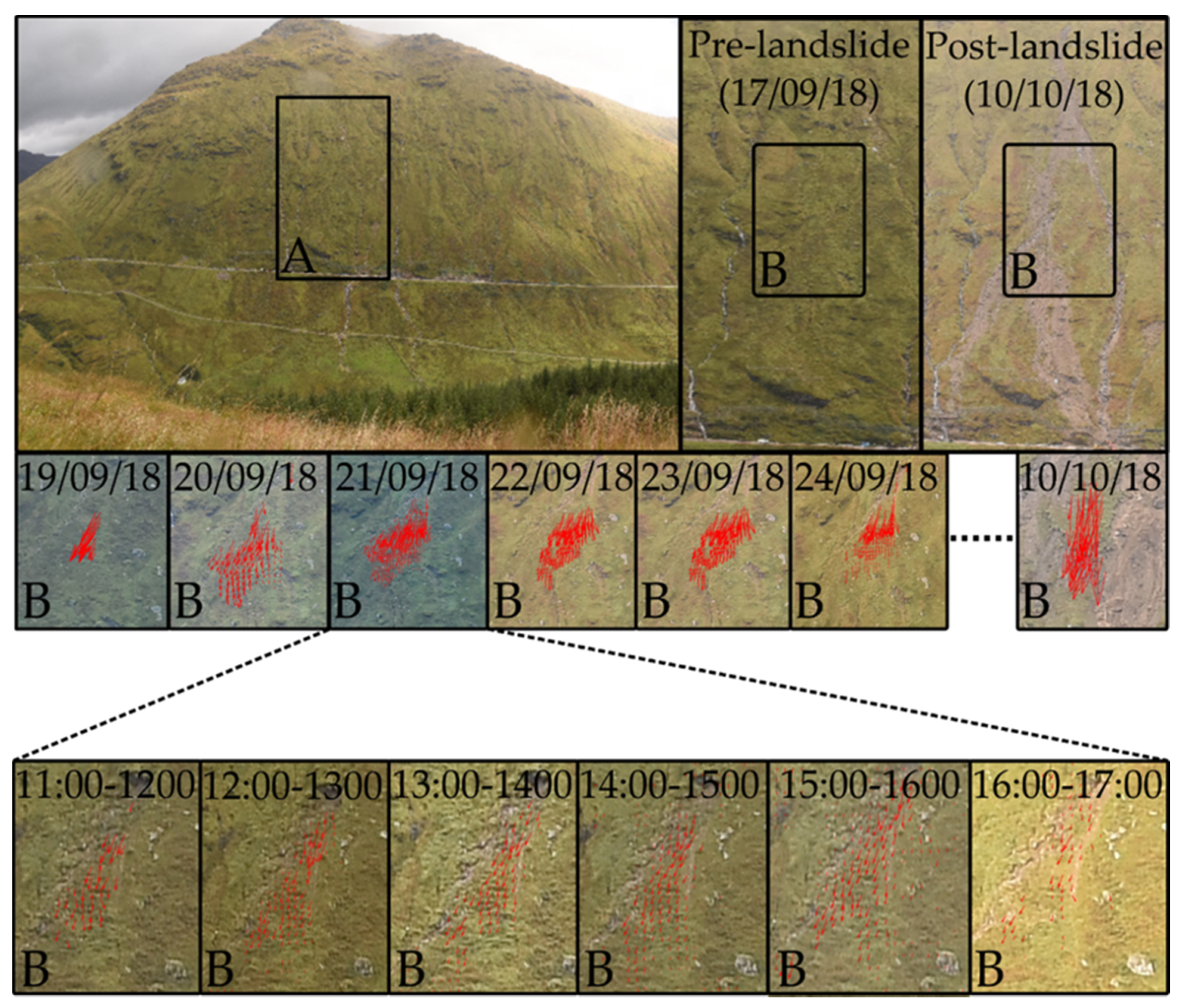
In September 2018, a slope creep landslide initiated as a response to rainfall from Storm Ali (a windstorm affecting the UK and Ireland in 2018). The TLI obtained over a period of 20 days prior to the landslide showed continuous creeping movement which is successfully detected by PIVlab. The movement is initially observed by PIVlab on the 19th of September 2018 which is followed by a series of TLIs with continuous movement detected. A sequence of TLIs are presented in Figure 10, which are obtained by processing two images 24 h apart and then by cosine comparing it with the last frame in the sequence. An hourly sequence of TLIs from the 21 September 2018 is also shown to demonstrate that movement was also detectable on shorter timescales. On the 9 October 2018 a debris-flow, sourced from higher up the Rest and Be Thankful slope, overran the observed creep movement (Figure 10–post-landslide).
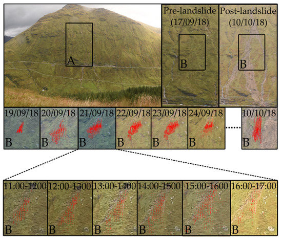
Figure 10.
Detection of creep landslide movement. (A) Pre and post failure TLI showing Rest and Be Thankful infrastructure. (B) Series of frames obtained by processing and filtering TLI, capturing slope movement. Filter parameters: ME (4 × 2), : Rectangle, τ ≥ 0.8.
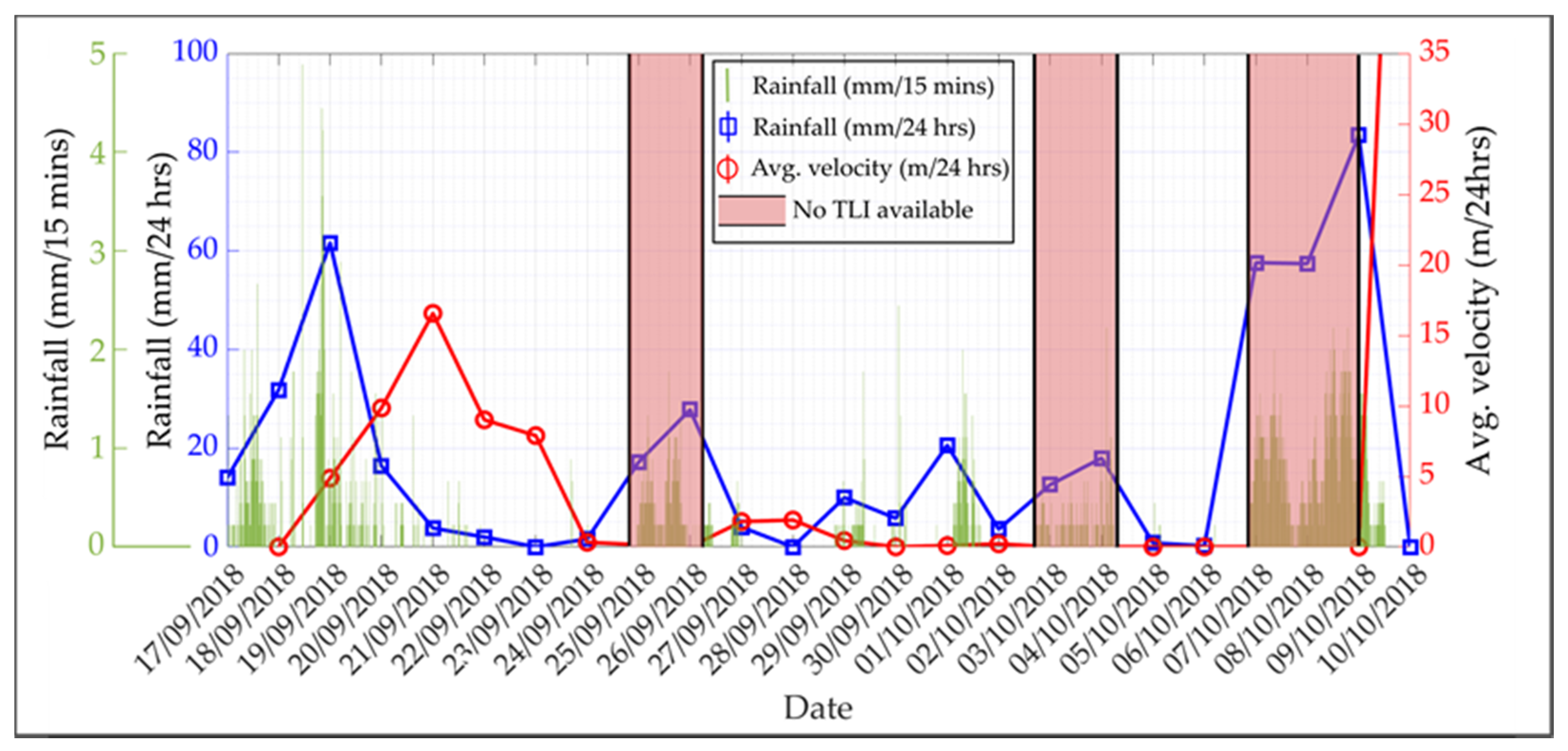
The initiation of the slope movement detected by PIV is correlated with peak rainfall (60 mm in the previous 24 h) from Storm Ali on the 19 September 2018; This is shown in Figure 11, which plots daily rainfall against the avg. velocity of movement recorded by PIVlab for a 24 h frequency of TLI. The velocity increases near linearly after initiation, despite the rainfall reducing. Peak velocity lags approximately 48 h behind peak rainfall then reduces to zero. From the Figure 11, it is also evident that the landslide does not respond strongly to subsequent rain events, and only rapidly accelerates after a second high-intensity rainfall event where 80 mm of rain is observed on the 9 October 2018. Two debris-flows sourced from the lower fringes of the movement on the 9 October 2018 but the main body of the creep movement did not transition to a debris-flow.
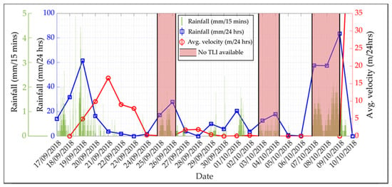
Figure 11.
Correlation between slope movement avg. velocity and rainfall observed from 17 September 2018 to 10 October 2018.
5. Discussion
The new additions to PIVlab presented here have enabled the effective detection of slope movement in real-time. This has been achieved using low-cost time-lapse camera hardware in a variety of harsh environmental conditions, across a wide (1 km) and morphologically complex slope. However, despite passing the data through a suite of filters, several challenges have been revealed through the application of these processes that merit further consideration. Here we discuss the success and potential of the remote, live-streamed system and image processing workflow for automated slope monitoring.
5.1. PIV Analyses in Dynamic Natural Environments
The effect of the uncontrolled and harsh environment was a major source of data corruption in the output of PIVlab. Uneven lighting and optical blocks such as clouds were mitigated by CLAHE and cloud detection algorithms, but occasional periods during which no useable images were captured due to low or poor visibility remained a constraint (Figure 11). These periods were induced by fog, raindrops on the camera lens, and poor lighting levels (Figure 12). The precursory movement observed before October 2018 landslide spanned 20 days, during which 512 images were captured out of which 193 were not processed due to poor visibility. Thus, for storm Ali, approximately 37% of the captured images were removed. Whenever features on the slope cannot be resolved across multiple images, PIV processing cannot identify and determine slope movements. However, it can be used to average the total movement throughout the recent monitoring period when the next clear image arrives. Despite missing some detail of the slope deformation stages, the total deformation and identification of movement across a selected ROI was not found to be significantly compromised.

Figure 12.
The effectiveness of TLI processing is limited by the occurrence of foggy conditions, raindrops on the camera lens, and low lighting.
The number of false-positives were reduced significantly by introducing erosion and dilation filters, and by applying a cosine comparator. A small number of false-positive were still detected and these were eliminated by increasing the size of ME during the morphological filtering. However, this process limits the detection of small slope movements and only movements of considerable amplitude would be detected. It should also be noted that the approach has performed well in poor visibility conditions because it compares new images with the last ‘usable’ (defined by κ) rather than the previously captured image when poor conditions lead to multiple rejected images. Although it could theoretically detect events when the slope is snow covered, no such events have occurred during monitoring.
5.2. Recommendations for Optimizing PIV Analyses for Slope Monitoring Applications
The resolution of the optical sensor puts a constraint on how well the PIV analysis detects a slope movement. Detecting change across a wide and varied slope requires a high-resolution camera, with sufficient field of view to cover the wide area and yet still resolve features consistently. With a lower resolution optical sensor, small slope movements, such as those associated with the initial development of a slope failure, would go undetected. With the camera setup used in this study, one pixel covers 0.61 m2 of slope. Thus, any movement observed between two images with magnitude less than 0.61 m will go undetected. This limitation can be countered by increasing the resolution of the optical sensor, or a different lens setup depending on the region of interest. It is, therefore, necessary that the system achieves a balance between coverage and detail on the slope from a suitable vantage point, ideally positioned face-on to the monitored slope.
The temporal resolution or framerate plays an important role in the PIV outputs generated. A higher framerate is desired in order to minimize the differences between images but for real-time monitoring the data telemetry and processing time required to generate a difference frame must be considered. For landslide detection using TLI, a high framerate provides high sensitivity to the detection of movement, but where events take several hours to days to fully develop lower capture rates can still prove successful, albeit with a loss of granularity in the temporal component of deformation.
5.3. The Potential for PIV Analyses for Slope Monitoring
Through the application of the processing workflow, initial precursory movement and landslide inception at our case-study site was detected during a rainfall event approximately 20 days before the ultimate failure. Despite being limited to conditions where the features of the slope are visible, the ability to monitor and automatically detect movements across an expansive and complex slope area using low-cost hardware holds significant potential to improve the accurate detection and forecasting of damaging landslides. In many situations, landslides can typically only be loosely linked to driving processes by the final time failure or interaction with assets. Our approach has the potential to help better constrain the timing, evolution, and magnitude of slope failures relative to triggering events.
Live-streamed and automated movement data enable the creation and analysis of an inventory of change on problematic slopes that can improve assessment of instabilities that may ultimately threaten key assets or pose risk to life. The PIV analyses have detected the initiation, development, and the reactivation of slope material prior to final failure in a challenging slope setting. Further analysis may help asset managers to better understand the types of movement that develop into potentially hazardous events and those that do not. Ultimately this new approach will enable a move away from retrospectively identifying where individual events may have initiated to proactively tracking and mitigating threats as they develop.
6. Conclusions
A real-time landslide monitoring solution has been presented by employing PIV, a powerful fluid visualization technique that works on the principles of cross-correlation between images. The approach has been developed and applied at a problematic site where landslides repeatedly threaten the operation of the A83 in Scotland. We use live-streamed TLI, which require pre-processing for contrast equalization, intensity thresholding, and image registration to account for low or variable (contrast) light levels, windy conditions, and raindrops on the camera lens. The output velocity vectors obtained by cross-correlating the enhanced pre-processed TLI via PIV were passed through a chain of filters to distinguish false positives from the vectors generated by the actual slope movement. These include a pair of morphological filters, applied to the output of PIV in the visual domain. This procedure was followed by allowing the refined vector set to pass through a comparator, where vectors from two consecutive PIV outputs were matched for similarities in terms of the angle between them. This addition was deemed essential in order to identify vectors produced by genuine slope movements, which produced higher gradient similarity values. We demonstrate that the final product achieved represents an effective, low-cost approach to automatic detection of slope movement and provides a powerful new early warning tool to mitigate the impacts of landslides affecting critical assets.
Author Contributions
The authors contributions are as follows: The article and new elements of the code were written by M.W.K., R.B., S.D., M.L. and J.M. conceptualized the idea of slope movement detection via particle image velocimetry. R.B. and A.D.-M. set up the hardware for data collection, M.L., S.D., J.M., H.T., N.J. and J.W. reviewed and supervised the project work and the manuscript development. All authors have read and agreed to the published version of the manuscript.
Funding
NERC grants NE/P000010/1; NE/T005653/1 and NE/T00567X/1 and a Scottish Roads Research Board (SRRB) award ‘Innovative monitoring strategies for managing hazardous slopes’.
Acknowledgments
The authors gratefully acknowledge the support of Transport Scotland, BEAR, Geo-Rope and Jacobs. We are thankful to William Thielicke for providing PIVlab as an open source software to be used by the wider research community.
Conflicts of Interest
The authors declare no conflict of interest.
Abbreviations
| PIV | Particle Image Velocimetry |
| TLI | Time Lapsed Images |
| IA | Interrogation Area |
| CLAHE | Contrast Limited Adaptive Histogram Equalization |
| ME | Morphological Element |
| ROI | Region Of Interest |
| DSLR | Digital Single-Lens Reflex |
| LiPo | Lithium Polymer |
| FFT | Fast-Fourier Transform |
| iDFT | Inverse-Discrete Fourier Transform |
References
- Garianoab, S.L.; Guzzetti, F. Landslides in a changing climate. Earth Sci. Rev. 2016, 162, 227–252. [Google Scholar] [CrossRef]
- Reder, A.; Rianna, G.; Mercogliano, P.; Pagano, L. Assessing the potential effects of climate changes on landslide phenomena affecting pyroclastic covers in Nocera area (Southern Italy). Procedia Earth Planet. Sci. 2016, 16, 166–176. [Google Scholar] [CrossRef]
- Williams, J.; Rosser, N.J.; Afana, A.; Hunter, G. Can full-waveform of terrestrial laser scanning enhance our ability to monitor rock slope failure? In Proceedings of the 2013 International Symposium on Slope Stability in Open Pit Mining and Civil Engineering, Brisbane, Australia, 25–27 September 2013. [Google Scholar]
- Carlà, T.; Tofani, V.; Lombardi, L.; Raspini, F.; Bianchini, S.; Bertolo, D.; Thuegaz, P.; Casagli, N. Combination of GNSS, satellite InSAR, and GBInSAR remote sensing monitoring to improve the understanding of a large landslide in high alpine environment. Geomorphology 2019, 335, 62–75. [Google Scholar] [CrossRef]
- Pratesi, F.; Nolesini, T.; Bianchini, S.; Leva, D.; Lombardi, L.; Fanti, R.; Casagli, N. Early warning GBInSAR-based method for monitoring Volterra (Tuscany, Italy) city walls. IEEE J. Sel. Top. Appl. Earth Obs. Remote Sens. 2015, 8, 1753–1762. [Google Scholar] [CrossRef]
- Mayinger, F.; Feldmann, O. Optical Measurements. Techniques and Applications. In Optical Measurements: Techniques and Applications; Springer: Berlin/Heidelberg, Germany, 2001; pp. 337–353. [Google Scholar]
- Winter, M.; Peeling, D.; Palmer, D.; Peeling, J. Economic impacts of landslides and floods on a road network. AUC Geogr. 2012, 54, 207–220. [Google Scholar] [CrossRef]
- Finlayson, A. Glacial conditioning and paraglacial sediment reworking in Glen Croe (the Rest and be Thankful), western Scotland. Proc. Geol. Assoc. 2020, 131, 138–154. [Google Scholar] [CrossRef]
- Sparkes, B.; Dunning, S.; Lim, M.; Winter, M.G. Characterisation of Recent Debris Flow Activity at the Rest and Be Thankful, Scotland; Advancing Culture of Living with Landslides; Workshop on World Landslide Forum: Ljubljana, Slovania, 2017. [Google Scholar]
- Brennen, C. Fundamentals of Multiphase Flow; Cambridge University Press: Cambridge, UK, 2005. [Google Scholar]
- Huang, H.; Dabiri, D.; Gharib, M. On the errors of digital particle image velocimetry. Meas. Sci. Technol. 1997, 8, 1427–1440. [Google Scholar] [CrossRef]
- Thielicke, W. The Flapping Flight of Birds: Analysis and Application. Ph.D. Thesis, University of Groningen, Groningen, The Netherland, 2014. [Google Scholar]
- Okamoto, K.; Nishio, S.; Saga, T.; Kobayashi, T. Standard images for particle-image velocimetry. Meas. Sci. Technol. 2002, 11, 685. [Google Scholar] [CrossRef]
- Stamhuis, E.J. Basics and principles of particle image velocimetry (PIV) for mapping biogenic and biologically relevant flows. Aquat. Ecol. 2016, 40, 463–479. [Google Scholar] [CrossRef]
- Keane, R.; Adrian, R. Theory of cross-correlation analysis of PIV images. Appl. Sci. Res. 1992, 49, 191–215. [Google Scholar] [CrossRef]
- Thielicke, W.; Stamhuis, E.J. PIVlab—Towards user-friendly, affordable and accurate digital particle image velocimetry in MATLAB. J. Open Res. Softw. 2014, 2. [Google Scholar] [CrossRef]
- Pizer, S.M.; Amburn, E.P.; Austin, J.D.; Cromartie, R.; Geselowitz, A.; Greer, T.; ter Haar Romeny, B.; Zimmerman, J.B.; Zuiderveld, K. Adaptive histogram equalization and its variations. Comput. Vis. Graph. Image Process. 1987, 39, 355–368. [Google Scholar] [CrossRef]
- Shavit, U.; Lowe, R.; Steinbuck, J. Intensity Capping: A simple method to improve cross-correlation PIV results. Exp. Fluids 2007, 42, 225–240. [Google Scholar] [CrossRef]
- Maragos, P. The Essential Guide to Image Processing; Chapter 3: Morphological filters; Academic Press: Cambridge, MA, USA, 2009; pp. 293–321. [Google Scholar]
Publisher’s Note: MDPI stays neutral with regard to jurisdictional claims in published maps and institutional affiliations. |
© 2021 by the authors. Licensee MDPI, Basel, Switzerland. This article is an open access article distributed under the terms and conditions of the Creative Commons Attribution (CC BY) license (http://creativecommons.org/licenses/by/4.0/).


