Sentinel-1 Big Data Processing with P-SBAS InSAR in the Geohazards Exploitation Platform: An Experiment on Coastal Land Subsidence and Landslides in Italy

Abstract

The growing volume of synthetic aperture radar (SAR) imagery acquired by satellite constellations creates novel opportunities and opens new challenges for interferometric SAR (InSAR) applications to observe Earth’s surface processes and geohazards. In this paper, the Parallel Small BAseline Subset (P-SBAS) advanced InSAR processing chain running on the Geohazards Exploitation Platform (GEP) is trialed to process two unprecedentedly big stacks of Copernicus Sentinel-1 C-band SAR images acquired in 2014–2020 over a coastal study area in southern Italy, including 296 and 283 scenes in ascending and descending mode, respectively. Each stack was processed in the GEP in less than 3 days, from input SAR data retrieval via repositories, up to generation of the output P-SBAS datasets of coherent targets and their displacement histories. Use-cases of long-term monitoring of land subsidence at the Capo Colonna promontory (up −2.3 cm/year vertical and −1.0 cm/year east–west rate), slow-moving landslides and erosion landforms, and deformation at modern coastal protection infrastructure in the city of Crotone are used to: (i) showcase the type and precision of deformation products outputting from P-SBAS processing of big data, and the derivable key information to support value-adding and geological interpretation; and (ii) discuss potential and challenges of big data processing using cloud/grid infrastructure.

1. Introduction

The last three decades have witnessed the increasing and widespread use of satellite synthetic aperture radar (SAR) imagery to retrieve key information on surface deformation processes affecting the Earth’s surface using two- and three-pass differential interferometric SAR (InSAR) (e.g., [1,2,3]), and multi-pass/multi-temporal InSAR methods, such as persistent scatterers interferometry (PSI) (e.g., [4,5]) and Small BAseline Subset (SBAS) (e.g., [6,7]). Many SAR constellations have been developed since the 1990s and, as part of their background observation scenarios, have been tasked to acquire images regularly over major cities, targets with economic and/or strategic relevance (e.g., key infrastructure, polar regions, cultural heritage sites), regions affected by specific Earth hazards (e.g., tectonic zones and volcanoes), and entire nations or continents (e.g., [8,9]).

This means that the volume of SAR data collected to date, archived, and available for InSAR applications by far falls within the “big data” remit for such type of imagery (typically, 15–20 SAR scenes are needed as minimum input of an advanced InSAR analysis, e.g., [5], and usually a few to several tens of scenes are used in most InSAR applications), thus creating novel opportunities and opening new challenges for Earth sciences and observation (e.g., [10,11]). For instance, since the beginning of its operations in late 2014, the Copernicus Sentinel-1 SAR constellation acquired over each area of Europe around 300 passes for each geometry, i.e., ascending and descending, with an initial repeat pass of 12 days with Sentinel-1A only (~180 scenes in 6 years), which was improved to 6 days in late 2016 thanks to the addition of Sentinel-1B to the constellation (another ~120 scenes in 4 years). This can be verified by consulting the ESA Copernicus Open Access Hub [12].

Thus, researchers willing to undertake multi-temporal InSAR studies of long-term (e.g., more than 3–5 years) dynamics of deformation processes face two main challenges. First, they need to find efficient combinations of computing infrastructure, algorithms, and software capable to run and optimize the big SAR data processing workflow. Second, they need to use tools to handle and analyze the outputs of such processing, which (proportionally to the processed area extent and its land cover) may consist of hundreds of thousands or millions of persistent or coherent targets, each equipped with information of geolocation, quality, annual displacement velocity, and a full deformation record, the length of which depends on the number of input SAR scenes processed.

Parallelized InSAR processing chains running on cloud and grid computing infrastructure help to address the first challenge. They relieve researchers of demanding tasks for big data download and processing in local PCs, and drastically reduce processing times (e.g., [13,14]). On the other side, InSAR dataset screening approaches and statistical methods to detect outliers, trend changes, accelerations/decelerations, and other deviations from the expected deformation behavior contribute to addressing the second challenge [15,16,17,18].

In this respect, the present study has three main goals:

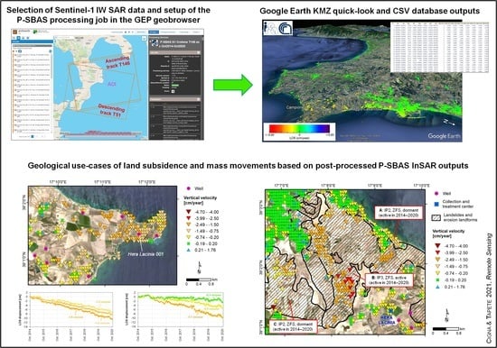
• First, to demonstrate that through parallelized InSAR processing chains running on data exploitation platforms, it is possible to process big SAR time series made of an unprecedented number of Sentinel-1 images, i.e., in the order of hundreds per single observation geometry.
• Second, to showcase that big InSAR datasets can be generated across geographic areas of either urban or rural land cover (or a mixture of them), and later be post-processed to derive value-added products. These InSAR datasets are as “big” in the time-domain as the amount of input SAR images, and therefore as the number of observations composing the deformation time series of each persistent or coherent target obtained at the end of the multi-interferogram processing. Furthermore, they are “big” in the space-domain on the basis of the total number of persistent or coherent targets themselves that the interferogram network created during InSAR processing has allowed to identify over the long time span investigated (despite the relatively small region of interest of this work).
• Third, to prove that such big InSAR datasets can be handled through post-processing and data integration methodologies that have been established by the geohazard community in the last decade, and be transformed into higher-level geospatial information to characterize geological hazards of potential concern of local stakeholders. Without claiming to fully develop specific user-oriented or user-driven applications, this paper does not restrict to the presentation of InSAR results only (which is the dominant feature of most of the published literature on InSAR processing using cloud/grid computing), but also encompasses selected use-cases of geological interpretation.

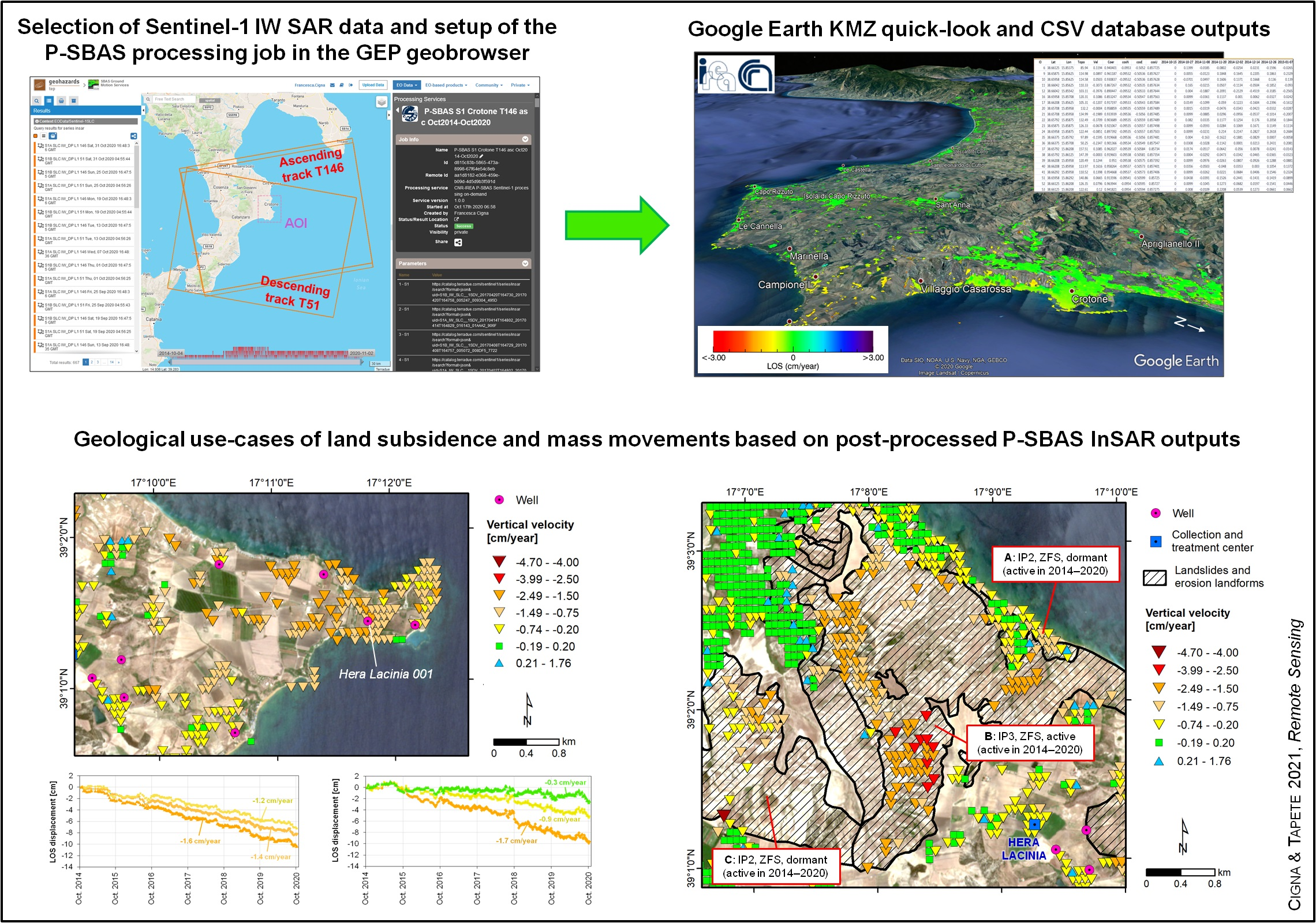
To address the first two aims, in this study, six full years of Sentinel-1 SAR ascending and descending mode imagery compose the big data volume used as input. Multi-temporal InSAR processing was carried out using the parallelized implementation of the SBAS differential InSAR approach, also referred to as Parallel-SBAS (P-SBAS) [19], which was developed at the Institute for Electromagnetic Sensing of the Environment (IREA) of the National Research Council (CNR) of Italy and integrated in the European Space Agency (ESA)’s Geohazards Exploitation Platform (GEP). The latter is a cloud-based environment sourced with data (both optical and SAR), tools, and processing services, aimed to support satellite Earth observation (EO) exploitation for geohazards [20]. Developed as an ESA Thematic Exploitation Platform (TEP) in 2015, and conducted by a consortium led by Terradue Srl, the GEP follows the SuperSites Exploitation Platform (SSEP), which was originally initiated in the context of the Geohazard Supersites and Natural Laboratories initiative. Over the years, the platform has expanded to address broader objectives of the geohazards community, including several activities and projects of the Committee on Earth Observation Satellites (CEOS) Working Group on Disasters [21]. The GEP is now used by a large community of researchers and stakeholders working in the field of EO, with a focus on mapping hazard-prone areas and monitoring terrain deformation. Information on how to access the GEP and exploit its on-demand and systematic services is available on the dedicated website (https://geohazards-tep.eu), along with a description of all thematic apps, services, datasets, and other resources.

To the best of our knowledge, the present big data processing experiment with P-SBAS is the one exploiting the longest-ever Sentinel-1 SAR interferometric stacks used so far for a single study site, not only among the studies employing the P-SBAS method, but also globally, as the longest Sentinel-1 stacks published in the literature consisted of no more than 140–190 acquisitions each (e.g., [22,23,24]) or up to 240–260 (e.g., [25]). Therefore, in terms of the size of the input SAR data stack processed, this study aspires to act as a pioneering proof-of-concept of big SAR data analysis with multi-interferogram algorithms, and in particular the P-SBAS implementation.

Compared to the more paroxystic and catastrophic hazards that are commonly observed with the GEP (e.g., floods and tectonic deformation), this study focuses on more “silent” and subtle hazards, i.e., slow-moving landslides and coastal subsidence, whose regular monitoring and early-stage characterization could provide evidence-based input into land management, land-use planning, and environmental assessments. For this purpose, a coastal study area in southern Italy (Figure 1) was selected to include the city of Crotone and its province, the Capo Colonna promontory and the namesake archaeological site in Calabria Region, where ground instability, including both natural geological processes and human-induced hazards, have been recorded (e.g., [26,27,28]). Instances of surface deformation matching with known landslides, long-term subsidence, and modern coastal protection infrastructure are used to showcase the type and precision of deformation products that can be generated with P-SBAS processing of Sentinel-1 big data using the GEP, and also the key information retrievable to support the geological interpretation and analysis of the process under investigation. This includes value-adding through the combination of multiple P-SBAS datasets for the retrieval of the vertical and east–west deformation fields (Section 5.1), and discussion of the geo-information and knowledge enhancement through ground deformation datasets outputted from a SAR big data analysis (Section 5.2).

2. Study Area

The study area in Calabria Region, southern Italy, extends 300 km² across the Crotone Basin (Figure 1), which lies on the Ionian side of the Calabrian Arc, i.e., one of the highly active Mediterranean tectonic regions. From a geological point of view, the basin is generally considered a fore-arc basin [31]. It started opening between Serravallian and Tortonian, on top of the SE verging Calabrian accretionary wedge, the latter being grown along the Neogene subduction zone between the sinking Ionian lithosphere and the overriding European plate [32]. Two NW-trending sinistral shear zones laterally bound the basin [31]. According to the model proposed by Van Dijk [33], such basement wrench faults caused the partitioning of the basin into separate sub-basins subject to differential subsidence and mutual displacements [34].

Along the coasts of the Crotone province, several marine terraces nowadays provide the evidence of the strong uplift that affected the Calabrian Arc since the Middle Pleistocene. At these terraces, a transgressive erosional surface can be recognized, above which shallow-marine sediments unconformably overlie a Plio-Pleistocene slope succession known as the Cutro Clay [31]. In absence of a general consensus on their number and identification [31], and following the identification made by Zecchin et al. [35], these marine terraces are referred to as (Figure 1c): the older Cutro terrace (1st order, Middle Pleistocene) and the Late Pleistocene Campolongo (2nd order), Capo Cimiti (3rd order), Capo Rizzuto (4th order) and Le Castella (5th order) terraces [30,36]. Being placed at progressively lower elevations (around 180–200 m a.s.l.) and dislocated by Quaternary faults [31], these terraces are a distinctive feature of the local topography (Figure 1b).

Of these, it is worth focusing on the terrace a few kilometers SE from Crotone that occupies the 3 km EW-elongated promontory of Capo Colonna (Figure 1b), i.e., the easternmost piece of land in the study area, projecting into the Ionian Sea with an eastward dip of ~1° [31]. A topographic gradient characterizes the promontory, from ~50 m a.s.l. elevation at the N-trending landward border representing a paleo-coastline, up to 10-15 m a.s.l. at the coastal cliffs [31]. The internal margin of the terrace is covered by a colluvial layer, while seaward up to 10 m thick carbonate and siliciclastic sediments are found. This complex sedimentary body exhibits a non-homogeneous behavior, from both hydrogeological and mechanical points of view [37].

While in other terraces the steep cliffs are carved in terrace deposits, at Capo Colonna they are carved directly into older units [38] and are subject to severe marine erosion due to strong wind-driven waves undercutting the newly exposed base of the cliffs. Large slabs of Pleistocene fossiliferous calcarenite consequentially fall down [27], thus contributing to severe scarp retreat that threatens the structural stability of properties and the preservation of renown archaeological monuments located close to the cliff edge [27,37,39].

Coastal erosion has been affecting this area for centuries, together with subsidence and tectonic-induced submergence of sites that were once sub-aerially exposed along the coast. Zecchin [40] has demonstrated the relationship between such fault-controlled subsidence and preservation of shallow-marine small-scale cycles visible in the northern Crotone Basin. More south in our study area, Stanley and Bernasconi [27] and the studies that they reviewed have demonstrated that the positions of modern Calabrian shorelines considerably differ from the former in Greek and early Roman times, with a landward retreat in the order of 200 m. Several sites submerged due to a number of tectonic pulses over time. Excluding world (eustatic) sea-level rise, Stanley and Bernasconi [27] estimate that during the past ~3000 years in the late Holocene, subsidence has ranged from ~0.5 mm/year to the remarkably high value of ~4 mm/year.

At present, other factors that may cause land subsidence and surface ground deformation across the region are not only hotspots of groundwater pumping for local agricultural and industrial activities, but also hydrocarbon exploitation [41].

The Crotone Basin and its offshore expansion have been extensively investigated for oil exploration [32]. Natural gas seepages were discovered in Cutro and Isola Capo Rizzuto, while a group of fields with thermogenic gas is located offshore of Capo Colonna (Figure 1b) [42]. The Luna–Hera Lacinia–Linda field (1971, gas 370–400 million barrels of oil equivalent) is indeed among the several offshore fields discovered in Italy during the decade 1965–1974, and has been attributed to the Tertiary Supercycle–Oligocene-Miocene thermogenic gas petroleum system family [43].

Figure 1b shows the location of hydrocarbon production infrastructure and concession areas as per the Italian Ministry of Economic Development’s database [29]. For the purposes of interpretation of the ground motions found in the Sentinel-1 data InSAR processing (see Section 4), it is worth focusing on the concession area called “Capo Colonne,” which extends nearly 65 km² over the southern part of the Crotone province and encompasses the namesake promontory. Granted on September 1997 for 30 years, and once renewed in 2007 for additional 10 years, “Capo Colonne” has recently been operated by Ionica Gas, and then by the national hydrocarbons authority ENI (Ente Nazionale Idrocarburi), and includes the Hera Lacinia collection and treatment center (Figure 1b), as well as the production well Hera Lacinia 001 [29].

The potential impact of such exploitation activities on ground stability and local anthropogenic assets has been assessed based on an ad hoc geodetic–geophysical monitoring network installed in 2005 in the Archaeological Park of Capo Colonna, in the framework of a collaboration between ENI Spa E&P Division and the Superintendence for Archaeological Heritage of Calabria [37]. This integrated system included satellite SAR surveys among the shallow monitoring techniques employed by ENI in their typical subsidence monitoring networks [44]. SAR was also used in research papers for high-resolution [45] and multi-temporal [46,47] assessment of land subsidence in the last 25 years.

InSAR was helpful to investigate landslides that are distributed across the Crotone province and update their inventory [48]. Through integration with seismic profiles, morpho-bathymetric and GPS data, InSAR was brought among the evidence to support the discussion on the existence of a large-scale gravitational megalandslide off the Crotone Basin [28].

Limiting to inland susceptibility to landslides, which is one of the geological focuses of the present study, it is worth recalling that in the central and southern parts of the Crotone province hill-slopes carved into clayey and marly–clayey deposits are subject to slope-wash processes (sheet, rill, and gully flow), and lead to the development of erosion landforms called “calanchi” (i.e., a type of badland formed in clayey bedrock) [49]. These landforms are found in the coastal area south of Crotone; for instance, between the settlements of Vrica and Semaforo, and more inland toward Farina IV and Trafinello (Figure 2).

3. Materials and Methods

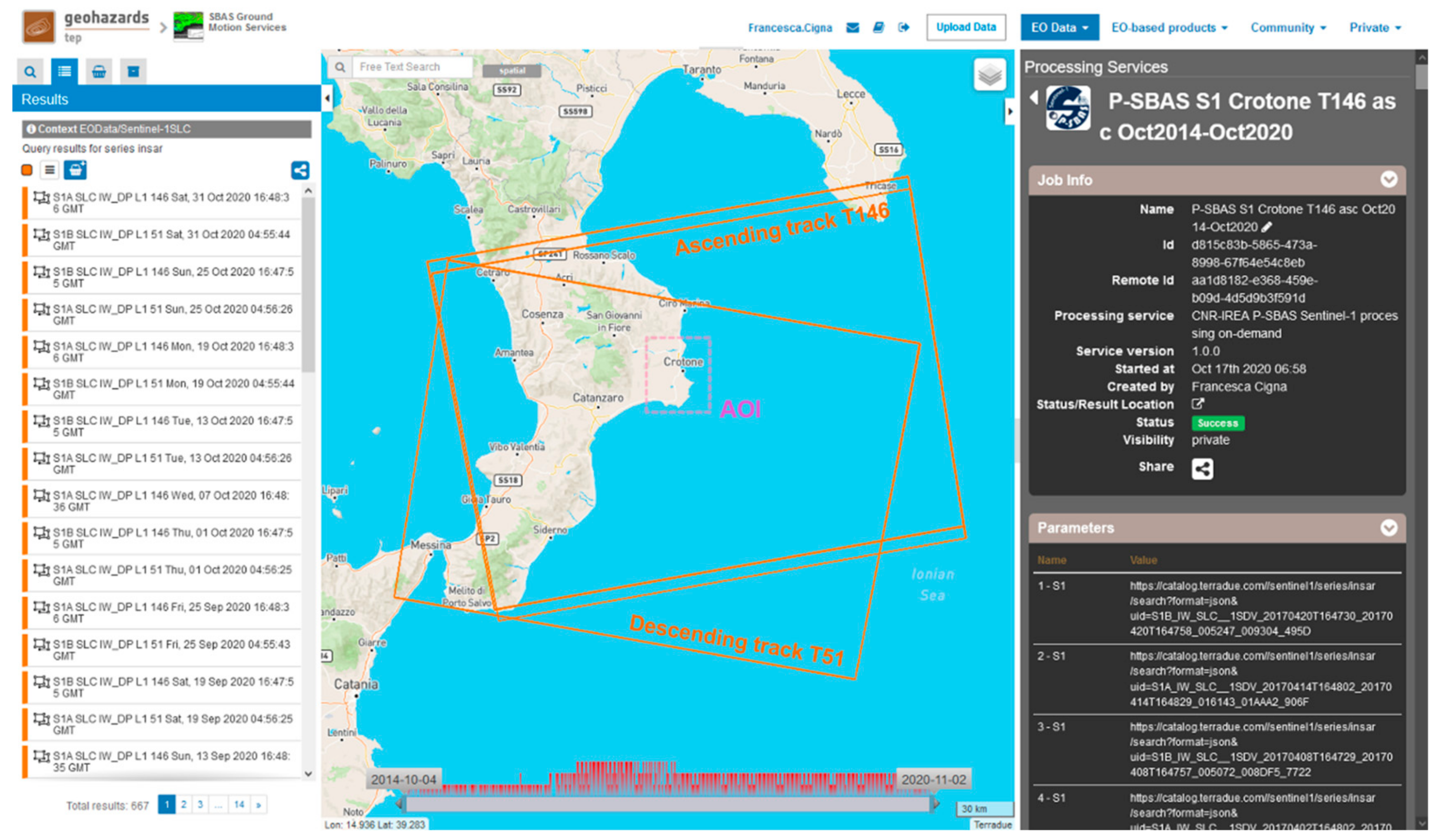
3.1. Input SAR Data

A total of 579 Sentinel-1 SAR scenes were used for the analysis. These were acquired by the radar sensors operating in C-band (5.405 GHz central frequency f, and 5.547 cm wavelength λ) onboard the two satellites Sentinel-1A (launched on 3 April 2014) and Sentinel-1B (launched on 25 April 2016), which are phased at 180° to each other along the same near polar, sun-synchronous orbit at ~693 km altitude [50].

The data were acquired in right-looking mode over a 6 year-long period between October 2014 and October 2020, along ascending track T146 (296 scenes: 15 October 2014–13 October 2020, acquired at 18:48 local time) and descending track T51 (283 scenes: 21 October 2014–13 October 2020, at 06:55 local time). The spatial footprints of the two data stacks are shown in Figure 1a and, with zoomed view, in Figure 3. As per the mission observation scenario over Europe [9], until September 2016, the site revisit at the study area was of 12 days (for each geometry), while an improvement to 6 days was later achieved thanks to the addition of Sentinel-1B. This means that each data stack consists of an image every 12 days in the period October 2014–September 2016, and every 6 days in September 2016–October 2020. The frequency distribution of the available scenes along both tracks is shown in the time-bar in Figure 3. All scenes acquired in the period October 2014–October 2020 were used for the analysis.

The employed acquisition mode was the Interferometric Wide (IW) swath, which is based on the Terrain Observation with Progressive Scans (TOPS) ScanSAR mode [51]. The IW swath width was 250 km, and the incidence angle θ of the line-of-sight (LOS) varied between 31° and 46° from the near to the far range (i.e., ~39° at scene center). The pixel spacing was 2.3 m in slant range and 14.1 m azimuth, resulting in ground range and azimuth resolution of 5 m and 20 m (single-look), respectively.

The IW scenes were accessed through the GEP as Level-1 Single Look Complex (SLC) data (Figure 3), consisting of focused SAR products in zero-Doppler slant-range geometry, georeferenced using satellite orbit and attitude data.

While Sentinel-1 IW data were acquired with dual polarization (co-polarized VV and cross-polarized VH), for this study the VV imagery was selected to run the P-SBAS processing, with the aim to guarantee continuity with previous co-polarization InSAR studies over the same region (see Section 5.1.1). Future research on this area will also attempt the exploitation of the VH data, both for comparison and in combination with VV. While the use of the VH data alone provides lower performance in terms of candidates and final persistent targets identification due to the generally lower amplitude of cross-polarized imagery (e.g., [52]), their combined exploitation with VV data through optimization methods proved capable to enhance the performance (e.g., [52,53]). This could be a way forward for future research specifically aiming to compare the InSAR processing performance and accuracy at different polarizations.

3.2. P-SBAS InSAR Processing

The multi-interferogram processing was executed in ESA’s GEP by exploiting the “CNR-IREA P-SBAS Sentinel-1 processing on-demand” service v.1.0.0 within the “CNR-IREA SBAS Ground Motion Services” Thematic App (Figure 3). The processing approach builds upon the SBAS technique [6], and has been adapted to efficiently run on high-performance distributed-computing infrastructure (e.g., grid and cloud computing) [13], and tailored for Sentinel-1 IW TOPS data processing [54].

Since its development in early 2010s, a huge number of experiments and test-cases have been run with P-SBAS by the developers team at CNR-IREA (e.g., [13,19,54,55,56,57,58,59]), as well as by independent research teams in the GEP Early Adopters Programme (e.g., [23,24,60,61,62,63,64,65,66,67,68,69]), using ERS-1/2, ENVISAT, COSMO-SkyMed, and Sentinel-1 SAR imagery. Not only local and city scale, but also regional (e.g., [13,57,58,65]), national (i.e., Italy; [54,59]), and up to continental (i.e., whole Europe; [22]) scale studies have been successfully carried out. Moreover, different computing infrastructure setups have been trialed for the data processing, including CNR-IREA’s own cluster (e.g., [19,56,57,70]), the Amazon Web Services (AWS) cloud-computing environment (e.g., [13,54,56,57,58]), ESA’s Grid-Processing On Demand (G-POD) (e.g., [55,60,65,68,69,71,72]) and GEP (e.g., [24,61,63,64,67]), and more recently the ONDA Data and Information Access Service (DIAS) [22].

In this framework, the published literature shows a yet relatively limited number of applications that aimed to exploit this service for geological investigations (e.g., [23,24,61,63,64]), since the release of the P-SBAS Sentinel-1 on-demand service within the GEP in early 2019. Therefore, this study also contributes to this research direction.

The processing in GEP began with the retrieval of the input SLC data from the image archives, which is mainly based on the repositories of the ESA Open Access Hub, ONDA DIAS, and CREODIAS. Each SLC data stack was co-registered at the single-burst level ensuring very high coregistration accuracy (in the order of 1/1000 of the azimuth pixel size), as required for TOPS data due to the large along-track Doppler centroid variations [73]. Small temporal and perpendicular baseline pairs were selected to form the interferograms, with the aim to reduce interferometric phase decorrelation [74] by limiting the maximum number of consecutive acquisitions to be used to form the pairs [54], and by exploiting the narrow orbital tube (i.e., 100 m diameter during nominal mode operations; [50]).

A complex multi-looking operation in azimuth and range (5 by 20) was applied to mitigate the decorrelation noise in the interferograms and generate the coherence maps, thus reaching ground pixel spacing of ~90 m, as per the default parameter setting of the current P-SBAS service version in the GEP. Topographic phase components were derived and subtracted based on NASA’s 1 arcsec (i.e., 30 m) resolution Shuttle Radar Topography Mission (SRTM) Digital Surface Model (DSM). Multi-looked burst interferograms were mosaicked to sub-swaths, and then the two sub-swaths covering areas of land were mosaicked together to reach two-thirds of the swath. i.e., ~170 km (see stack coverage in Figure 3). The interferograms were then noise-filtered using the Goldstein filter with 0.5 weight [75], and optimized triangular networks of interferograms were identified [76], including 861 interferograms for the ascending stack, and 828 for the descending stack. Temporal and spatial phase-unwrapping was implemented with the extended minimum cost flow (EMCF) algorithm [77]. Across the large expanses of rural and vegetated land in the northwestern sector of the processed region, the phase-unwrapping step was more challenging, as typically happens across these land cover types, where errors are more likely to occur due to widespread phase decorrelation.

Least square solution retrieval was used for coherent targets using the singular value decomposition (SVD) method, and residual orbital ramps were estimated (as the linear components of phase artifacts; [78]) and then removed from the wrapped interferograms [19]. A second iteration of temporal and spatial phase-unwrapping was implemented for the orbit error-free interferograms, followed by SVD, as per the P-SBAS Sentinel-1 workflow [54]. Temporal coherence was computed, and the threshold on the minimum allowed temporal coherence to select coherent targets was set at 0.85. Atmospheric phase components were identified and removed. The output datasets including geolocation (i.e., latitude and longitude in the WGS84 system, and elevation above the reference ellipsoid), annual LOS velocity, and date-by-date displacement histories (time series) for each coherent target were exported in comma-separated values (.csv) ASCII format, according to the European Plate Observing System–Implementation Phase (EPOS–IP) project specifications. The corresponding metadata, key properties, and low-resolution quick-looks of the retrieved annual LOS velocity in raster (.png) and Google Earth (.kmz) format (Figure 4) were also generated for each output dataset.

The stable point for both ascending and descending P-SBAS processing was set at the same location within the city of Crotone, at 39.078°N, 17.120°E, and the annual LOS velocity values and time series were referenced accordingly. The use of a common reference point allowed internal calibration of the two output datasets, and enabled their combination as described in Section 3.3.

3.3. Vertical and East-West Deformation Field Estimation

As increasingly done in the Sentinel-1 InSAR literature (e.g., [24,61,79,80]), the ascending and descending datasets were combined to retrieve the vertical V_U and east–west V_E velocity field. A fishnet of 90 m square elements was used to resample the point-wise datasets to a regular grid, and to link the output datasets into a unique digital layer. When both P-SBAS outputs (ascending and descending) were available at the same location i, the combination was achieved under the assumption of negligible north–south velocity, V_N = 0. This assumption is typically employed in InSAR studies to account for the relatively poor visibility of north–south horizontal movements that the sensor LOS can achieve (e.g., [81,82]).

Given the known values of the LOS deformation velocity in the ascending (V_A) and descending (V_D) mode at each location i, the V_U and V_E were estimated as follows (e.g., [65]):

$$V_{Ui} =\frac{E_{Di}\ast V_{Ai}-E_{Ai}\ast V_{Di}}{E_{Di}\ast U_{Ai}-E_{Ai}\ast U_{Di}}$$

(1)

$$V_{Ei} =\frac{U_{Ai}\ast V_{Di}-U_{Di}\ast V_{Ai}}{E_{Di}\ast U_{Ai}-E_{Ai}\ast U_{Di}}$$

(2)

where E, N, and U are the east–west, north–south and vertical directional cosines or unit vectors that define the 3D orientation of the Sentinel-1 IW LOS, and depend on the incidence angle θ, and the ground track or heading angle α of the satellite flight direction (i.e., ~345–350° and ~190–195° for the ascending and descending modes, respectively). Their values can be estimated at each location as: E_i = −cosα_i*sinθ_i, N_i = sinα_i*sinθ_i, and U_i = cosθ_i, and accounting for θ variations across the IW swath.

When only the ascending (or descending) mode dataset was available at location i, the additional assumption of null east–west velocity was required, V_E=0, and the vertical velocity was then estimated by simply dividing the LOS velocity value by U_i.

3.4. Deformation along the Steepest Slope Direction

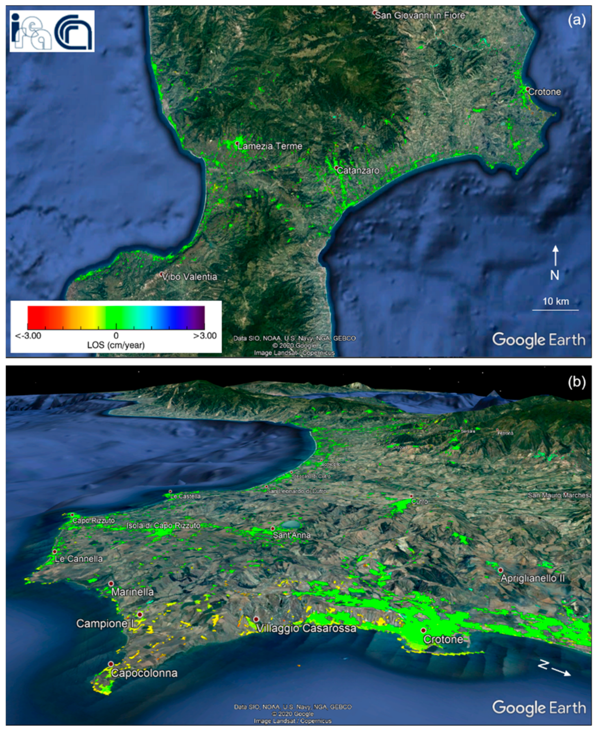
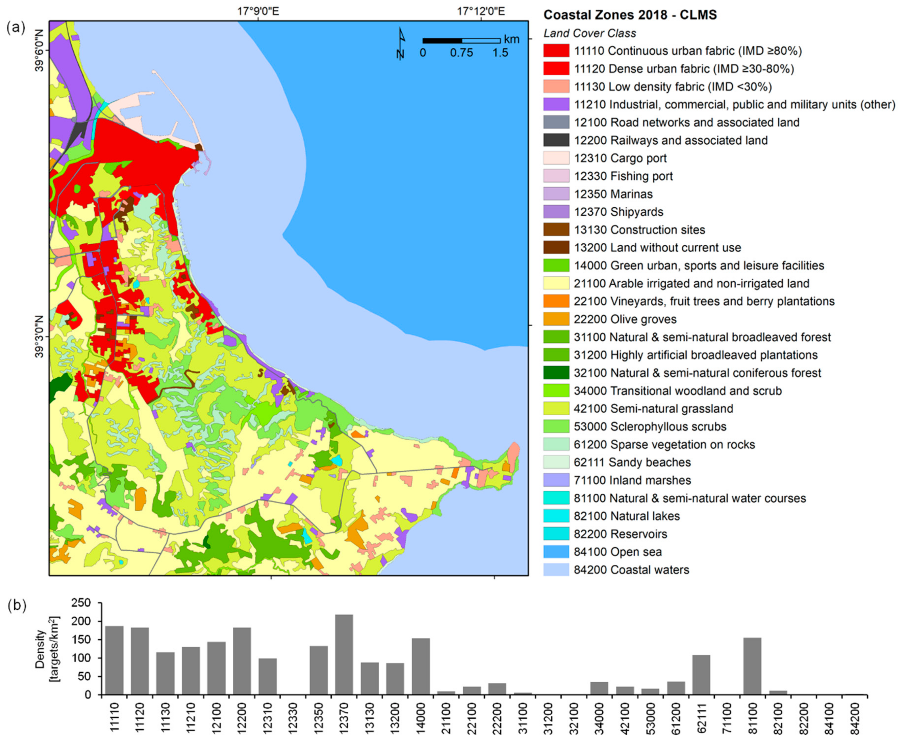
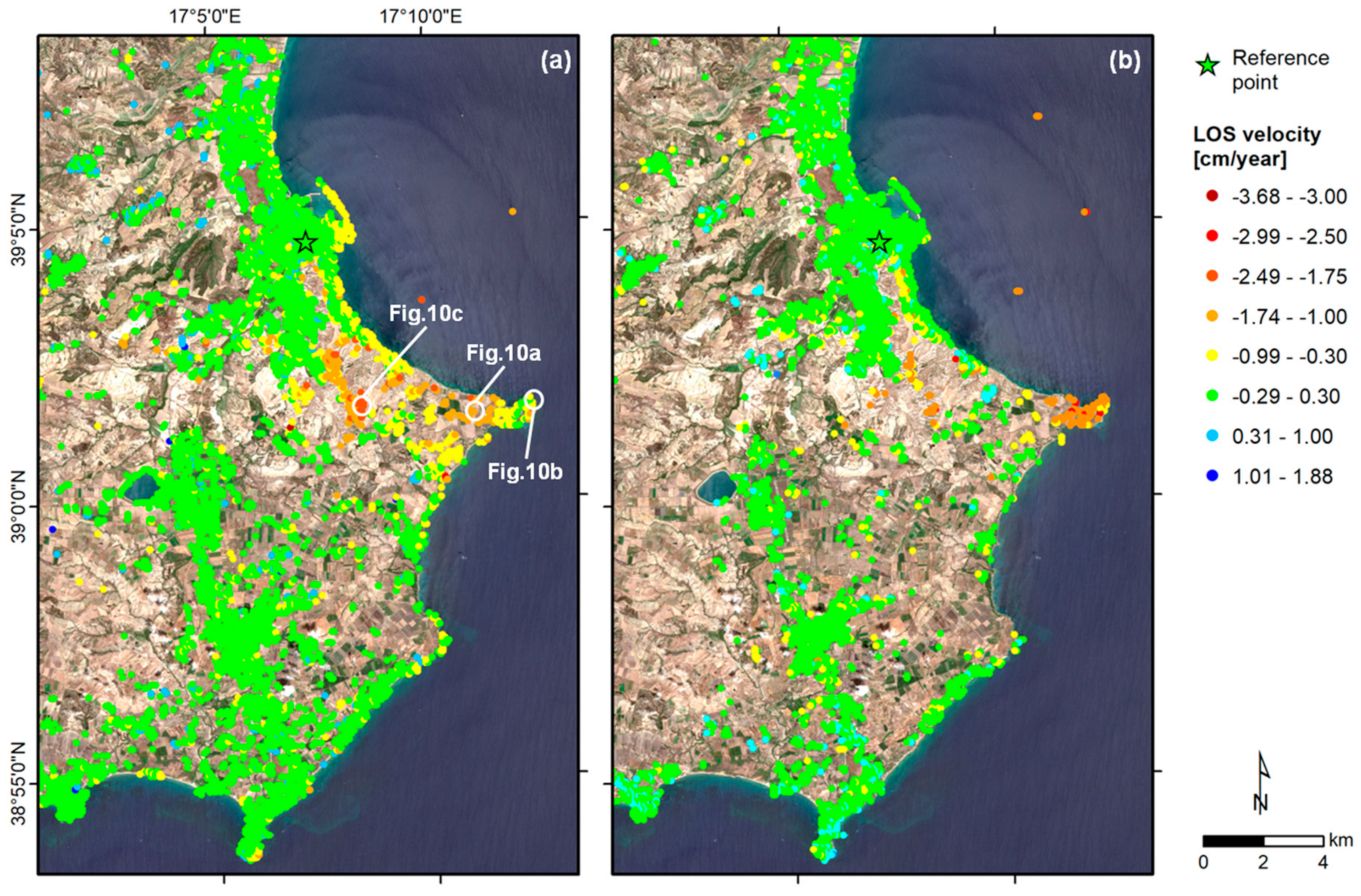
In hilly and mountains sectors of the study area that could be affected by mass movements, a simplified geomorphologic scheme was also considered (e.g., [83]), based on which deformation is more likely to occur along the steepest slope direction. This is true for translational slides, while it may not be suitable for the whole body of rotational landslides, topples and other types of mass movements, including erosion and calanchi landforms such as those present in some sectors of the study area.

Under the assumption that displacements occur along the steepest slope direction, the LOS estimates were projected onto it by considering the local values of terrain slope (β) and aspect (γ) as estimated from the SRTM DSM. These were used to identify the orientation of the steepest slope and its directional cosines at each location i, i.e., E_Si = sinγ_i*cosβ_i, N_Si = cosγ_i*cosβ_i, and U_Si = −sinβ_i.

The velocity along such direction (V_S) was then estimated as follows (e.g., [84]):

$$V_{Si} =\frac{V_{LOSi}}{E_{LOSi}\ast E_{Si}+N_{LOSi}\ast N_{Si}+U_{LOSi}\ast U_{Si}}$$

(3)

4. Results

The P-SBAS jobs for the whole processing area lasted 2.5 and 2.9 days for the Sentinel-1 IW ascending and descending datasets displayed in Figure 3, respectively. Therefore, these were the total times to process the stacks at full frame scale. In this particular experiment, two sub-swaths were processed for each geometry, given that the third covered only open waters (see Figure 3). The duration also includes the time required for sourcing the Sentinel-1 images to input into the processor from ESA’s repositories. Therefore, based on the above numbers, it can be well appreciated how advantageous and well-performing the P-SBAS parallel processing and GEP infrastructure were to ingest such high number of images, co-register, multi-look, build highly interconnected interferogram networks, and analyze them to extract thousands of coherent targets and their associated deformation time series.

Within the whole processed area (Figure 4), the retrieved number of targets using equal temporal coherence threshold of 0.85 was of 47,400 across 3800 km² land area for the ascending mode (~12.5 targets/km²), and 12,600 across 2000 km² for the descending mode (~6.3 targets/km²). The distribution and density of coherent targets reflected the land cover of the region (Figure 5), with vast expanses of forested areas of the Sila Massif, rural, and agricultural lands in the Crotone basin (where the step of phase-unwrapping was also more challenging), determining smaller densities of targets (e.g., 30–40 targets/km²; Figure 5b) with respect to densely covered urbanized sectors, coastal infrastructure and shipyards (e.g., 180–200 targets/km²), e.g., the city of Crotone (Figure 6). Coherent targets were also found at four offshore platforms (see Section 2; Figure 1b) thanks to their good coherence across the differential interferograms.

LOS velocity in 2014–2020 spanned between −3.7 and +1.6 cm/year in the ascending dataset, and between −2.0 and +1.9 cm/year in the descending dataset. Negative velocity values indicated movement away from the satellite sensor (yellow to dark red points in Figure 6a,b), while positive values indicated movement toward the sensor (light to dark blue points). Standard deviations with respect to a linear deformation model were 0.01 cm/year on average across the dataset of coherent targets, for both the ascending and descending mode. Maximum values of 0.09 and 0.05 cm/year were recorded for the ascending and descending datasets, respectively. The deformation histories were characterized by 0.3 cm standard errors on average across both datasets. These values provided an estimate of the precision of the P-SBAS datasets, and guided through the setting of the velocity range to identify coherent targets that could be considered stable (green points in Figure 6a,b). Standard errors for the time series were influenced by the presence of nonlinearities in the long-term deformation trend, as discussed in Section 5.

The vertical velocity field after combination of the two datasets showed widespread presence of negative velocities indicating subsidence, with observed rates as high as −4.7 cm/year. The largest subsiding zone was located at Capo Colonna promontory, where the rates reached −2.3 cm/year (Figure 7a). Along the Ionian coast and involving the harbor infrastructure another subsidence pattern can be recognized (Figure 8a). Within an active landslide area south of Crotone, the vertical rates also reached nearly −3.0 cm/year across a large sector (Figure 9).

The horizontal deformation field identified several sectors affected by eastward and westward displacement: (i) at the Capo Colonna archaeological site, where westward motion of up to −0.6 to −1.0 cm/year was recorded (Figure 7b); and (ii) across an elongated band involving the eastern coast between the Capo Colonna promontory and Crotone and including the old and new harbors of the city (Figure 8b), where eastward motion of +0.2 to +0.6 cm/year was found, with peaks reaching +1.0 cm/year.

5. Discussion

5.1. Geological Interpretation

The P-SBAS results highlight the presence of surface deformation processes that are related to known natural and anthropogenic hazards characterizing the study area (see Section 2): land subsidence in areas of gas extraction; landslides and erosion landforms; and subsidence due to settlement of modern infrastructure, intermingled with wider-scale motion patterns. It is worth noting that any long-wavelength deformation signals potentially affecting the study area are likely to have been subtracted from the datasets during the removal of residual orbital ramps (see Section 3.2), given that all long-wavelength signals (either deformation- or orbit-related) are typically treated as orbital errors, due to their similar spatial characteristics (e.g., [87]). This does not represent an issue for investigations of local scale processes, while it could impact studies of processes occurring across large scales (e.g., regional scale movements linked with tectonics), as their signals were suppressed during the above processing step.

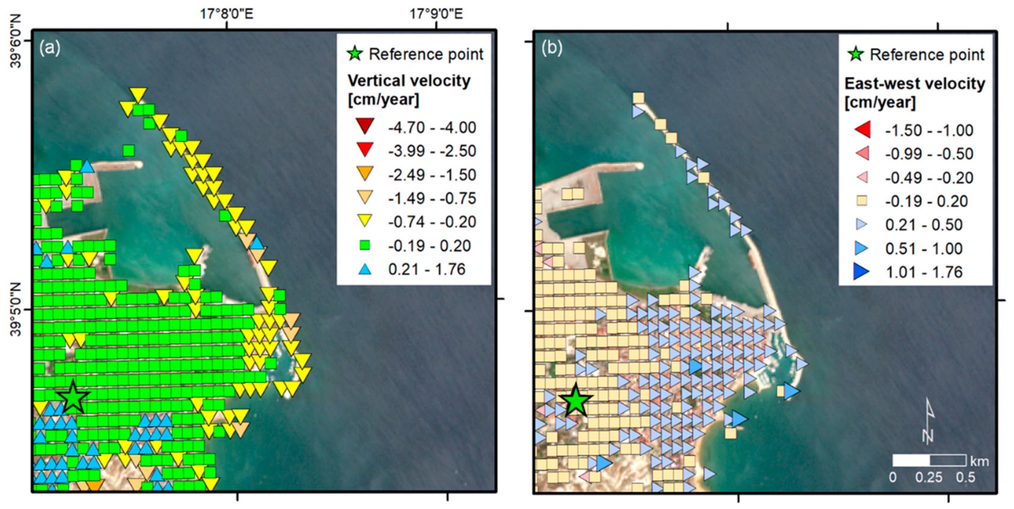
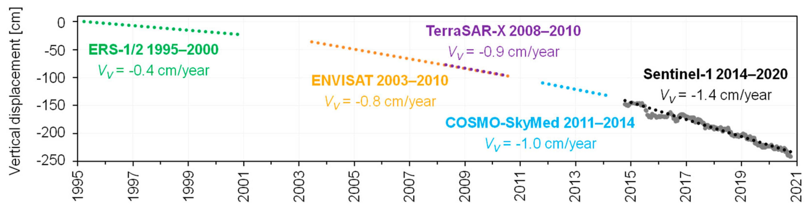
5.1.1. Coastal Land Subsidence at the Capo Colonna Promontory

The vertical and horizontal displacement field at Capo Colonna in 2014–2020 unequivocally highlights that the promontory is affected by land subsidence (Figure 7). The spatial configuration (albeit due to different causative factors) is, indeed, not dissimilar to other subsiding areas in Calabria region (e.g., Gioia Tauro [88]). V_U increases from inland and from the promontory coastline toward the central agricultural area, which is bounded by the spatial distribution of the gas wells (Figure 7a). The full displacement history for a coherent target at the center of the bowl is shown in Figure 10a through its LOS time series at the nearly 300 dates composing the dataset. Despite the lower density of coherent targets across the rural landscape, the east–west horizontal field makes evident that the motions converge toward this agricultural area, and this is the location around which the subsidence bowl appears to be centered (Figure 7b), i.e., west of the Hera Lacinia 001 production well. The evidence of such an east–west deformation field at the promontory is similar to earlier observations based on COSMO-SkyMed 2011–2014 data [28].

These results highlight a spatial association between land subsidence and gas extraction infrastructure that has been observed in previous studies. In this regard, in chronological order of publication,

Table 1. Existing InSAR literature covering the Capo Colonna promontory, with details on the input SAR data, monitoring period covered, and the observed deformation rates. Notation: asc. = ascending; desc. = descending.

Reference	Satellite Data	Period	Observed Deformation Rates
Basili et al. 2010 [38]	ERS-1/2 asc. ENVISAT asc.	1995–2000 2002–2009	More than −0.5 cm/year LOS rate
Tapete and Cigna 2012 [39]	ERS-1/2 asc./desc. ENVISAT asc.	1992–2000 2003–2010	Up to −1.0 (1992–2000) and −1.3 (2003–2010) cm/year LOS rate
Confuorto et al. 2016 [45]	TerraSAR-X asc./desc.	2008–2010	Up to −1.5 cm/year LOS rate, and −1.6 cm/year vertical rate
Cigna et al. 2016 [46]	ERS-1/2 asc./desc. (from [39]) ENVISAT asc. (from [39]) TerraSAR-X asc./desc. (from [45]) COSMO-SkyMed asc./desc. Sentinel-1A asc.	1992–2000 2003–2010 2008–2010 2011–2015 2014–2016	Up to −2.0 (2011–2014), −1.0 (2014–2015) and −0.8 (2014–2016) cm/year LOS rate; up to −20 cm vertical displacement (1992–2016; stitched time series)
Zecchin et al. 2018 [28]	COSMO-SkyMed asc./desc.	2011–2014	Up to −0.5 cm/year east–west rate
Cigna and Tapete 2020 1	Sentinel-1A/B asc./desc.	2014–2020	Up to −2.3 cm/year vertical and −1.0 cm/year east–west rate

¹ This article.

summarizes journal papers, proceedings, and technical reports that include InSAR analyses of land subsidence at Capo Colonna. Of these, the majority focused on InSAR datasets retrieved from one to two SAR sensor datasets. Whereas [46] provided not only the most recent assessment using COSMO-SkyMed ascending and descending (2011–2015) and Sentinel-1A ascending (2014–2016) data, but also a 25-year-long review of local land subsidence through the combination with other C- and X-band InSAR datasets from 1992 to 2010.

Up to −2.0 (2011–2014), −1.0 (2014–2015) and −0.8 (2014–2016) cm/year LOS rate; up to −20 cm vertical displacement (1992–2016; stitched time series)

Comparison of the Sentinel-1 P-SBAS outputs with past observations available in the literature allowed corroboration of the spatial patterns and the order of magnitude of the deformation rates affecting the study area. In particular, the present results corroborate the spatial patterns of land subsidence that were found with ERS-1/2 ascending and descending data processed with SBAS [38] and Permanent Scatterers InSAR (PS-InSAR) [39,46], ENVISAT ascending data with SBAS [38] and Persistent Scatterers Pairs–DIFferential InSAR (PSP–DIFSAR) [39,46], TerraSAR-X ascending and descending data with SBAS [45,46], and COSMO-SkyMed ascending and descending data with PSP-DIFSAR and the Coherent Pixel Technique–Temporal Sublook Coherence (CPT–TSC) [46]. It is worth noting that a quantitative comparison of 2014–2020 deformation rates with those observed in these past studies is not viable due to their different time coverage.

Such corroboration is achieved through a significant improvement in terms of both InSAR processing and post-processing of coherent targets and their time series. In particular, most of the previous studies on Capo Colonna relied on LOS displacement values only [38,39,46] and, when the authors of those papers attempted the extraction of deformation components, they limited it to either the vertical [45,46] or east–west [28] deformation field. Therefore, the present study is the first that, at least for the last six years, is able to fully constrain the geometry of the land subsidence process at the promontory not only along the LOS, but also along both the vertical and east–west directions.

Furthermore, a closer look at the temporally dense InSAR time series highlights that the displacement trend of land subsidence has been almost constant over the study period (Figure 10a), with a magnitude of total displacement that makes a clear separation between the subsiding points and the more stable ones (Figure 10b). Pending an in-depth time series analysis (also through statistical methods, which is beyond the scope of this research), the nonlinearities visible throughout the time series do not seem to coincide with any significant deceleration or inversion of the land subsidence trend. Future research will also need to focus on the temporally confined trend variations occurred in July–October 2016 and September–October 2018, which will have to be further investigated through comparison with independent in situ monitoring data (not available for this research).

In this regard, the present analysis allows a revisit of the assessment made based on an earlier Sentinel-1 dataset, in which a slight decrease in the annual LOS velocities of subsidence around the gas extraction sites was suggested [46]. That dataset consisted of 46 ascending mode images only, collected by the Sentinel-1A satellite alone, every 12 days, from October 2014 to May 2016, and was processed with an intermittent SBAS [89] processing method capable of extending the coverage of motion results across the full range of land-cover types by relaxing the approach to selecting image pixels to process [90]. Therefore, despite the high density of coherent pixels over the agricultural area provided in [46], the limited length of the image datasets somehow might have affected the estimation of the deformation velocity by tying it to a shorter time period. On the other hand, with nearly 300 displacement estimates composing the InSAR time series in each Sentinel-1 observation geometry (Figure 11), the current P-SBAS analysis provides a more robust evidence of the uninterrupted land subsidence long-term behavior and its rate of occurrence.

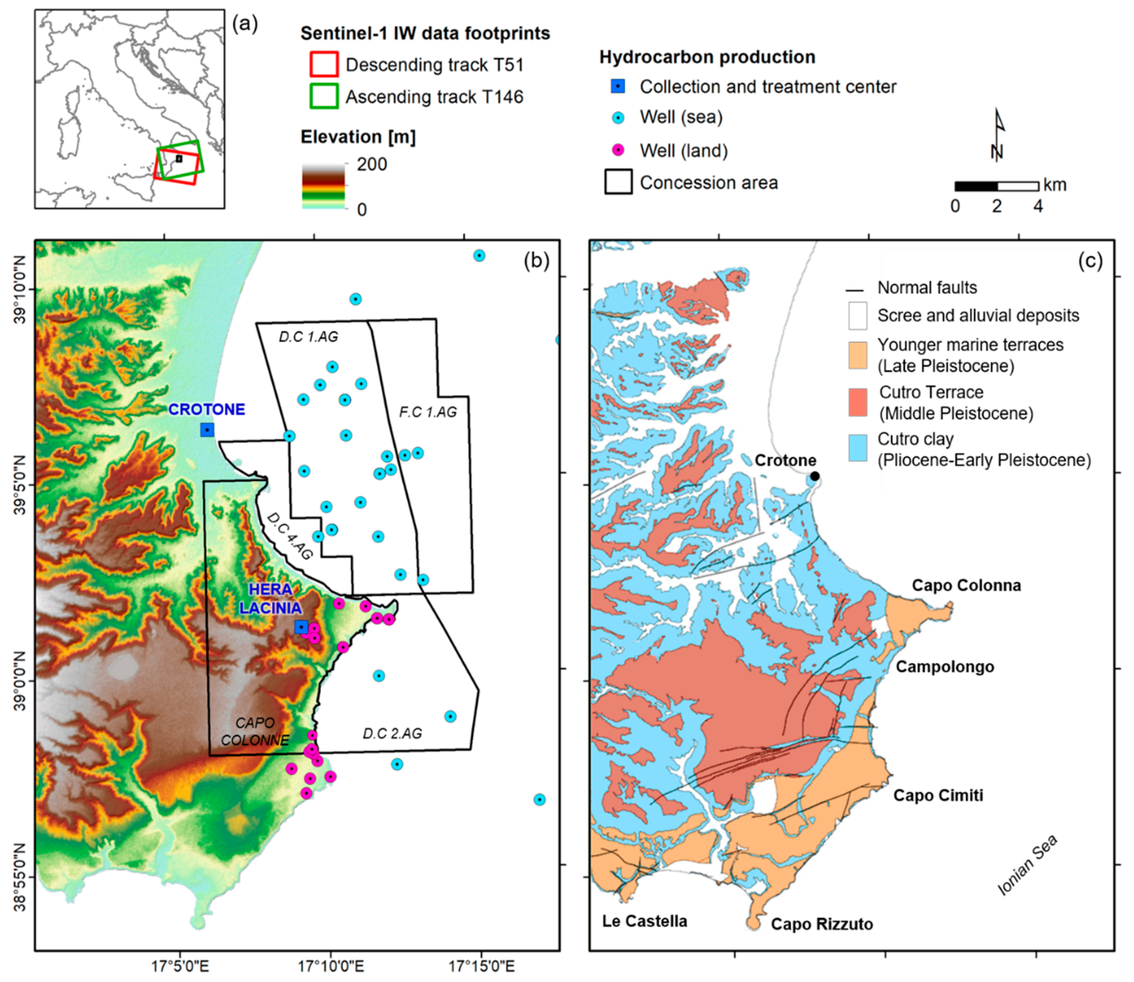
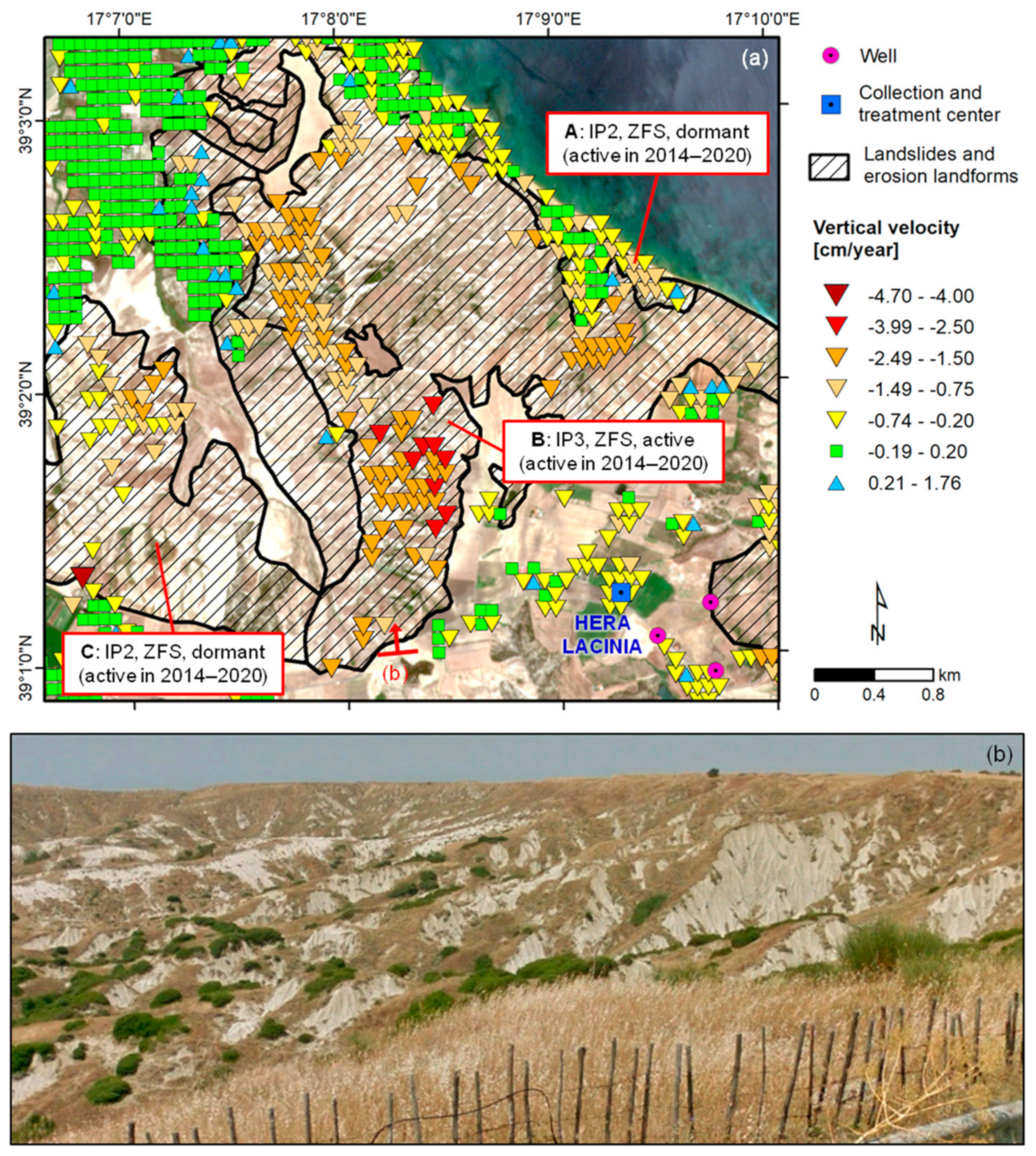
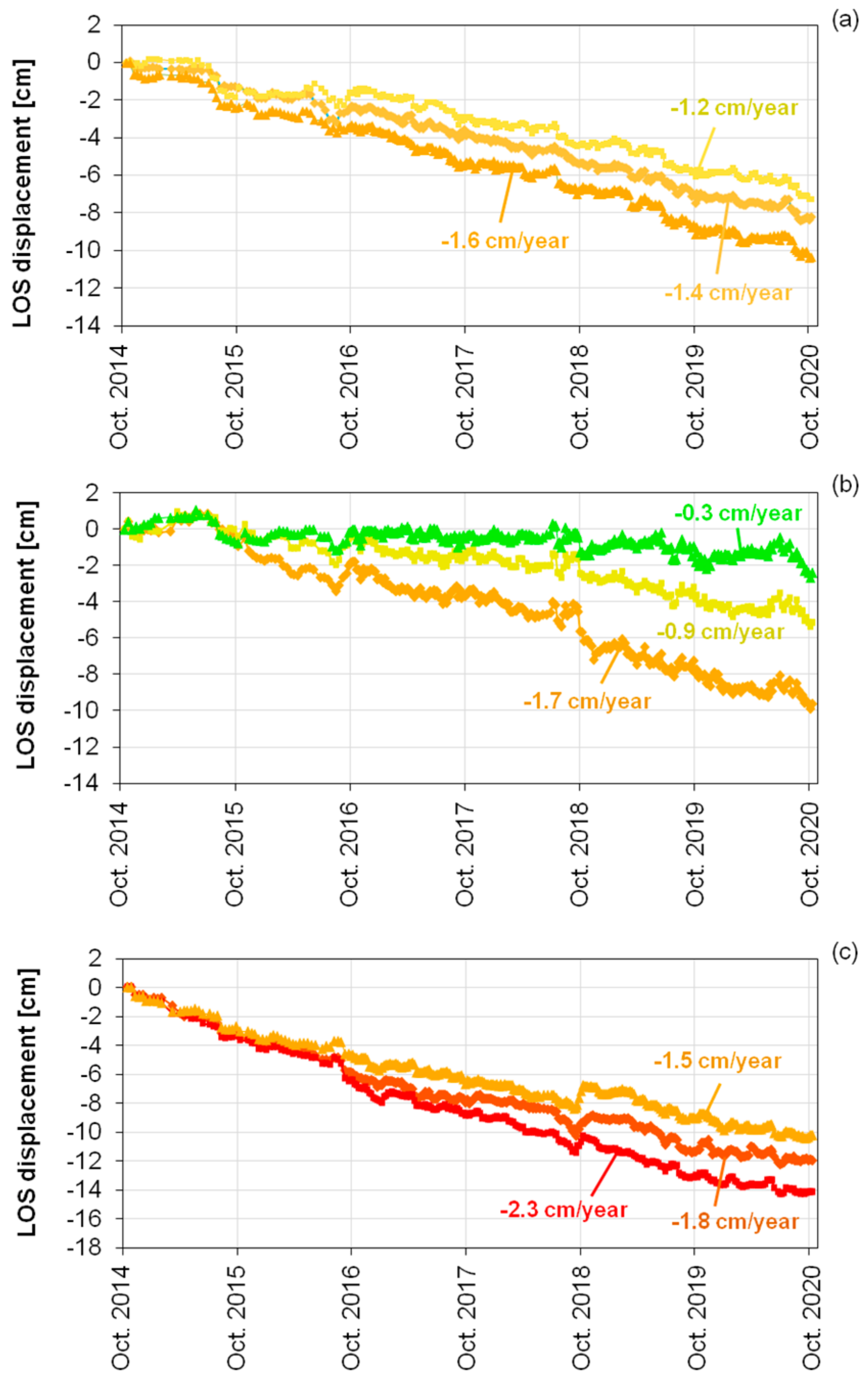
5.1.2. Landslides and Erosion Landforms

South of the city of Crotone and northwest of the Capo Colonna promontory, the V_U map highlights two elongated patterns and a more circular one of vertical motions (Figure 9a) that cannot be attributed to land subsidence, given their shape and underlying topography, but instead to mass movement processes. As both ascending and descending mode data were exploited in the analysis, the directional variety of mass movements in this zone was taken into account. In turn, both east-facing and west-facing slopes were visible to the Sentinel-1 LOS and covered with targets from at least one P-SBAS output dataset.

The first pattern of vertical motions, generally up to −0.75 cm/year with a few peaks of −1.0 to −1.4 cm/year, covers the narrow coastline section where, according to the Hydrogeological Setting Plan (Piano Stralcio per l′Assetto Idrogeologico, PAI) updated in 2016 by the River Basin Authority of Calabria Region [86], a dormant landslide area with a medium hazard level (i.e., hazard index IP2) is mapped (i.e., polygon A in Figure 9a). Within the boundary of this polygon, the velocity along the steepest slope direction is generally lower than 5 cm/year, with some peaks at 30–50 cm/year. As per the simplified geology reported in Figure 1c [30], the bedrock lithology is made of Pliocene–Early Pleistocene clays, which are known for their susceptibility to local slope-wash processes, particularly in non-vegetated areas (Figure 2; [49]; see Section 2). According to the Copernicus Land Monitoring Service Coastal Zones dataset (Figure 5a; [85]), the land cover at the slope foot is mainly “industrial, commercial, public and military units (other)”, “continuous urban fabric”, and “construction sites”. These classes match with the Google Earth satellite observation of residential buildings, leisure estates, and local commercial activities distributed along the SP49 road connecting Crotone with the Capo Colonna promontory and the southern part of the province.

The second elongated pattern of vertical motions, up to nearly −3.0 cm/year, is located on top of a superficial landslide zone (i.e., polygon B in Figure 9a) classified in PAI 2016 [86] as active with a high hazard level (i.e., hazard index IP3), and where calanchi landforms (Figure 9b) have been recognized [49]. The velocity along the steepest slope direction reaches 10–50 cm/year at several locations within the mapped landslide zone, though in this case this may not be the predominant deformation direction for the whole landslide body, given the existence of some accumulation zones, as well as some scarps. Displacement time series for the coherent targets within this zone show a clear trend reaching up to −15 cm of total LOS displacement in the observation period (Figure 10c). More to the west, a third cluster of coherent targets moving vertically up to −2.4 cm/year defines a nearly circular pattern indicating deformation at another calanchi landform (i.e., polygon C in Figure 9a) [49] that is classified in the PAI 2016 [86] as a dormant superficial landslide zone with a medium hazard level (IP2). Velocity values along the steepest slope direction are lower than 5 cm/year across most of the feature. Both the landslide areas exhibit a rural land cover ranging from sparse vegetation to scrubland and grassland (Figure 5a).

Since the P-SBAS results provide more recent information than the data used for the PAI 2016 classification, the above velocity values suggest the opportunity to update the state of activity of these landslide and calanchi landforms, by applying the PSI-based matrix approach [84,91] that was originally tested in northern and central Calabria. By referring to the displacement rates observed in 2014–2020 at each mass movement area, it turns out that, while the active state of the IP3 landslide body (polygon B in Figure 9a) is confirmed and the intensity of the process belongs to the category of very slow processes (i.e., velocity of 16 mm/year to 1.6 m/year; according to [92]), the hazard classification of the IP2 landslide bodies (polygons A and C in Figure 9a) should be revised from dormant to active with extremely slow (i.e., velocity less than 16 mm/year) and very slow intensity, respectively, if considering their vertical rates (while estimates along the steepest slope direction suggest that both processes occur with very slow intensity). On the other side, given that most of these landslide bodies are calanchi, the proposed reclassification based on the found motions has to be interpreted in the context of the typical behavior of these landforms, which are characterized by washing and weathering processes, and conditioned by local rainfall regime.

Future in-depth analysis of these processes could also account for local precipitation records to investigate any potential correlation with the deformation observed in the satellite results and highlight impacts on landslide triggering and/or reactivation.

5.1.3. Ground Deformation in the City of Crotone

Across the whole P-SBAS datasets, the other zone with negative LOS velocity values that can be clearly detected is located over the harbors of the city of Crotone (Figure 6). In particular, this pattern comes out very distinctively even with the naked eye in the ascending geometry dataset (Figure 6a), where LOS velocity is estimated at up to −1 cm/year. The rest of the city instead appears overall stable in both geometries, as expected for an historic urban settlement (Figure 6a,b). However, this evidence links with the reference point that was set within the urban area (see green star in Figure 6), and so any deformation signal is relative to such point.

By analyzing the P-SBAS data in more detail, and specifically the vertical displacement field (Figure 8a), coherent targets with V_U values reaching −0.75 to −1.3 cm/year are distributed along the 1.7 km-long breakwater of the new harbor, as well as along the smaller breakwater and over the commercial and residential buildings overlooking the old harbor. A reasonable explanation of such subsidence might be the typical settlement of the harbor infrastructure, also as a consequence of recent interventions and maintenance works. In this regard, it is worth recalling that LOS displacement rates between −0.2 and −0.5 cm/year had been already found with ERS-1/2 and ENVISAT data in the period 1995–2009 [38].

The horizontal field (Figure 8b) provides a further interesting insight, given that both the breakwaters and most of the old town (including the massive Castle of Charles V) fall within a wide pattern of eastward deformation, with V_E ranging between +0.2 and +0.6 cm/year. Such pattern corroborates the evidence of +0.3 to +0.5 cm/year found with COSMO-SkyMed data for the period 2011–2014 [28]. Any slight difference between the two InSAR analyses could mainly be due to the different time periods surveyed, as well as the different techniques used to process the SAR data and the respective processing parameters that were set up, above all the reference point and its precise location within a known tectonically active region. Continuous geodetic monitoring data from two GPS stations installed in Crotone (CROT and KROT) indeed confirmed the presence of significant eastward horizontal motions, alongside northward ones [93]. The latter, however, are not captured in the P-SBAS results due to the known relatively poor visibility of north–south horizontal movements to the SAR sensor LOS, and the V_N=0 assumption that was made to estimate the vertical and east–west deformation field (see Section 3.3). In this case, such an assumption prevents any north–south displacement to be estimated, and also introduces an error in the other two components (vertical and east–west), especially at locations where a significant north–south displacement occurs [81]. Detailed date-by-date comparison of the P-SBAS and GPS monitoring data at the two stations would require the setting of a local reference frame for the GPS stations and the calibration of the P-SBAS results to the same reference system, as done in [28]. This would enable the quantification of the P-SBAS datasets accuracy against external data, though such analysis is beyond the scientific goals of this study.

5.2. Potential and Challenges of Big Data

The above results and geological interpretation demonstrate how the paradigm of InSAR studies is rapidly changing not only with the advent of SAR big data, but also owing to the accessibility of cloud/grid infrastructure and chains to process such huge datasets.

The nearly 300 images per single observation geometry that were processed to cover the study area of this paper well represent the typical big SAR stack that a satellite constellation such as Sentinel-1 is already able to provide, now that its two twin satellites have been collecting images globally for more than six years, with a site revisit of up to six days. Even if the site revisit was constrained to 12 days only (as it currently is in geographic areas outside Europe; [9]), the constellation would still collect 30 images per year. To put this number into context, this exceeds the typical minimum amount of C-band SAR images per single observation geometry that InSAR practitioners consider as the minimum requirement to carry out a meaningful and reliable PSI processing (i.e., 15–20 scenes; [5]), regardless of the total period of observation. The latter plays a crucial role. Relatively short time periods might be unable to capture the long-term behavior of the deformation processes of interest, and/or be biased by the occurrence of annual fluctuations or other short-term dynamics that could influence the estimation of deformation rates. Therefore, the use of Sentinel-1 imagery to investigate “silent” and subtly evolving geohazards that manifest over long periods and with trends that can be captured over years (such as the slow-moving landslides and coastal subsidence investigated in the province of Crotone), today poses the technical challenge of processing big SAR stacks with adequate computing resources.

Our experiment proves that nowadays, with the GEP it is possible to process a whole time series of 300 Sentinel-1 SAR images at full swath in less than three days, without the necessity for in-house high-performance computers and data-storage capacity (as an approximate figure with which to compare this time performance, the same processing in a standard desktop PC could take over a week or more, depending on its hardware configuration). The latter aspect is frequently overlooked when planning an InSAR investigation, but it should not be. A stack of 300 SLC Sentinel-1 dual-polarization images alone, prior to any pre-processing or InSAR analysis, requires approximately 2.4 terabytes of disk space, not to mention that these input data need to be sourced from a repository, and this step normally requires a certain amount of time given the conditions for data downloading from catalogues (e.g., a maximum of two simultaneous image downloads as currently allowed to users by the Copernicus Open Access Hub). On the other hand, it is reasonable to expect that a more direct connection to the data repository and a faster data retrieval, combined with a greater amount of computing resources made available to run the processing steps, can significantly improve the overall performance with total processing times shorter than the ~3 days achieved in this experiment. Other P-SBAS studies carried out over the same and larger regions of interest across Italy [54,59] report processing time demands of less than one day, though they refer to shorter Sentinel-1 stacks (i.e., ~120–180) and a different cloud-computing infrastructure (i.e., AWS). Therefore, a one-to-one quantitative comparison of time demands cannot be made against these studies.

Nonetheless, there is no doubt that a processing run in the GEP saves time that can instead be invested by users to tailor the processing parameters, post-process and interpret the output InSAR products to address their scientific and/or technical goals (e.g., creating a hazard map, estimating landslide intensity, modeling the subsidence process). In this regard, in the GEP, the selection of parameters such as the number and acquisition date of the input SAR data, the study area (clip to AOI), the processing thresholds (e.g., temporal coherence), and the location of the reference point, is allowed through the geo-portal within the framework of a consolidated and standardized P-SBAS processing routine. In the case of Capo Colonna and Crotone, this functionality has definitely been advantageous compared to previous studies that exploited already processed and ready-to-use InSAR datasets [28,39,46]. At equal opportunity of reliance on trustable InSAR datasets produced by means of consolidated processing routines, in the present experiment, we could tailor the processing parameters to suit our purposes (e.g., reference point selection and respective implications, as discussed in Section 5.1.3).

On the other side, compared to those papers investigating land subsidence and regional tectonics in the study area based on InSAR products generated by the authors themselves [38,45,46], the processing times achieved thanks to the use of the GEP were extremely short on a relative scale, especially when considering that the Sentinel-1 stacks used in the present study were one order of magnitude longer (i.e., 300 vs. 40–60 images). A drawback is, of course, due to the current limitations in the range of SAR sensors that can be selected for P-SBAS processing in the GEP. At present, the P-SBAS on-demand service runs with Sentinel-1 data only, and it is also available for ERS-1/2 and ENVISAT SAR data archives via a link with the ESA G-POD platform [55].

Of course, such eased accessibility to reliable InSAR products does not solve the challenge of how to manage the post-processing and geospatial analysis of hundreds of thousands (or even millions) of coherent points. In the present research, given the intended demonstration character of this paper and the regional scale of the geohazard analysis (therefore, with no intention to deepen the geological interpretation beyond the correlation between the observed motions and the type of natural and/or anthropogenic process), the multitude of coherent points was creamed-off by narrowing down the geological interpretation to a relatively small region of 300 km², and to its most relevant displacement patterns. This was done based on the initial LOS velocity values and the extracted vertical and horizontal displacement field, and then through geospatial integration with ancillary data (e.g., lithological map, landslide inventory) and the literature (e.g., evidence from previous InSAR studies). Such an approach is viable and effective when there is strong background knowledge of the geohazards affecting the study area. In other contexts, methods such as hotspot identification and clustering [94], time series analysis and estimation of trend deviations [15,17,95], statistical tests, and probabilistic approaches [16,17,18] are recommended.

Research trends in the field of InSAR are now aiming toward the development of processing chains and approaches to continuously update multi-interferogram processing outputs (as well as their post-processing and automated analysis) every time that one or more new SAR scenes are available for the study area. These approaches may provide key information for monitoring and early warning of the occurrence of anomalous trends and/or acceleration associated with precursors or incipient deformation processes, and thus input alerting and operational monitoring services (e.g., [25,96]). To achieve these goals, efficient approaches for data reprocessing after new data inputs become available are required to optimize processing loads and times (in the order of a few hours; [25]) for the updating of a multi-interferogram processing (e.g., via a sequential estimator; [97]). Currently, the P-SBAS service available in ESA’s GEP does not include such functionality, and therefore the benefit of these approaches on its time performance cannot be assessed in this case.

6. Conclusions

In this study, six full years of Sentinel-1 SAR ascending and descending mode imagery were processed with the P-SBAS service available in ESA’s GEP to generate the longest ever interferometric stacks so far used for a single study site and published in the specialist SAR remote sensing literature. The multitude of coherent points retrieved and the respective LOS displacement time series were then analyzed to develop use-cases of geological interpretation related to “silent” and subtle hazards—i.e., slow-moving landslides, erosion landforms, and coastal subsidence—affecting different locations spread across the province of Crotone in Calabria, southern Italy.

The results achieved make this research novel because they demonstrate that Sentinel-1 time series in the order of nearly 300 images (per observation geometry) can be processed in less than three days, owing to the high-performance computing infrastructure available in the GEP. Tens of thousands of coherent points can therefore be retrieved through P-SBAS, with a level of spatial density that is suitable to depict deformation patterns in rural and agricultural land-cover types as well. Furthermore, the very frequent displacement time series provided for each coherent point enable a robust identification of not only the long-term deformation trend of natural and anthropogenic hazard processes, but also of their short-term variations on a weekly basis, which previous analyses relying on shorter data stacks (or long stacks with less frequent observations) for the same study area could struggle to unveil. This comes out evidently in the characterization of the temporal evolution of land subsidence at the Capo Colonna promontory. Any investigations of shorter time spans, indeed, could be biased by the occurrence of seasonal or intra-annual variations, and therefore would not be able to provide a robust estimate of the long-term trend. On the other hand, long time spans with less frequent observations (e.g., on the monthly or bimonthly scale) may not be able to sense shorter scale non-linearities. Therefore, the geo-information provided by the 300 image-long datasets with weekly revisit acts as a key input for investigations of geological processes.

In this regard, the choice of a study area that was previously investigated with InSAR techniques proved effective to highlight the advantages brought by P-SBAS processing of such big SAR data, and thus helped to demonstrate the concept of how to develop applications with such big InSAR products for geohazard assessment and environmental monitoring purposes. Post-processing of P-SBAS results according to well-established methods included the vertical and east–west deformation field estimation, and the PSI-based matrix approach for landslide activity assessment.

In the case of Capo Colonna, the vertical and east–west deformation field estimation allowed constraining of the geometry of land subsidence and locating the center of the subsidence bowl, thus confirming and bringing in new knowledge compared to previous InSAR observations that were limited to analysis of LOS displacements, or only one of the two deformation components. In Crotone, the method helped to discriminate different sectors of the city (harbors, old town, inland settlement) and to detect horizontal motions that relate to the regional tectonics.

Finally, the exercise of updating the existing landslide inventory by means of the PSI-based matrix approach was intentionally meant as a simple, but effective proof-of-concept of the types of value-adding that users can undertake if they have access to the platform and become familiar with generating and exporting P-SBAS products to input them into their workflows for the generation of thematic products and development of downstream applications.

References

1. Gabriel, A.K.; Goldstein, R.M.; Zebker, H.A. Mapping small elevation changes over large areas: Differential radar interferometry. J. Geophys. Res. 1989, 94, 9183–9191. [Google Scholar] [CrossRef]
2. Massonnet, D.; Feigl, K.L. Radar interferometry and its application to changes in the earth’s surface. Rev. Geophys. 1998, 36, 441–500. [Google Scholar] [CrossRef] [Green Version]
3. Rosen, P.A.; Hensley, S.; Joughin, I.R.; Li, F.K.; Madsen, S.N.; Rodriguez, E.; Goldstein, R.M. Synthetic aperture radar interferometry. Proc. IEEE 2000, 88, 333–380. [Google Scholar] [CrossRef]
4. Ferretti, A.; Prati, C.; Rocca, F. Permanent scatterers in SAR interferometry. IEEE Trans. Geosci. Remote Sens. 2001, 39, 8–20. [Google Scholar] [CrossRef]
5. Crosetto, M.; Monserrat, O.; Cuevas-González, M.; Devanthéry, N.; Crippa, B. Persistent Scatterer Interferometry: A review. ISPRS J. Photogramm. Remote Sens. 2016, 115, 78–89. [Google Scholar] [CrossRef] [Green Version]
6. Berardino, P.; Fornaro, G.; Lanari, R.; Sansosti, E. A new algorithm for surface deformation monitoring based on small baseline differential SAR interferograms. IEEE Trans. Geosci. Remote Sens. 2002, 40, 2375–2383. [Google Scholar] [CrossRef] [Green Version]
7. Lanari, R.; Mora, O.; Manunta, M.; Mallorquí, J.J.; Berardino, P.; Sansosti, E. A small-baseline approach for investigating deformations on full-resolution differential SAR interferograms. IEEE Trans. Geosci. Remote Sens. 2004, 42, 1377–1386. [Google Scholar] [CrossRef]
8. Virelli, M.; Coletta, A.; Battagliere, M.L. ASI COSMO-SkyMed: Mission Overview and Data Exploitation. IEEE Geosci. Remote Sens. Mag. 2014, 2, 64–66. [Google Scholar] [CrossRef]
9. ESA Sentinel-1 Observation Scenario. Available online: https://sentinel.esa.int/web/sentinel/missions/sentinel-1/observation-scenario (accessed on 26 March 2020).
10. Gomes, V.C.F.; Queiroz, G.R.; Ferreira, K.R. An overview of platforms for big Earth observation data management and analysis. Remote Sens. 2020, 12, 1253. [Google Scholar] [CrossRef] [Green Version]
11. Sudmanns, M.; Tiede, D.; Lang, S.; Bergstedt, H.; Trost, G.; Augustin, H.; Baraldi, A.; Blaschke, T. Big Earth data: Disruptive changes in Earth observation data management and analysis? Int. J. Digit. Earth 2020, 13, 832–850. [Google Scholar] [CrossRef]
12. ESA Copernicus Open Access Hub. Available online: https://scihub.copernicus.eu/dhus (accessed on 1 November 2020).
13. Zinno, I.; Casu, F.; De Luca, C.; Elefante, S.; Lanari, R.; Manunta, M. A Cloud Computing Solution for the Efficient Implementation of the P-SBAS DInSAR Approach. IEEE J. Sel. Top. Appl. Earth Obs. Remote Sens. 2017, 10, 802–817. [Google Scholar] [CrossRef]
14. Loibl, D.; Bookhagen, B.; Valade, S.; Schneider, C. OSARIS, the “open source SAR investigation system” for automatized parallel insar processing of Sentinel-1 time series data with special emphasis on cryosphere applications. Front. Earth Sci. 2019, 7, 172. [Google Scholar] [CrossRef] [Green Version]
15. Cigna, F.; Tapete, D.; Casagli, N. Semi-automated extraction of Deviation Indexes (DI) from satellite Persistent Scatterers time series: Tests on sedimentary volcanism and tectonically-induced motions. Nonlinear Process. Geophys. 2012, 19, 643–655. [Google Scholar] [CrossRef] [Green Version]
16. Berti, M.; Corsini, A.; Franceschini, S.; Iannacone, J.P. Automated classification of Persistent Scatterers Interferometry time series. Nat. Hazards Earth Syst. Sci. 2013, 13, 1945–1958. [Google Scholar] [CrossRef] [Green Version]
17. Notti, D.; Calò, F.; Cigna, F.; Manunta, M.; Herrera, G.; Berti, M.; Meisina, C.; Tapete, D.; Zucca, F. A User-Oriented Methodology for DInSAR Time Series Analysis and Interpretation: Landslides and Subsidence Case Studies. Pure Appl. Geophys. 2015, 172, 3081–3105. [Google Scholar] [CrossRef] [Green Version]
18. Chang, L.; Hanssen, R.F. A Probabilistic Approach for InSAR Time-Series Postprocessing. IEEE Trans. Geosci. Remote Sens. 2016, 54, 421–430. [Google Scholar] [CrossRef] [Green Version]
19. Casu, F.; Elefante, S.; Imperatore, P.; Zinno, I.; Manunta, M.; De Luca, C.; Lanari, R. SBAS-DInSAR Parallel Processing for Deformation Time-Series Computation. IEEE J. Sel. Top. Appl. Earth Obs. Remote Sens. 2014, 7, 3285–3296. [Google Scholar] [CrossRef]
20. Foumelis, M.; Papadopoulou, T.; Bally, P.; Pacini, F.; Provost, F.; Patruno, J. Monitoring Geohazards Using On-Demand and Systematic Services on ESA’s Geohazards Exploitation Platform. In Proceedings of the International Geoscience and Remote Sensing Symposium (IGARSS), Yokohama, Japan, 28 July–2 August 2019; IEEE: Yokohama, Japan, 2019; pp. 5457–5460. [Google Scholar]
21. Committee on Earth Observation Satellites (CEOS). CEOS WG Disasters: Working Group on Disasters. Available online: http://ceos.org/ourwork/workinggroups/disasters/ (accessed on 3 November 2020).
22. Lanari, R.; Bonano, M.; Casu, F.; De Luca, C.; Manunta, M.; Manzo, M.; Onorato, G.; Zinno, I. Automatic Generation of Sentinel-1 Continental Scale DInSAR Deformation Time Series through an Extended P-SBAS Processing Pipeline in a Cloud Computing Environment. Remote Sens. 2020, 12, 2961. [Google Scholar] [CrossRef]
23. Burnol, A.; Foumelis, M.; Gourdier, S.; Deparis, J.; Raucoules, D. Tracking and measuring of clay shrinking and swelling using spaceborne remote sensing. EarthArxiv 2020. [Google Scholar] [CrossRef]
24. Cigna, F.; Tapete, D. Present-day land subsidence rates, surface faulting hazard and risk in Mexico City with 2014–2020 Sentinel-1 IW InSAR. Remote Sens. Environ. 2021, 253, 1–19. [Google Scholar] [CrossRef]
25. Bakon, M.; Czikhardt, R.; Papco, J.; Barlak, J.; Rovnak, M.; Adamisin, P.; Perissin, D. remotIO: A Sentinel-1 Multi-Temporal InSAR Infrastructure Monitoring Service with Automatic Updates and Data Mining Capabilities. Remote Sens. 2020, 12, 1892. [Google Scholar] [CrossRef]
26. Guerricchio, A. Tectonics, Deep Seated Gravitational Slope Deformations (DSGSDs) and Large Landslides in the Calabrian Region (Southern Italy). G. Geol. Appl. 2005, 1, 73–90. [Google Scholar] [CrossRef]
27. Stanley, J.D.; Bernasconi, M.P. Buried and submerged greek archaeological coastal structures and artifacts as gauges to measure late holocene seafloor subsidence off Calabria, Italy. Geoarchaeology 2012, 27, 189–205. [Google Scholar] [CrossRef]
28. Zecchin, M.; Accaino, F.; Ceramicola, S.; Civile, D.; Critelli, S.; Da Lio, C.; Mangano, G.; Prosser, G.; Teatini, P.; Tosi, L. The Crotone Megalandslide, southern Italy: Architecture, timing and tectonic control. Sci. Rep. 2018, 8, 1–11. [Google Scholar] [CrossRef] [PubMed]
29. Ministero dello Sviluppo Economico, MISE. MISE Ricerca e Coltivazione di Idrocarburi. Available online: https://unmig.mise.gov.it/index.php/it/dati/ricerca-e-coltivazione-di-idrocarburi (accessed on 30 September 2020).
30. Zecchin, M.; Civile, D.; Caffau, M.; Sturiale, G.; Roda, C. Sequence stratigraphy in the context of rapid regional uplift and high-amplitude glacio-eustatic changes: The Pleistocene Cutro Terrace (Calabria, southern Italy). Sedimentology 2011, 58, 442–477. [Google Scholar] [CrossRef]
31. Zecchin, M.; Civile, D.; Caffau, M.; Roda, C. Facies and cycle architecture of a Pleistocene marine terrace (Crotone, southern Italy): A sedimentary response to late Quaternary, high-frequency glacio-eustatic changes. Sediment. Geol. 2009, 216, 138–157. [Google Scholar] [CrossRef]
32. Minelli, L.; Billi, A.; Faccenna, C.; Gervasi, A.; Guerra, I.; Orecchio, B.; Speranza, G. Discovery of a gliding salt-detached megaslide, Calabria, Ionian Sea, Italy. Geophys. Res. Lett. 2013, 40, 4220–4224. [Google Scholar] [CrossRef]
33. Van Dijk, J.P. Late Neogene kinematics of intra-arc oblique shear zones: The Petilia-Rizzuto Fault Zone (Calabrian Arc, Central Mediterranean). Tectonics 1994, 13, 1201–1230. [Google Scholar] [CrossRef]
34. Massari, F.; Prosser, G.; Capraro, L.; Fornaciari, E.; Consolaro, C. A revision of the stratigraphy and geology of the south-western part of the Crotone Basin (South Italy). Ital. J. Geosci. 2010, 129, 353–384. [Google Scholar] [CrossRef]
35. Zecchin, M.; Nalin, R.; Roda, C. Raised Pleistocene marine terraces of the Crotone peninsula (Calabria, southern Italy): Facies analysis and organization of their deposits. Sediment. Geol. 2004, 172, 165–185. [Google Scholar] [CrossRef]
36. Zecchin, M.; Caffau, M.; Civile, D.; Critelli, S.; Di Stefano, A.; Maniscalco, R.; Muto, F.; Sturiale, G.; Roda, C. The Plio-Pleistocene evolution of the Crotone Basin (southern Italy): Interplay between sedimentation, tectonics and eustasy in the frame of Calabrian Arc migration. Earth-Sci. Rev. 2012, 115, 273–303. [Google Scholar] [CrossRef]
37. Verdecchia, F.; Zoccatelli, C.; Norelli, E.; Miandro, R. Integrated monitoring network for surface deformation in Capo Colonna archaeological area, Crotone, Italy. IAHS-AISH Publ. 2010, 339, 345–351. [Google Scholar]
38. Basili, R.; Barba, S.; Burrato, P.; Fracassi, U.; Kastelic, V.; Tiberti, M.M.; Vannoli, P.; Stramondo, S.; Tolomei, C.; Soligo, M.; et al. Project S1: Analysis of the Seismic Potential in Italy for the Evaluation of the Seismic Hazard. Deliverable # 3.01.1 Technical Report Illustrating the Results Obtained in the Crotone Peninsula Based on Geological and InSAR Data; INGV: Rome, Italy, 2010. [Google Scholar]
39. Tapete, D.; Cigna, F. Site-specific analysis of deformation patterns on archaeological heritage by satellite radar interferometry. Mater. Res. Soc. Symp. Proc. 2012, 1374, 283–295. [Google Scholar] [CrossRef] [Green Version]
40. Zecchin, M. Relationships between fault-controlled subsidence and preservation of shallow-marine small-scale cycles: Example from the lower Pliocene of the Crotone Basin (southern Italy). J. Sediment. Res. 2005, 75, 300–312. [Google Scholar] [CrossRef]
41. Lena, G.; Bonomi, S. Erosione costiera e monumenti archeologici in Calabria. Geol. dell’Ambient. 2012, 1, 8–13. [Google Scholar]
42. Martinelli, G.; Cremonini, S.; Samonati, E. Geological and Geochemical Setting of Natural Hydrocarbon Emissions in Italy. In Advances in Natural Gas Technology; InTech: Vienna, Austria, 2012. [Google Scholar]
43. Cazzini, F.F. The History of the Upstream Oil and Gas Industry in Italy; Geological Society of London, Geological Society Special Publication: London, UK, 2018; Volume 465, pp. 243–274. [Google Scholar]
44. Dacome, M.C.; Miandro, R.; Vettorel, M.; Roncari, G. Subsidence monitoring network: An Italian example aimed at a sustainable hydrocarbon E&P activity. Proc. Int. Assoc. Hydrol. Sci. 2015, 372, 379–384. [Google Scholar]
45. Confuorto, P.; Plank, S.; Novellino, A.; Tessitore, S.; Ramondini, M. Implementation of DInSAR methods for the monitoring of the archaeological site of Hera Lacinia in Crotone (Southern Italy). Rend. Online Soc. Geol. Ital. 2016, 41, 231–234. [Google Scholar] [CrossRef]
46. Cigna, F.; Confuorto, P.; Novellino, A.; Tapete, D.; Di Martire, D.; Ramondini, M.; Calcaterra, D.; Plank, S.; Ietto, F.; Brigante, A.; et al. 25 years of satellite InSAR monitoring of ground instability and coastal geohazards in the archaeological site of Capo Colonna, Italy. In SAR Image Analysis, Modeling, and Techniques XVI; SPIE: Edinburgh, UK, 2016; Volume 10003, p. 100030Q. [Google Scholar]
47. Tapete, D.; Cigna, F. COSMO-SkyMed SAR for detection and monitoring of archaeological and cultural heritage sites. Remote Sens. 2019, 11, 1326. [Google Scholar] [CrossRef] [Green Version]
48. Confuorto, P. From Site-Scale to Large Areas Monitoring of Ground Deformation Phenomena by Integration of Different DInSAR Techniques in Crotone Province (Southern Italy); University of Naples Federico II: Naples, Italy, 2016. [Google Scholar]
49. Luca, F.; Robustelli, G.; Conforti, M.; Fabbricatore, D. Geomorphological map of the Crotone Province (Calabria, South Italy). J. Maps 2011, 7, 375–390. [Google Scholar] [CrossRef] [Green Version]
50. Torres, R.; Snoeij, P.; Geudtner, D.; Bibby, D.; Davidson, M.; Attema, E.; Potin, P.; Rommen, B.Ö.; Floury, N.; Brown, M.; et al. GMES Sentinel-1 mission. Remote Sens. Environ. 2012, 120, 9–24. [Google Scholar] [CrossRef]
51. De Zan, F.; Monti Guarnieri, A. TOPSAR: Terrain Observation by Progressive Scans. IEEE Trans. Geosci. Remote Sens. 2006, 44, 2352–2360. [Google Scholar] [CrossRef]
52. Shamshiri, R.; Nahavandchi, H.; Motagh, M. Persistent Scatterer Analysis Using Dual-Polarization Sentinel-1 Data: Contribution from VH Channel. IEEE J. Sel. Top. Appl. Earth Obs. Remote Sens. 2018, 11, 3105–3112. [Google Scholar] [CrossRef]
53. Azadnejad, S.; Maghsoudi, Y.; Perissin, D. Investigating the effect of the physical scattering mechanism of the dual-polarization Sentinel-1 data on the temporal coherence optimization results. Int. J. Remote Sens. 2019, 40, 7033–7047. [Google Scholar] [CrossRef]
54. Manunta, M.; De Luca, C.; Zinno, I.; Casu, F.; Manzo, M.; Bonano, M.; Fusco, A.; Pepe, A.; Onorato, G.; Berardino, P.; et al. The Parallel SBAS Approach for Sentinel-1 Interferometric Wide Swath Deformation Time-Series Generation: Algorithm Description and Products Quality Assessment. IEEE Trans. Geosci. Remote Sens. 2019, 57, 6259–6281. [Google Scholar] [CrossRef]
55. De Luca, C.; Cuccu, R.; Elefante, S.; Zinno, I.; Manunta, M.; Casola, V.; Rivolta, G.; Lanari, R.; Casu, F. An On-Demand Web Tool for the Unsupervised Retrieval of Earth’s Surface Deformation from SAR Data: The P-SBAS Service within the ESA G-POD Environment. Remote Sens. 2015, 7, 15630–15650. [Google Scholar] [CrossRef] [Green Version]
56. Zinno, I.; Elefante, S.; Mossucca, L.; De Luca, C.; Manunta, M.; Terzo, O.; Lanari, R.; Casu, F. A First Assessment of the P-SBAS DInSAR Algorithm Performances Within a Cloud Computing Environment. IEEE J. Sel. Top. Appl. Earth Obs. Remote Sens. 2015, 8, 4675–4686. [Google Scholar] [CrossRef]
57. Zinno, I.; Mossucca, L.; Elefante, S.; De Luca, C.; Casola, V.; Terzo, O.; Casu, F.; Lanari, R. Cloud computing for earth surface deformation analysis via spaceborne radar imaging: A case study. IEEE Trans. Cloud Comput. 2016, 4, 104–118. [Google Scholar] [CrossRef]
58. De Luca, C.; Zinno, I.; Manunta, M.; Lanari, R.; Casu, F. Large areas surface deformation analysis through a cloud computing P-SBAS approach for massive processing of DInSAR time series. Remote Sens. Environ. 2017, 202, 3–17. [Google Scholar] [CrossRef]
59. Zinno, I.; Bonano, M.; Buonanno, S.; Casu, F.; De Luca, C.; Manunta, M.; Manzo, M.; Lanari, R. National Scale Surface Deformation Time Series Generation through Advanced DInSAR Processing of Sentinel-1 Data within a Cloud Computing Environment. IEEE Trans. Big Data 2018, 6, 558–571. [Google Scholar] [CrossRef] [Green Version]
60. Barone, A.; Fedi, M.; Tizzani, P.; Castaldo, R. Multiscale Analysis of DInSAR Measurements for Multi-Source Investigation at Uturuncu Volcano (Bolivia). Remote Sens. 2019, 11, 703. [Google Scholar] [CrossRef] [Green Version]
61. Cigna, F.; Tapete, D. Satellite InSAR survey of structurally-controlled land subsidence due to groundwater exploitation in the Aguascalientes Valley, Mexico. Remote Sens. Environ. 2021, 254, 1–23. [Google Scholar] [CrossRef]
62. Albano, M.; Polcari, M.; Bignami, C.; Moro, M.; Saroli, M.; Stramondo, S. An innovative procedure for monitoring the change in soil seismic response by InSAR data: Application to the Mexico City subsidence. Int. J. Appl. Earth Obs. Geoinf. 2016, 53, 146–158. [Google Scholar] [CrossRef]
63. Ikuemonisan, F.E.; Ozebo, V.C.; Olatinsu, O.B. Geostatistical evaluation of spatial variability of land subsidence rates in Lagos, Nigeria. Geod. Geodyn. 2020, 11, 316–327. [Google Scholar] [CrossRef]
64. Ikuemonisan, F.E.; Ozebo, V.C. Characterisation and mapping of land subsidence based on geodetic observations in Lagos, Nigeria. Geod. Geodyn. 2020, 11, 151–162. [Google Scholar] [CrossRef]
65. Cigna, F.; Tapete, D.; Garduño-Monroy, V.H.; Muñiz-Jauregui, J.A.; García-Hernández, O.H.; Jiménez-Haro, A. Wide-area InSAR survey of surface deformation in urban areas and geothermal fields in the eastern Trans-Mexican Volcanic Belt, Mexico. Remote Sens. 2019, 11, 2341. [Google Scholar] [CrossRef] [Green Version]
66. Figueroa-Miranda, S.; Hernández-Madrigal, V.M.; Tuxpan-Vargas, J.; Villaseñor-Reyes, C.I. Evolution assessment of structurally-controlled differential subsidence using SBAS and PS interferometry in an emblematic case of central Mexico. Eng. Geol. 2020, 105860. [Google Scholar] [CrossRef]
67. Bacques, G.; de Michele, M.; Foumelis, M.; Raucoules, D.; Lemoine, A.; Briole, P. Sentinel optical and SAR data highlights multi-segment faulting during the 2018 Palu-Sulawesi earthquake (Mw 7.5). Sci. Rep. 2020, 10, 1–11. [Google Scholar] [CrossRef] [PubMed]
68. Galve, J.P.; Pérez-Peña, J.V.; Azañón, J.M.; Closson, D.; Caló, F.; Reyes-Carmona, C.; Jabaloy, A.; Ruano, P.; Mateos, R.M.; Notti, D.; et al. Evaluation of the SBAS InSAR service of the European space Agency’s Geohazard Exploitation Platform (GEP). Remote Sens. 2017, 9, 1291. [Google Scholar] [CrossRef] [Green Version]
69. Castaldo, R.; Barone, A.; Fedi, M.; Tizzani, P. Multiridge Method for Studying Ground-Deformation Sources: Application to Volcanic Environments. Sci. Rep. 2018, 8, 1–15. [Google Scholar] [CrossRef]
70. Pepe, S.; D’Auria, L.; Castaldo, R.; Casu, F.; De Luca, C.; De Novellis, V.; Sansosti, E.; Solaro, G.; Tizzani, P. The use of massive deformation datasets for the analysis of spatial and temporal evolution of Mauna Loa Volcano (Hawai’i). Remote Sens. 2018, 10, 968. [Google Scholar] [CrossRef] [Green Version]
71. De Novellis, V.; Castaldo, R.; De Luca, C.; Pepe, S.; Zinno, I.; Casu, F.; Lanari, R.; Solaro, G. Source modelling of the 2015 Wolf volcano (Galápagos) eruption inferred from Sentinel 1-A DInSAR deformation maps and pre-eruptive ENVISAT time series. J. Volcanol. Geotherm. Res. 2017, 344, 246–256. [Google Scholar] [CrossRef]
72. Cignetti, M.; Manconi, A.; Manunta, M.; Giordan, D.; De Luca, C.; Allasia, P.; Ardizzone, F. Taking advantage of the ESA G-POD service to study ground deformation processes in high mountain areas: A Valle d’Aosta case study, Northern Italy. Remote Sens. 2016, 8, 852. [Google Scholar] [CrossRef] [Green Version]
73. Yague-Martinez, N.; De Zan, F.; Prats-Iraola, P. Coregistration of Interferometric Stacks of Sentinel-1 TOPS Data. IEEE Geosci. Remote Sens. Lett. 2017, 14, 1002–1006. [Google Scholar] [CrossRef] [Green Version]
74. Zebker, H.A.; Villasenor, J. Decorrelation in interferometric radar echoes. IEEE Trans. Geosci. Remote Sens. 1992, 30, 950–959. [Google Scholar] [CrossRef] [Green Version]
75. Goldstein, R.M.; Werner, C.L. Radar interferogram filtering for geophysical applications. Geophys. Res. Lett. 1998, 25, 4035–4038. [Google Scholar] [CrossRef] [Green Version]
76. Yang, Y.; Pepe, A.; Manzo, M.; Bonano, M.; Liang, D.N.; Lanari, R. A simple solution to mitigate noise effects in time-redundant sequences of small baseline multi-look DInSAR interferograms. Remote Sens. Lett. 2013, 4, 609–618. [Google Scholar] [CrossRef]
77. Pepe, A.; Yang, Y.; Manzo, M.; Lanari, R. Improved EMCF-SBAS processing chain based on advanced techniques for the noise-filtering and selection of small baseline multi-look DInSAR interferograms. IEEE Trans. Geosci. Remote Sens. 2015, 53, 4394–4417. [Google Scholar] [CrossRef]
78. Pepe, A.; Calò, F. A review of interferometric synthetic aperture RADAR (InSAR) multi-track approaches for the retrieval of Earth’s Surface displacements. Appl. Sci. 2017, 7, 1264. [Google Scholar] [CrossRef] [Green Version]
79. Aslan, G.; Cakir, Z.; Lasserre, C.; Renard, F. Investigating subsidence in the Bursa Plain, Turkey, using ascending and descending Sentinel-1 satellite data. Remote Sens. 2019, 11, 85. [Google Scholar] [CrossRef] [Green Version]
80. Murgia, F.; Bignami, C.; Brunori, C.A.; Tolomei, C.; Pizzimenti, L. Ground deformations controlled by hidden faults: Multi-frequency and multitemporal insar techniques for urban hazard monitoring. Remote Sens. 2019, 11, 2246. [Google Scholar] [CrossRef] [Green Version]
81. Fuhrmann, T.; Garthwaite, M.C. Resolving three-dimensional surface motion with InSAR: Constraints from multi-geometry data fusion. Remote Sens. 2019, 11, 241. [Google Scholar] [CrossRef] [Green Version]
82. Pepe, A.; Solaro, G.; Calò, F.; Dema, C. A Minimum Acceleration Approach for the Retrieval of Multiplatform InSAR Deformation Time Series. IEEE J. Sel. Top. Appl. Earth Obs. Remote Sens. 2016, 9, 3883–3898. [Google Scholar] [CrossRef]
83. Cascini, L.; Fornaro, G.; Peduto, D. Advanced low- and full-resolution DInSAR map generation for slow-moving landslide analysis at different scales. Eng. Geol. 2010, 112, 29–42. [Google Scholar] [CrossRef]
84. Cigna, F.; Bianchini, S.; Casagli, N. How to assess landslide activity and intensity with Persistent Scatterer Interferometry (PSI): The PSI-based matrix approach. Landslides 2013, 10, 267–283. [Google Scholar] [CrossRef] [Green Version]
85. Coastal Zones—Copernicus Land Monitoring Service. Available online: https://land.copernicus.eu/local/coastal-zones (accessed on 22 November 2020).
86. Autorità di Bacino della Regione Calabria—PAI 2016. Available online: http://old.regione.calabria.it/abr/index.php?option=com_content&task=view&id=504&Itemid=1 (accessed on 3 November 2020).
87. Bähr, H.; Hanssen, R.F. Reliable estimation of orbit errors in spaceborne SAR interferometry: The network approach. J. Geod. 2012, 86, 1147–1164. [Google Scholar] [CrossRef] [Green Version]
88. Raspini, F.; Cigna, F.; Moretti, S. Multi-temporal mapping of land subsidence at basin scale exploiting persistent scatterer interferometry: Case study of Gioia Tauro plain (Italy). J. Maps 2012, 8, 514–524. [Google Scholar] [CrossRef] [Green Version]
89. Sowter, A.; Bateson, L.; Strange, P.; Ambrose, K.; Fifiksyafiudin, M. DInSAR estimation of land motion using intermittent coherence with application to the South Derbyshire and Leicestershire coalfields. Remote Sens. Lett. 2013, 4, 979–987. [Google Scholar] [CrossRef] [Green Version]
90. Cigna, F.; Sowter, A. The relationship between intermittent coherence and precision of ISBAS InSAR ground motion velocities: ERS-1/2 case studies in the UK. Remote Sens. Environ. 2017, 202, 177–198. [Google Scholar] [CrossRef]
91. Bianchini, S.; Cigna, F.; Righini, G.; Proietti, C.; Casagli, N. Landslide HotSpot Mapping by means of Persistent Scatterer Interferometry. Environ. Earth Sci. 2012, 67, 1155–1172. [Google Scholar] [CrossRef]
92. Cruden, D.M.; Varnes, D.J. Landslide types and processes. In Landslides: Investigation and Mitigation, Sp. Rep. 24; Turner, A.K., Schuster, R.L., Eds.; Transportation Research Board: Washington, DC, USA, 1996; pp. 36–75. [Google Scholar]
93. Blewitt, G.; Hammond, W.; Kreemer, C. Harnessing the GPS Data Explosion for Interdisciplinary Science. Eos 2018, 99. [Google Scholar] [CrossRef]
94. Lu, P.; Casagli, N.; Catani, F.; Tofani, V. Persistent scatterers interferometry hotspot and cluster analysis (PSI-HCA) for detection of extremely slow-moving landslides. Int. J. Remote Sens. 2012, 33, 466–489. [Google Scholar] [CrossRef]
95. Tapete, D.; Casagli, N. Testing computational methods to identify deformation trends in RADARSAT persistent scatterers time series for structural assessment of archaeological heritage. In Lecture Notes in Computer Science; Springer: Berlin/Heidelberg, Germany, 2013; Volume 7972, pp. 693–707. [Google Scholar]
96. Raspini, F.; Bianchini, S.; Ciampalini, A.; Del Soldato, M.; Solari, L.; Novali, F.; Del Conte, S.; Rucci, A.; Ferretti, A.; Casagli, N. Continuous, semi-automatic monitoring of ground deformation using Sentinel-1 satellites. Sci. Rep. 2018, 8, 1–11. [Google Scholar] [CrossRef] [PubMed] [Green Version]
97. Ansari, H.; De Zan, F.; Bamler, R. Sequential Estimator: Toward Efficient InSAR Time Series Analysis. IEEE Trans. Geosci. Remote Sens. 2017, 55, 5637–5652. [Google Scholar] [CrossRef] [Green Version]
Figure 1. (a) Location of the study area of Crotone and Capo Colonna in southern Italy with indication of Sentinel-1 data coverage; (b) topography from NASA’s SRTM digital surface model, with indication of hydrocarbon-production infrastructure and concession areas (data source: [29]); and (c) simplified geology (modified after [30]). D.C 1.AG, D.C 2.AG, D.C 4.AG, and F.C 1.AG are the unique identifiers of the concession areas.
Remotesensing 13 00885 g001
Figure 2. Simplified geomorphology of the area between the city of Crotone and the Capo Colonna promontory (modified after [49]).
Remotesensing 13 00885 g002
Figure 3. Selection of the available Sentinel-1 Interferometric Wide (IW) swath data over the area of interest (AOI) and setup of the Parallel Small BAseline Subset (P-SBAS) processing job in the Geohazards Exploitation Platform (GEP) geobrowser.
Remotesensing 13 00885 g003
Figure 4. Google Earth output file obtained after P-SBAS InSAR processing of the Sentinel-1 IW SAR ascending mode stack acquired in 2014–2020 along track T146: (a) overview, and (b) detail over the area of Crotone and Capo Colonna. As any long-wavelength signals were removed during the processing (see Section 3.2), the absence of regional scale deformation in the map should not be interpreted as such. Background image ©2020 Google.
Remotesensing 13 00885 g004
Figure 5. (a) Detail of the land cover of the area between Crotone and the Capo Colonna promontory, referred to year 2018, according to the Copernicus Land Monitoring Service–Coastal Zones dataset [85]. Notation: CLMS = Copernicus Land Monitoring Service; IMD = imperviousness density. (b) Average density of targets observed within each land cover class.
Remotesensing 13 00885 g005
Figure 6. Overview of the output datasets in the Crotone province after P-SBAS InSAR processing of the Sentinel-1 IW SAR stacks acquired in 2014–2020 in (a) ascending and (b) descending mode, overlapped onto Sentinel-2 optical imagery from 2020.
Remotesensing 13 00885 g006
Figure 7. (a) Vertical and (b) horizontal displacement field at Capo Colonna in 2014–2020, retrieved via combination of ascending and descending mode Sentinel-1 P-SBAS InSAR datasets. Results are overlapped onto Sentinel-2 optical imagery from 2020.
Remotesensing 13 00885 g007
Figure 8. (a) Vertical and (b) horizontal displacement field in 2014–2020 at the old and new harbors of Crotone and along their breakwaters, retrieved via combination of ascending and descending mode Sentinel-1 P-SBAS InSAR datasets. Results are overlapped onto Sentinel-2 optical imagery from 2020.
Remotesensing 13 00885 g008
Figure 9. (a) Vertical displacement field in 2014–2020, retrieved via combination of ascending and descending mode Sentinel-1 P-SBAS InSAR datasets, over landslides and erosion landforms in the area south of Crotone mapped in the Hydrogeological Setting Plan (Piano Stralcio per l′Assetto Idrogeologico, PAI) [86] (see also Figure 2 for location and geomorphologic classification). Notation: A/B/C = polygon identifier; IP2 = medium hazard; IP3 = high hazard; ZFS = superficial landslide zone. Results are overlapped onto Sentinel-2 optical imagery from 2020. (b) Field photograph of calanchi landforms taken from the viewpoint reported in (a) (©2020 Google).
Remotesensing 13 00885 g009
Figure 10. Examples of 2014–2020 time series of LOS displacement for coherent targets (a) at the center of the main subsidence bowl within the Capo Colonna promontory, (b) along the coast of the promontory, and (c) within the landslide-affected area south of Crotone, from the P-SBAS ascending mode dataset. Colors refer to the annual LOS velocity of each target, according to the legend in Figure 6. The target location is also indicated in Figure 6.
Remotesensing 13 00885 g010
Figure 11. 1995–2020 vertical displacement time series of a target in the main subsidence bowl at Capo Colonna, obtained by stitching the Sentinel-1 displacement results from the present study with the ERS-1/2, ENVISAT, TerraSAR-X, and COSMO-SkyMed trend lines redrawn from [46].
Remotesensing 13 00885 g011