Sea Surface Salinity Estimation and Spatial-Temporal Heterogeneity Analysis in the Gulf of Mexico


 , , ,
, , ,  ,
,  and
and
Abstract
1. Introduction
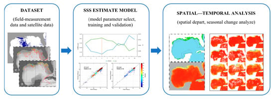
2. Materials and Methods
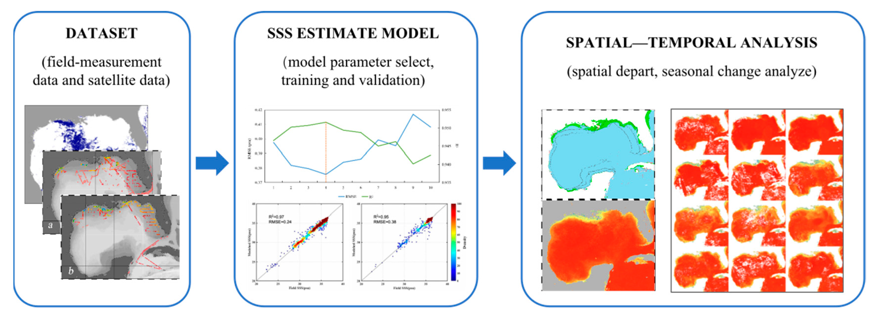
2.1. Study Area
2.2. Field Data
2.3. Satellite Data
2.4. Method
2.4.1. Cubist
2.4.2. Other Compassion Methods
3. Results
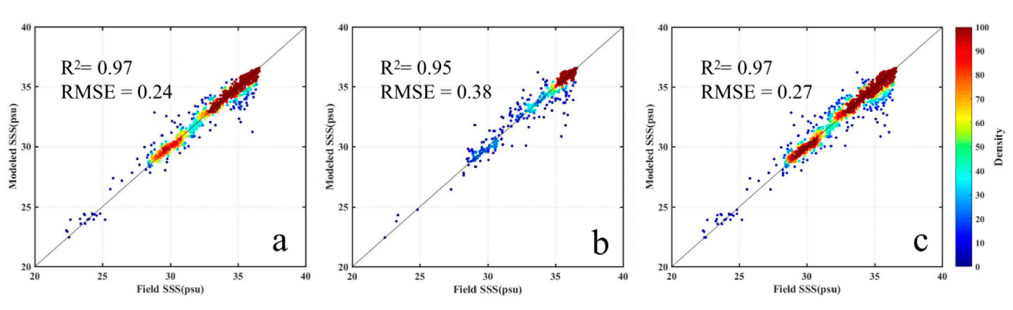
3.1. Model Performance
3.2. Rule Accuracy Validation
4. Discussion
4.1. Rule-Based GOM Partition
4.2. Seasonal Variations of Surface Salinity
4.3. Model Evaluation for Various Cases
5. Conclusions
Author Contributions
Funding
Acknowledgments
Conflicts of Interest
References
- Sun, D.; Su, X.; Qiu, Z.; Wang, S.; Mao, Z.; He, Y. Remote Sensing Estimation of Sea Surface Salinity from GOCI Measurements in the Southern Yellow Sea. Remote Sens. 2019, 11, 775. [Google Scholar] [CrossRef]
- Klemas, V. Remote Sensing of Sea Surface Salinity: An Overview with Case Studies. J. Coast. Res. 2011, 276, 830–838. [Google Scholar] [CrossRef]
- Rao, R.R.; Sivakumar, R. Seasonal variability of sea surface salinity and salt budget of the mixed layer of the north Indian Ocean. J. Geophys. Res. Ocean. 2003, 108, 9. [Google Scholar] [CrossRef]
- Fennel, K.; Hetland, R.D.; Feng, Y.S.; DiMarco, S.F. A coupled physical-biological model of the Northern Gulf of Mexico shelf: Model description, validation and analysis of phytoplankton variability. Biogeosciences 2011, 8, 1881–1899. [Google Scholar] [CrossRef]
- Xue, Z.; He, R.; Fennel, K.; Cai, W.-J.; E Lohrenz, S.; Hopkinson, C.S. Modeling ocean circulation and biogeochemical variability in the Gulf of Mexico. Biogeosciences 2013, 10, 7219–7234. [Google Scholar] [CrossRef]
- Le Vine, D.M.; Kao, M.; Garvine, R.W.; Sanders, T. Remote Sensing of Ocean Salinity: Results from the Delaware Coastal Current Experiment. J. Atmos. Ocean. Technol. 1998, 15, 1478–1484. [Google Scholar] [CrossRef]
- Qing, S.; Zhang, J.; Cui, T.; Bao, Y. Retrieval of sea surface salinity with MERIS and MODIS data in the Bohai Sea. Remote Sens. Environ. 2013, 136, 117–125. [Google Scholar] [CrossRef]
- Font, J.; Camps, A.; Ballabrera-Poy, J. Microwave Aperture Synthesis Radiometry: Paving the Path for Sea Surface Salinity Measurement from Space. In Remote Sensing of the European Seas; Springer International Springer: Dordrecht, The Netherlands, 2008; ISBN 9781402067716. [Google Scholar]
- Blume, H.-J.C.; Kendall, B.M. Passive Microwave Measurements of Temperature and Salinity in Coastal Zones. IEEE Trans. Geosci. Remote Sens. 1982, 394–404. [Google Scholar] [CrossRef]
- Urquhart, E.A.; Zaitchik, B.F.; Hoffman, M.J.; Guikema, S.D.; Geiger, E.F. Remotely sensed estimates of surface salinity in the Chesapeake Bay: A statistical approach. Remote Sens. Environ. 2012, 123, 522–531. [Google Scholar] [CrossRef]
- Khorram, S. Remote sensing of salinity in the San Francisco Bay Delta. Remote Sens. Environ. 1982, 12, 15–22. [Google Scholar] [CrossRef]
- Owers, D.G.; Harker, G.E.L.; Smith, P.S.D.; Tett, P. Optical Properties of a Region of Freshwater Influence (The Clyde Sea). Estuarine, Coast. Shelf Sci. 2000, 50, 717–726. [Google Scholar] [CrossRef]
- Palacios, S.L.; Peterson, T.D.; Kudela, R.M. Development of synthetic salinity from remote sensing for the Columbia River plume. J. Geophys. Res. Ocean. 2009, 114. [Google Scholar] [CrossRef]
- Hu, C.; Montgomery, E.T.; Schmitt, R.W.; Muller-Karger, F.E. The dispersal of the Amazon and Orinoco River water in the tropical Atlantic and Caribbean Sea: Observation from space and S-PALACE floats. Deep. Sea Res. Part II Top. Stud. Oceanogr. 2004, 51, 1151–1171. [Google Scholar] [CrossRef]
- Del Vecchio, R. Influence of the Amazon River on the surface optical properties of the western tropical North Atlantic Ocean. J. Geophys. Res. Ocean. 2004, 109. [Google Scholar] [CrossRef]
- Del Castillo, C.E.; Miller, R.L. On the use of ocean color remote sensing to measure the transport of dissolved organic carbon by the Mississippi River Plume. Remote Sens. Environ. 2008, 112, 836–844. [Google Scholar] [CrossRef]
- Binding, C.; Bowers, D. Measuring the salinity of the Clyde Sea from remotely sensed ocean colour. Estuarine, Coast. Shelf Sci. 2003, 57, 605–611. [Google Scholar] [CrossRef]
- Bricaud, A.; Morel, A.; Prieur, L. Absorption by dissolved organic matter of the sea (yellow substance) in the UV and visible domains1. Limnol. Oceanogr. 1981, 26, 43–53. [Google Scholar] [CrossRef]
- D’Sa, E.J.; Hu, C.; Muller-Karger, F.E.; Carder, K.L. Estimation of colored dissolved organic matter and salinity fields in case 2 waters using SeaWiFS: Examples from Florida Bay and Florida Shelf. J. Earth Syst. Sci. 2002, 111, 197–207. [Google Scholar] [CrossRef]
- Opsahl, S.; Benner, R. Distribution and cycling of terrigenous dissolved organic matter in the ocean. Nature 1997, 386, 480–482. [Google Scholar] [CrossRef]
- Kim, D.-W.; Park, Y.-J.; Jeong, J.-Y.; Jo, Y.-H. Estimation of Hourly Sea Surface Salinity in the East China Sea Using Geostationary Ocean Color Imager Measurements. Remote Sens. 2020, 12, 755. [Google Scholar] [CrossRef]
- Siegel, D.A.; Michaels, A.F. Quantification of non-algal light attenuation in the Sargasso Sea: Implications for biogeochemistry and remote sensing. Deep. Sea Res. Part II Top. Stud. Oceanogr. 1996, 43, 321–345. [Google Scholar] [CrossRef]
- Marghany, M.; Hashim, M.; Cracknell, A.P. Modelling Sea Surface Salinity from MODIS Satellite Data. In Proceedings of the Lecture Notes in Computer Science (Including Subseries Lecture Notes in Artificial Intelligence and Lecture Notes in Bioinformatics), Fukuoka, Japan, 23–26 March 2010; Springer International Springer: Berlin/Heidelberg, Germany, 2010; Volume 6016, pp. 545–556. [Google Scholar]
- Wong, M.; Lee, K.; Kim, Y.; Nichol, J.; Li, Z.; Emerson, N. Modeling of suspended solids and sea surface salinity in Hong Kong using Aqua/MODIS satellite images. Korean J. Remote Sens. 2007, 23, 1–9. [Google Scholar]
- Zhao, J.; Temimi, M.; Ghedira, H. Remotely sensed sea surface salinity in the hyper-saline Arabian Gulf: Application to landsat 8 OLI data. Estuarine, Coast. Shelf Sci. 2017, 187, 168–177. [Google Scholar] [CrossRef]
- Marghany, M.; Hashim, M. A numerical method for retrieving sea surface salinity from MODIS satellite data. Int. J. Phys. Sci. 2011. [Google Scholar] [CrossRef]
- Marghany, M. Least square algorithm for sea surface salinity retrieving from MODIS satellite data. In Proceedings of the 2009 IEEE International Conference on Signal and Image Processing Applications, Kuala Lumpur, Malaysia, 18–19 November 2009; pp. 500–503. [Google Scholar]
- Marghany, M. Simulation of Tsunami Impact on Sea Surface Salinity along Banda Aceh Coastal Waters, Indonesia. In Advanced Geoscience Remote Sensing; IntechOpen: London, UK, 2014. [Google Scholar]
- Geiger, E.F.; Grossi, M.D.; Trembanis, A.C.; Kohut, J.T.; Oliver, M.J. Satellite-derived coastal ocean and estuarine salinity in the Mid-Atlantic. Cont. Shelf Res. 2013, 63, S235–S242. [Google Scholar] [CrossRef]
- Marghany, M.; Hashim, M. Retrieving seasonal sea surface salinity from MODIS satellite data using a Box-Jenkins algorithm. In Proceedings of the 2011 IEEE International Geoscience and Remote Sensing Symposium, Sendai, Japan, 1–5 August 2011; pp. 2017–2020. [Google Scholar] [CrossRef]
- Moussa, H.; Benallal, M.A.; Goyet, C.; Lefevre, N.; El Jai, M.C.; Guglielmi, V.; Touratier, F. A comparison of Multiple Non-linear regression and neural network techniques for sea surface salinity estimation in the tropical Atlantic ocean based on satellite data. ESAIM Proc. Surv. 2015, 49, 65–77. [Google Scholar] [CrossRef]
- Rajabi-Kiasari, S.; Hasanlou, M. An efficient model for the prediction of SMAP sea surface salinity using machine learning approaches in the Persian Gulf. Int. J. Remote Sens. 2020, 41, 3221–3242. [Google Scholar] [CrossRef]
- Liu, M.; Liu, X.; Liu, D.; Ding, C.; Jiang, J. Multivariable integration method for estimating sea surface salinity in coastal waters from in situ data and remotely sensed data using random forest algorithm. Comput. Geosci. 2015, 75, 44–56. [Google Scholar] [CrossRef]
- Chen, S.; Hu, C. Estimating sea surface salinity in the northern Gulf of Mexico from satellite ocean color measurements. Remote Sens. Environ. 2017, 201, 115–132. [Google Scholar] [CrossRef]
- Medina-Lopez, E. Machine Learning and the End of Atmospheric Corrections: A Comparison between High-Resolution Sea Surface Salinity in Coastal Areas from Top and Bottom of Atmosphere Sentinel-2 Imagery. Remote Sens. 2020, 12, 2924. [Google Scholar] [CrossRef]
- Yáñez-Arancibia, A.; Day, J.W. The Gulf of Mexico: Towards an integration of coastal management with large marine ecosystem management. Ocean Coast. Manag. 2004, 47, 537–563. [Google Scholar] [CrossRef]
- Deegan, L.A.; Day, J.W.; Gosselink, J.G.; Yáñez-Arancibia, A.; Chávez, G.S.; Sánchez-Gil, P. Relationships Among Physical Characteristics, Vegetation Distribution and Fisheries Yield in Gulf of Mexico Estu-Aries. In Estuarine Variability; Elsevier: Amsterdam, Switzerland, 1986. [Google Scholar]
- Brokaw, R.J.; Subrahmanyam, B.; Morey, S.L. Loop Current and Eddy-Driven Salinity Variability in the Gulf of Mexico. Geophys. Res. Lett. 2019, 46, 5978–5986. [Google Scholar] [CrossRef]
- Fournier, S.; Lee, T.; Gierach, M.M. Seasonal and interannual variations of sea surface salinity associated with the Mississippi River plume observed by SMOS and Aquarius. Remote Sens. Environ. 2016, 180, 431–439. [Google Scholar] [CrossRef]
- Liang, Z.; Chen, S.; Yang, Y.; Zhou, Y.; Shi, Z. High-resolution three-dimensional mapping of soil organic carbon in China: Effects of SoilGrids products on national modeling. Sci. Total. Environ. 2019, 685, 480–489. [Google Scholar] [CrossRef]
- Peng, J.; Biswas, A.; Jiang, Q.; Zhao, R.; Hu, J.; Hu, B.; Shi, Z. Estimating soil salinity from remote sensing and terrain data in southern Xinjiang Province, China. Geoderma 2019, 337, 1309–1319. [Google Scholar] [CrossRef]
- Yan, F.; Shangguan, W.; Zhang, J.; Hu, B. Depth-to-bedrock map of China at a spatial resolution of 100 meters. Sci. Data 2020, 7, 1–13. [Google Scholar] [CrossRef]
- Ma, Z.; Zhou, Y.; Hu, B.; Liang, Z.; Shi, Z. Downscaling annual precipitation with TMPA and land surface characteristics in China. Int. J. Clim. 2017, 37, 5107–5119. [Google Scholar] [CrossRef]
- Dai, A.; Trenberth, K.E. Estimates of freshwater discharge from continents: Latitudinal and seasonal variations. J. Hydrome-teorol. 2002, 660–687. [Google Scholar] [CrossRef]
- Ellis, J.T.; Dean, B.J. Gulf of Mexico Processes. J. Coast. Res. 2012, 60, 6–13. [Google Scholar] [CrossRef]
- Morey, S.L.; Martin, P.J.; O’Brien, J.J.; Wallcraft, A.A.; Zavala-Hidalgo, J. Export pathways for river discharged fresh water in the northern Gulf of Mexico. J. Geophys. Res. Ocean. 2003, 108. [Google Scholar] [CrossRef]
- Morey, S.L.; Schroeder, W.W.; O’Brien, J.J.; Zavala-Hidalgo, J. The annual cycle of riverine influence in the eastern Gulf of Mexico basin. Geophys. Res. Lett. 2003, 30. [Google Scholar] [CrossRef]
- Ma, Z.; Shi, Z.; Zhou, Y.; Xu, J.; Yu, W.; Yang, Y. A spatial data mining algorithm for downscaling TMPA 3B43 V7 data over the Qinghai–Tibet Plateau with the effects of systematic anomalies removed. Remote Sens. Environ. 2017, 200, 378–395. [Google Scholar] [CrossRef]
- Malone, B.P.; Minasny, B.; Odgers, N.P.; McBratney, A.B. Using model averaging to combine soil property rasters from legacy soil maps and from point data. Geoderma 2014, 34–44. [Google Scholar] [CrossRef]
- Gordon, A.D.; Breiman, L.; Friedman, J.H.; Olshen, R.A.; Stone, C.J. Classification and Regression Trees. Biometrics 1984, 40, 874. [Google Scholar] [CrossRef]
- Fu, T.; Zhao, R.; Hu, B.; Jia, X.; Wang, Z.; Zhou, L.; Huang, M.; Li, Y.; Shi, Z. Novel framework for modelling the cadmium balance and accumulation in farmland soil in Zhejiang Province, East China: Sensitivity analysis, parameter optimisation, and forecast for 2050. J. Clean. Prod. 2021, 279, 123674. [Google Scholar] [CrossRef]
- Fu, Z.; Hu, L.; Chen, Z.; Zhang, F.; Shi, Z.; Hu, B.; Du, Z.; Liu, R. Estimating spatial and temporal variation in ocean surface pCO2 in the Gulf of Mexico using remote sensing and machine learning techniques. Sci. Total Environ. 2020, 745, 140965. [Google Scholar] [CrossRef] [PubMed]
- Kuhn, M.; Weston, S.; Keefer, C.; Coulter, N. Cubist Models for Regression; Vignette R Packag. 2016. Available online: https://mran.microsoft.com/snapshot/2016-09-15/web/packages/Cubist/vignettes/cubist.pdf (accessed on 25 February 2021).
- Oosterbaan, R.J. Frequency and Regression Analysis of Hydrologic Data. In Drainage Principles and Applications; International Institute for Land Reclamation and Improvement(ILRI): Wageningen, The Netherlands, 1994. [Google Scholar]
- Vapnik, V.N. The Nature of Statistical Learning Theory; Springer New York, Inc.: New York, NY, USA, 1995. [Google Scholar]
- Smola, A.J.; Schölkopf, B. A tutorial on support vector regression. Stat. Comput. 2004, 14, 199–222. [Google Scholar] [CrossRef]
- Vazquez, J.; Gierach, M.M.; Leben, R.R.; Tsontos, V.M. Initial results on the variability of sea surface salinity from Aquarius/SAC-D in the Gulf of Mexico. In Proceedings of the AGU Fall Meeting Abstracts, San Francisco, FL, USA, 3–7 December 2012. [Google Scholar]
- Feng, H.; VanDeMark, D.; Wilkin, J. Gulf of Maine salinity variation and its correlation with upstream Scotian Shelf currents at seasonal and interannual time scales. J. Geophys. Res. Oceans 2016, 121, 8585–8607. [Google Scholar] [CrossRef]
- Salisbury, J.E.; Campbell, J.W.; Linder, E.; David Meeker, L.; Müller-Karger, F.E.; Vörösmarty, C.J. On the seasonal correlation of surface particle fields with wind stress and Mississippi discharge in the northern Gulf of Mexico. Deep. Sea Res. Part II Top. Stud. Oceanogr. 2004, 51, 1187–1203. [Google Scholar] [CrossRef]
- Schiller, R.V.; Kourafalou, V.H.; Hogan, P.; Walker, N.D. The dynamics of the Mississippi River plume: Impact of topography, wind and offshore forcing on the fate of plume waters. J. Geophys. Res. Ocean. 2011, 116. [Google Scholar] [CrossRef]
- Wiseman, W.; Rabalais, N.; Turner, R.; Dinnel, S.; Macnaughton, A. Seasonal and interannual variability within the Louisiana coastal current: Stratification and hypoxia. J. Mar. Syst. 1997, 12, 237–248. [Google Scholar] [CrossRef]
- Feng, Y.; DiMarco, S.F.; Jackson, G.A. Relative role of wind forcing and riverine nutrient input on the extent of hypoxia in the northern Gulf of Mexico. Geophys. Res. Lett. 2012, 39. [Google Scholar] [CrossRef]


| Cruise ID | Platforms | Date Range | # of Observations |
|---|---|---|---|
| EQ17 | M/V Celebrity Equinox | 1/1/2018–1/6/2018 | 2179 |
| AS17 | M/V Allure of the Seas | 1/4/2018–1/7/2018 | 1198 |
| GU1801_Leg1 | R/V Gordon Gunter | 1/14/2018–1/22/2018 | 4178 |
| GU1801_Leg2 | R/V Gordon Gunter | 1/26/2018–2/9/2018 | 7421 |
| GU1801_Leg3 | R/V Gordon Gunter | 2/12/2018–2/27/2018 | 5428 |
| GU1801_Leg4 | R/V Gordon Gunter | 3/1/2018–3/16/2018 | 7941 |
| GU1802 | R/V Gordon Gunter | 6/24/2018–7/9/2018 | 7609 |
| GU1803-transit | R/V Gordon Gunter | 7/11/2018–7/14/2018 | 1340 |
| GU1803-Leg1 | R/V Gordon Gunter | 7/20/2018–8/3/2018 | 7196 |
| GU1803-Leg2 | R/V Gordon Gunter | 8/6/2018–8/19/2018 | 4727 |
| GU1804 | R/V Gordon Gunter | 8/23/2018–8/31/2018 | 4445 |
| GU1805-Leg1 | R/V Gordon Gunter | 9/2/2018–9/9/2018 | 3563 |
| GU1805-Leg2 | R/V Gordon Gunter | 9/11/2018–9/30/2018 | 9659 |
| EQ18 | M/V Celebrity Equinox | 1/6/2018–12/22/2018 | 872 |
| GU1806 | R/V Gordon Gunter | 11/10/2018–12/4/2018 | 10,127 |
| GM0606 | OSV Bold | 6/6/2006–6/11/2006 | 7178 |
| GU1609Leg1-3 | R/V Gordon Gunter | 9/2/2016–10/1/2016 | 10,284 |
| EQNX_20190209 | M/V Celebrity Equinox | 2/9/2019–2/16/2019 | 2270 |
| Total from all cruises | 97,615 | ||
| Total used in model development and validation | 7935 | ||
| Total used in independent validation | 7494 | ||
| Approach | RMSE (psu) | R2 | MB (psu) | MAE (psu) | |
|---|---|---|---|---|---|
| MLR [7] | Training | 1.00 | 0.64 | 0.00 | 0.61 |
| Validation | 1.04 | 0.63 | 0.04 | 0.63 | |
| MNR [31] | Training | 0.78 | 0.78 | 0.00 | 0.43 |
| Validation | 0.90 | 0.72 | 0.04 | 0.44 | |
| SVM [32] | Training | 0.38 | 0.85 | 0.00 | 0.18 |
| Validation | 0.39 | 0.84 | 0.02 | 0.19 | |
| Cubist (this study) | Training | 0.24 | 0.97 | 0.00 | 0.10 |
| Validation | 0.38 | 0.95 | −0.02 | 0.16 | |
| MPNN [34] | Training | 0.62 | 0.86 | 0.00 | 0.33 |
| Validation | 0.67 | 0.85 | 0.00 | 0.35 |
| Rule | Conditions | Data Range | Equation | Count | |||||
|---|---|---|---|---|---|---|---|---|---|
| Rrs412 | Rrs443 | Rrs488 | Rrs555 | Rrs667 | SST | ||||
| 1 | Rrs(412) ≤ 0.003746 & Rrs(555) > 0.001552 | −0.001744–0.003746 | −0.000418–0.00578 | 0.000846–0.009736 | 0.001556–0.008024 | 0.000066–0.003372 | 18.28–32.15 | 42.01913 + 2374 ∗ Rrs(412) – 2843 ∗ Rrs(443) + 1107 ∗ Rrs(488) – 948 ∗ Rrs(555) − 0.329 ∗ SST | 539 |
| 2 | Rrs(412) > 0.003746 & SST > 28.98 | 0.003788–0.016226 | 0.003156–0.014352 | 0.002262–0.018128 | 0–0.011534 | −0.000324–0.000924 | 28.99–32.53 | 40.31452 + 271 ∗ Rrs(412) − 447 ∗ Rrs(555) − 0.218 ∗ SST − 113 ∗ Rrs(443) + 88 ∗ Rrs(488) | 870 |
| 3 | Rrs(412) ≤ 0.003746 & Rrs(555) ≤ 0.001552 | −0.001438–0.003744 | −0.000056–0.004428 | 0.000882–0.004028 | 0.000112–0.001548 | −0.000292–0.000366 | 20.25–30.75 | 39.16627 − 501 ∗ Rrs(555) + 240 ∗ Rrs(412) + 348 ∗ Rrs(488) + 261 ∗ Rrs(443) − 0.227 ∗ SST | 367 |
| 4 | Rrs(412) > 0.003746 & SST ≤ 28.98 | 0.003746–0.030036 | 0.003124–0.036298 | 0.003226–0.044100 | 0.000086–0.028062 | −0.000650–0.010122 | 18.27–28.98 | 38.57491 − 0.105 ∗ SST − 150 ∗ Rrs(555) + 102 ∗ Rrs(488) − 37 ∗ Rrs(443) + 27 ∗ Rrs(412) | 4572 |
| Rule | Count | RMSE (psu) | R2 | MB (psu) | MAE (psu) |
|---|---|---|---|---|---|
| 1 | 539 | 0.51 | 0.98 | −0.03 | 0.31 |
| 140 | 0.80 | 0.97 | −0.11 | 0.48 | |
| 2 | 870 | 0.41 | 0.88 | −0.03 | 0.21 |
| 207 | 0.58 | 0.80 | −0.08 | 0.35 | |
| 3 | 367 | 0.33 | 0.95 | −0.03 | 0.17 |
| 99 | 0.69 | 0.80 | −0.04 | 0.32 | |
| 4 | 4572 | 0.10 | 0.98 | 0.00 | 0.05 |
| 1167 | 0.14 | 0.96 | 0.01 | 0.07 |
| Cruise ID | RMSE (psu) | MB (psu) | MR | Count | |
|---|---|---|---|---|---|
| GM0606 | ≤30 | 2.96 | 2.04 | 1.07 | 555 |
| >30 | 1.49 | −0.02 | 1.00 | 2208 | |
| 1.88 | 0.40 | 1.02 | 2763 | ||
| GU1609Leg1-3 | ≤30 | 3.01 | 0.91 | 1.03 | 221 |
| >30 | 1.53 | 0.09 | 1.00 | 3597 | |
| 1.65 | 0.14 | 1.00 | 3818 | ||
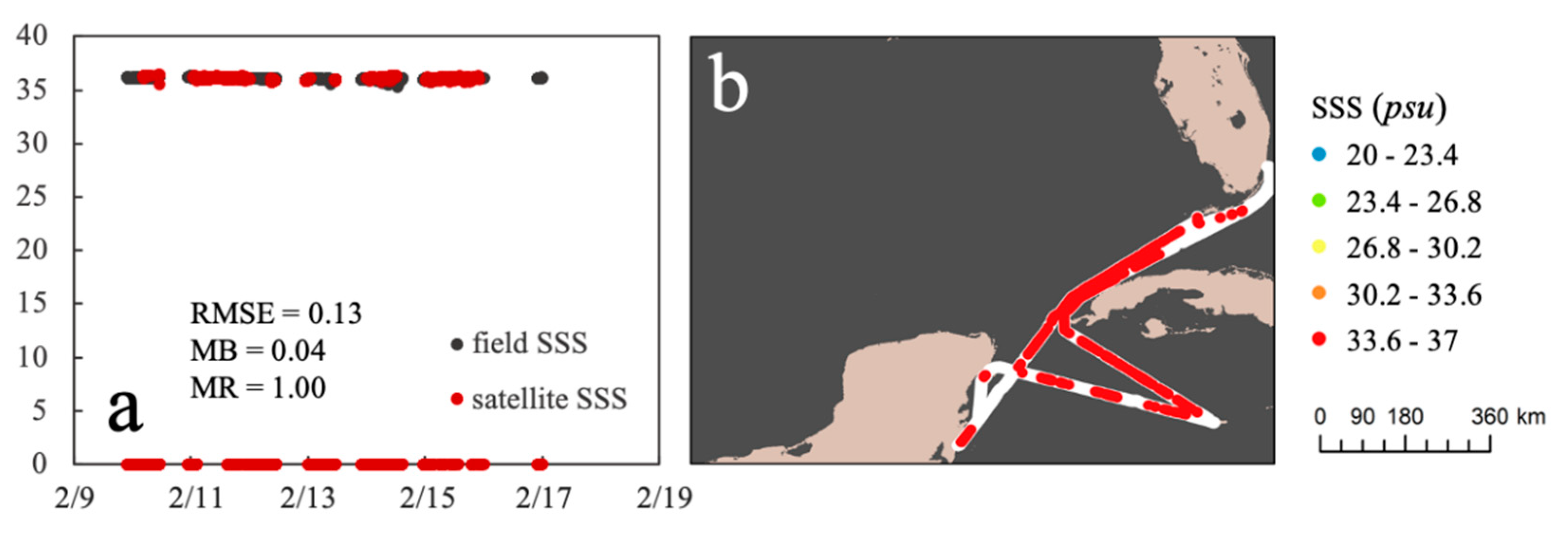
| M2019 | >30 | 0.13 | 0.04 | 1.00 | 914 |
| Total | ≤30 | 2.98 | 1.72 | 1.06 | 776 |
| >30 | 1.41 | 0.05 | 1.00 | 6719 | |
| 1.64 | 0.22 | 1.01 | 7495 |
| Approach | RMSE (psu) | MB (psu) | MR | |
|---|---|---|---|---|
| MLR | ≤30 | 4.13 | 3.46 | 1.13 |
| >30 | 1.01 | −0.12 | 1.00 | |
| 2.06 | 0.60 | 1.02 | ||
| MNR | ≤30 | 4.57 | 4.25 | 1.16 |
| >30 | 1.53 | 0.14 | 1.01 | |
| 2.46 | 0.96 | 1.04 | ||
| SVM | ≤30 | 5.13 | 4.63 | 1.17 |
| >30 | 1.37 | 0.07 | 1.00 | |
| 2.60 | 0.98 | 1.04 | ||
| MPNN | ≤30 | 3.69 | 3.02 | 1.11 |
| >30 | 1.19 | −0.33 | 0.99 | |
| 1.97 | 0.34 | 1.02 |
| Approach | RMSE (psu) | MB (psu) | MR | |
|---|---|---|---|---|
| MLR | ≤30 | 2.81 | −2.74 | 1.14 |
| >30 | 1.34 | 0.41 | 1.01 | |
| 1.46 | 0.23 | 1.02 | ||
| MNR | ≤30 | 3.27 | −2.81 | 1.14 |
| >30 | 1.51 | 0.20 | 1.00 | |
| 1.67 | 0.02 | 1.01 | ||
| SVM | ≤30 | 5.47 | 4.80 | 1.19 |
| >30 | 1.06 | 0.13 | 1.00 | |
| 1.67 | 0.40 | 1.02 | ||
| MPNN | ≤30 | 4.70 | 3.66 | 1.15 |
| >30 | 1.17 | 0.21 | 1.01 | |
| 1.60 | 0.41 | 1.02 |
| Approach | RMSE (psu) | MB (psu) | MR | |
|---|---|---|---|---|
| MLR | >30 | 0.54 | −0.15 | 1.00 |
| MNR | >30 | 0.29 | 0.08 | 1.00 |
| SVM | >30 | 0.19 | 0.06 | 1.00 |
| MPNN | >30 | 0.18 | 0.06 | 1.00 |
Publisher’s Note: MDPI stays neutral with regard to jurisdictional claims in published maps and institutional affiliations. |
© 2021 by the authors. Licensee MDPI, Basel, Switzerland. This article is an open access article distributed under the terms and conditions of the Creative Commons Attribution (CC BY) license (http://creativecommons.org/licenses/by/4.0/).
Share and Cite
Fu, Z.; Wu, F.; Zhang, Z.; Hu, L.; Zhang, F.; Hu, B.; Du, Z.; Shi, Z.; Liu, R. Sea Surface Salinity Estimation and Spatial-Temporal Heterogeneity Analysis in the Gulf of Mexico. Remote Sens. 2021, 13, 881. https://doi.org/10.3390/rs13050881
Fu Z, Wu F, Zhang Z, Hu L, Zhang F, Hu B, Du Z, Shi Z, Liu R. Sea Surface Salinity Estimation and Spatial-Temporal Heterogeneity Analysis in the Gulf of Mexico. Remote Sensing. 2021; 13(5):881. https://doi.org/10.3390/rs13050881
Chicago/Turabian StyleFu, Zhiyi, Fangfang Wu, Zhengliang Zhang, Linshu Hu, Feng Zhang, Bifeng Hu, Zhenhong Du, Zhou Shi, and Renyi Liu. 2021. "Sea Surface Salinity Estimation and Spatial-Temporal Heterogeneity Analysis in the Gulf of Mexico" Remote Sensing 13, no. 5: 881. https://doi.org/10.3390/rs13050881
APA StyleFu, Z., Wu, F., Zhang, Z., Hu, L., Zhang, F., Hu, B., Du, Z., Shi, Z., & Liu, R. (2021). Sea Surface Salinity Estimation and Spatial-Temporal Heterogeneity Analysis in the Gulf of Mexico. Remote Sensing, 13(5), 881. https://doi.org/10.3390/rs13050881