Article

Fusion of GF and MODIS Data for Regional-Scale Grassland Community Classification with EVI2 Time-Series and Phenological Features

1
School of Geoscience, Yangtze University, Wuhan 430100, China
2
Aerospace Information Research Institute, Chinese Academy of Sciences, Beijing 100094, China
3
Research Center for Remote Sensing Information and Digital Earth, College of Computer Science and Technology, Qingdao University, Qingdao 266071, China
4
Agricultural Comprehensive Development Office, Dongsheng District, Ordos City 017000, China
*
Author to whom correspondence should be addressed.
Remote Sens. 2021, 13(5), 835; https://doi.org/10.3390/rs13050835
Submission received: 14 January 2021 / Revised: 16 February 2021 / Accepted: 19 February 2021 / Published: 24 February 2021
(This article belongs to the Special Issue Remote Sensing Applications in Vegetation Classification)

Abstract

:
Satellite-borne multispectral data are suitable for regional-scale grassland community classification owing to comprehensive coverage. However, the spectral similarity of different communities makes it challenging to distinguish them based on a single multispectral data. To address this issue, we proposed a support vector machine (SVM)–based method integrating multispectral data, two-band enhanced vegetation index (EVI2) time-series, and phenological features extracted from Chinese GaoFen (GF)-1/6 satellite with (16 m ) spatial and (2 d) temporal resolution. To obtain cloud-free images, the Enhanced Spatial and Temporal Adaptive Reflectance Fusion Model (ESTARFM) algorithm was employed in this study. By using the algorithm on the coarse cloudless images at the same or similar time as the fine images with cloud cover, the cloudless fine images were obtained, and the cloudless EVI2 time-series and phenological features were generated. The developed method was applied to identify grassland communities in Ordos, China. The results show that the Caragana pumila Pojark, Caragana davazamcii Sanchir and Salix schwerinii E. L. Wolf grassland, the Potaninia mongolica Maxim, Ammopiptanthus mongolicus S. H. Cheng and Tetraena mongolica Maxim grassland, the Caryopteris mongholica Bunge and Artemisia ordosica Krasch grassland, the Calligonum mongolicum Turcz grassland, and the Stipa breviflora Griseb and Stipa bungeana Trin grassland are distinguished with an overall accuracy of 87.25%. The results highlight that, compared to multispectral data only, the addition of EVI2 time-series and phenological features improves the classification accuracy by 9.63% and 14.7%, respectively, and even by 27.36% when these two features are combined together, and indicate the advantage of the fine images in this study, compared to 500 m moderate-resolution imaging spectroradiometer (MODIS) data, which are commonly used for grassland classification at regional scale, while using 16 m GF data suggests a 23.96% increase in classification accuracy with the same extracted features. This study indicates that the proposed method is suitable for regional-scale grassland community classification.

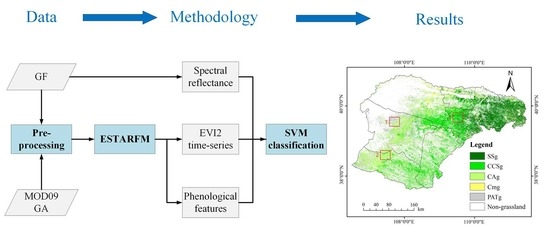
Graphical Abstract

1. Introduction

Grassland covers about 40% of the Earth’s surface [1]. In China, grassland covers about 3.93 × 10 6 km2, accounting for 41.7% of the total land area [2]. It is a renewable source for livestock production, helps ecological stability, and produces wealth for humans [3]. Generally, grassland classification plays an essential role in sustainable grass production and protection [4]. The field survey is a common approach for the classification of grassland. However, it is a laborious and time-consuming method [5,6,7]. Alternatively, remote sensing (RS) provides an inexpensive, convenient, and effective technology for grassland classification [8]. RS-based unmanned aerial vehicles (UAV) have acquired hyperspectral or high-spatial resolution datasets which are well known, and precise methods for classification of grassland over the small area can be implemented [9,10,11,12]. In contrast, a satellite-borne multispectral dataset is more suitable for the regional scale [13,14,15].
However, it is difficult to accurately classify grassland communities using only satellite-borne multispectral data due to the similar spectral features of different grassland communities [2,16]. The vegetation index (VI), such as the Normalized Difference Vegetation Index (NDVI) and Enhanced Vegetation Index (EVI), is an important indicator for grassland classification [17,18]. Compared with single-phase classification, classification with multiple-phase VI data usually obtains more precise results [19,20,21]. For example, Wen et al. (2010) combined the EVI time-series derived from moderate-resolution imaging spectroradiometer (MODIS) images in combination with Digital Elevation Model (DEM) data to classify meadow steppe, typical steppe, desert steppe, alpine meadow steppe, alpine typical steppe, and shrub herbosa in Tibet, China using the Iterative Selforganizing Data Analysis (ISODATA) classifier [22]. Schuster et al. (2015) used time-series NDVI data extracted from the RapidEye images and discriminated seven grassland types in a nature reserve in northeastern Germany using a support vector machine (SVM) classifier with an accuracy of 91.7% [23]. In addition to VI, the phenological feature of vegetation is another piece of information that can be used for grassland classification [24,25,26]. Grassland communities are specific compositional structures that have evolved as a result of natural environmental influences, such as temperature and precipitation, and thus different communities will exhibit different growth rhythms [27,28]. Wang et al. (2015) used NDVI data and phenological features to perform the classification of grassland. Compared with that without phenological features, the classification accuracy was improved by 13.7% [29].
The accurate acquisition of a time-series dataset requires a short revisit cycle of the satellite. Previous studies suggested that the MODIS dataset is suitable for time-series analysis due to high temporal resolution [30,31]. However, using the MODIS dataset with low spatial resolution for grassland classification is problematic, due to it containing many mixed pixels [32]. Compared to MODIS, the Chinese GaoFen (GF)-1/6 networking satellite’s wide field view (WFV) data with 16 m spatial and 2 d temporal resolution will be more feasible for grassland classification [33]. However, few studies have been conducted using these data for grassland classification.
The GF-1/6 satellite consists of two satellites, namely GF-1 and GF-6, which were launched on 26 April 2013 and 2 June 2018, respectively. The GF-1/6 satellite, with a 2 d temporal resolution [34], provides a great facility for the acquisition of time-series data. In addition, the free WFV data, with spatial resolution of 16 m and 800 km swath width, allow for a relatively large area of vegetation monitoring. However, using GF data is still subject to some difficulties, such as missing data [35] and cloud cover [36]. Spatio-temporal fusion (STF) is a suitable solution for these issues [37]. Currently, several STF algorithms have been developed, and among these algorithms, the enhanced spatial and temporal adaptive reflectance fusion model (ESTARFM) is universally used for various data, such as GF and MODIS satellite images [38], Advanced Spaceborne Thermal Emission and Reflection Radiometer (ASTER) and MODIS [39], RapidEye and MODIS [40], Sentinel-2 and MODIS [41], etc. Previous studies have indicated that this algorithm performs well, especially in the red and near-infrared bands [42].
The ESTARFM algorithm was improved from the spatial and temporal adaptive reflectance fusion model (STARFM) [43]. It considers the heterogeneity of the pixels, and introduces a conversion coefficient for the reflectance of pure pixels and mixed pixels, which improves the fusion accuracy of the model in regions of high heterogeneity [44]. To derive a high-spatial resolution image, a base high-temporal but low-spatial resolution image, two days of high-temporal but low-spatial resolution and high-spatial but low-temporal resolution images are needed by ESTARFM.
The Inner Mongolian steppe is vast and is an important part of the Eurasia Steppe [2]. Ordos, with 5.9 × 10 4 km2 of grassland, is located in the south of Inner Mongolia. There are numerous types of grassland communities [45]. Therefore, the study on the classification of grassland communities at the regional scale is important for the conservation and utilization of grassland resources in the region.
In this study, we attempt to propose a SVM–based method for regional-scale grassland community classification integrating two-band enhanced vegetation index (EVI2) [46] time-series, phenological features and GF multispectral data. The objectives of this study are to: (1) test the applicability of the ESTARFM algorithm in GF-1/6 satellite data; (2) verify whether the addition of phenological features and EVI2 time-series are capable of improving the accuracy of grassland community classification; (3) verify the advantage of GF-1/6 satellite data in grassland community classification; and (4) map the spatial distribution of the five main grassland communities in Ordos at 16 m spatial resolution.

2. Study Area and Data

2.1. Study Area

The study was conducted in the Ordos region, in which the Ordos Prefecture consists of two parts: grassland and desert. Ordos is located in the Inner Mongolia province of China, and the total area is approximately 8.7 × 10 4 km2 (37.59 ° to 40.86 ° N, 106.71 ° to 111.46 ° E), of which about 70% is grassland (Figure 1). The area’s climate is temperate semi-arid, with an mean annual temperature and precipitation of 6.2 ° C and 348.3 mm, respectively. Winter is cold, with a daily minimum temperature reaching 31.4 ° C , and summer is hot, with a daily maximum temperature reaching 38 ° C . Precipitation mostly occurs in July, August, and September, which constitutes about 70% of the annual total precipitation.
According to the fieldwork and previous studies [48,49], within the study area, there are five main grassland communities, namely (1) Caragana pumila Pojark, Caragana davazamcii Sanchir, Salix schwerinii E. L. Wolf grassland (hereafter CCSg), (2) Potaninia mongolica Maxim, Ammopiptanthus mongolicus S. H. Cheng, Tetraena mongolica Maxim grassland (hereafter PATg), (3) Caryopteris mongholica Bunge and Artemisia ordosica Krasch grassland (hereafter CAg), (4) Calligonum mongolicum Turcz grassland (hereafter Cmg), and (5) Stipa breviflora Griseb and Stipa bungeana Trin grassland (hereafter SSg). Each community contains several companion species (Table 1).

2.2. GF-1, GF-6 Data and Pre-Processing

GF-1 and GF-6 are both satellites of China High-Resolution Earth Observation System (HDEOS) [50]. They carry WFV cameras with the same spatial resolution of 16 m and cover the visible to the near-infrared spectral regions (Table 2). Meanwhile, the GF-1/6 satellite has achieved a 2 d revisit cycle of China, which has dramatically improved RS data acquisition’s scale and timeliness [51]. In this study, 23 phases of images from 13 December 2018 to 3 December 2019, a total of 64 GF-1 and 30 GF-6 images (as shown in Table 3), were employed for the grassland community classification.
The following pre-processing procedures were performed on the GF dataset: (a) radiometric calibration, (b) atmospheric correction using the Fast Line-of-sight Atmospheric Analysis of Spectral Hypercubes (FLAASH) model, (c) geometric correction, (d) reprojection, and (e) resampling. The digital numbers were converted into real reflectance values for the land surfaces by the above processes, atmosphere effects were eliminated, and the exact geometric correction ensured accuracy within 0.5 pixels. All images were transformed in the WGS84 reference coordinate system, and resampled at 16 m spatial resolution using the bilinear interpolation method.

2.3. MODIS MOD09GA Dataset and Pre-Processing

The MOD09GA dataset provides seven spectral channels ranging from visible to infrared bands with a spatial resolution of 500 m and temporal resolution of 1 d, which is corrected for atmospheric effects [52]. The MOD09GA dataset covering the study area (Tiles h26v04 and h26v05) was downloaded from the National Aeronautics and Space Administration (NASA) website (https://ladsweb.nascom.nasa.gov/search, accessed on 10 October 2020). As the data were corrected for atmospheric effects, we only reprojected the data to the WGS84 reference coordinate system and resampled them to 16 m using the MODIS Reprojection Tool (MRT). Then we geo-rectified the MOD09GA to the GF images.

2.4. Reference Data

The ground truth field survey was conducted in July 2019, when the Ordos’ grassland was at peak growing season. Combining previous studies, the vegetation type map of Ordos [48], and Google Earth images, a set of samples for each of the five communities were collected (Table 4). Given that the Ordos did not have dramatic changes in land-cover types between 2017 and 2019, we masked the non-grassland area out by using the 10 m land-cover map of Ordos in 2017 [47], to eliminate the interference of other land-use types in this study.

3. Methods

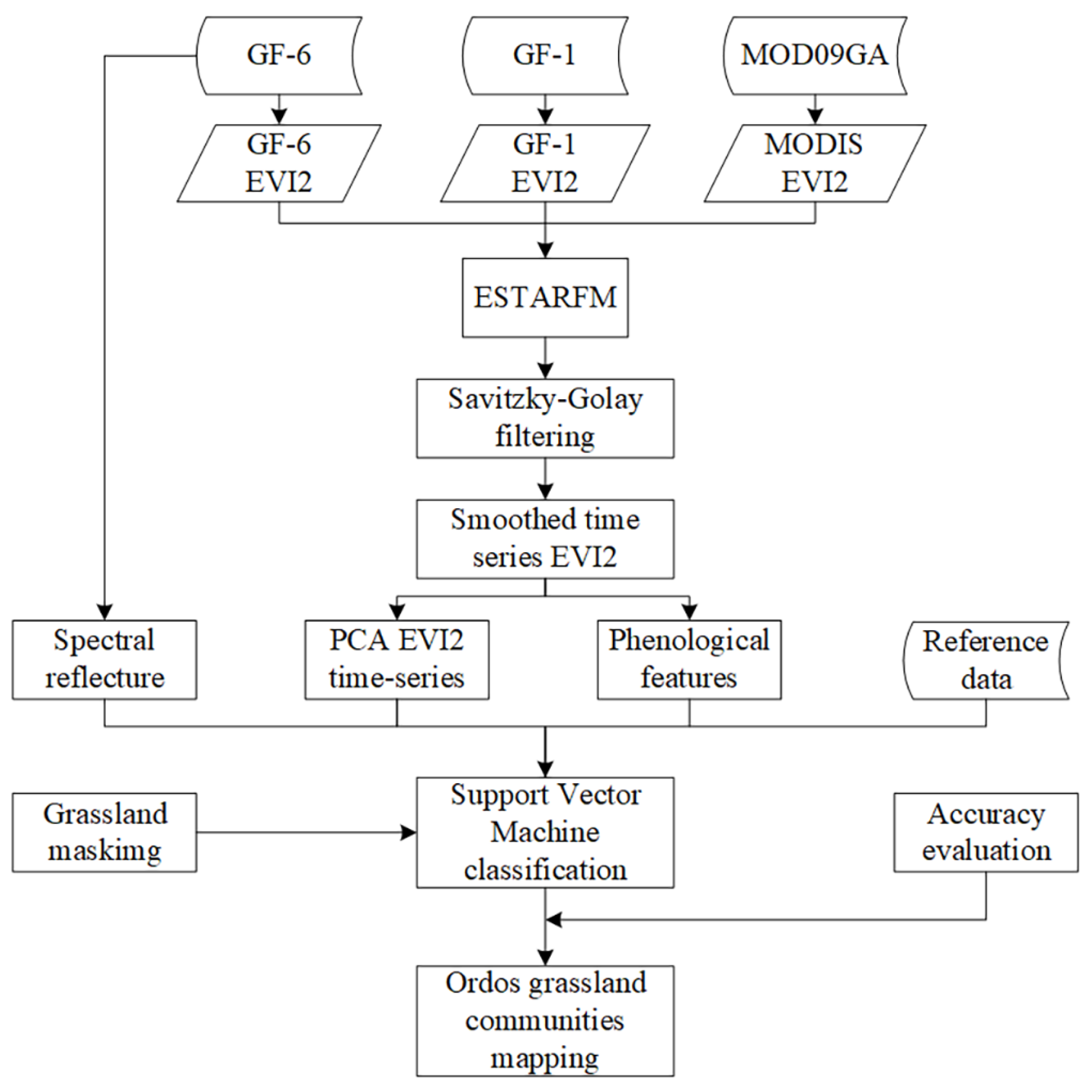
The flowchart of the grassland community classification in the study area is presented in Figure 2. The proposed method has four main steps. Firstly, the EVI2 was calculated from the GF and the MOD09GA dataset, respectively. Secondly, the fused cloudless images were generated by the ESTARFM algorithm to replace the original images with cloud cover (described in Section 3.1). Thirdly, after the Savitzky–Golay smoothing, six phenological features were derived from the fused EVI2 time-series, then the key information of fused EVI2 time-series (hereafter PCA EVI2 time-series) was extracted using the principle component analysis (PCA) algorithm. After that, the non-grassland land types were masked out (as described in Section 2.4). Finally, grassland community classification was performed based on the SVM classifier, integrating the PCA EVI2 time-series, phenological features, and GF multispectral data.

3.1. Generation of Cloudless EVI2 Time-Series by the Enhanced Spatial and Temporal Adaptive Reflectance Fusion Model (ESTARFM) Algorithm

Due to frequent cloud cover in the study area, a large proportion of the GF data were unusable. Thus, we performed the ESTARFM algorithm for the GF and MODIS images to capture the cloudless EVI2 time-series. Although the ESTARFM algorithm is rigorous, it still yields some errors during the process of fusion, which would reduce classification accuracy. Thus, we only applied it to the areas of the images with cloud cover, rather than the entire image.
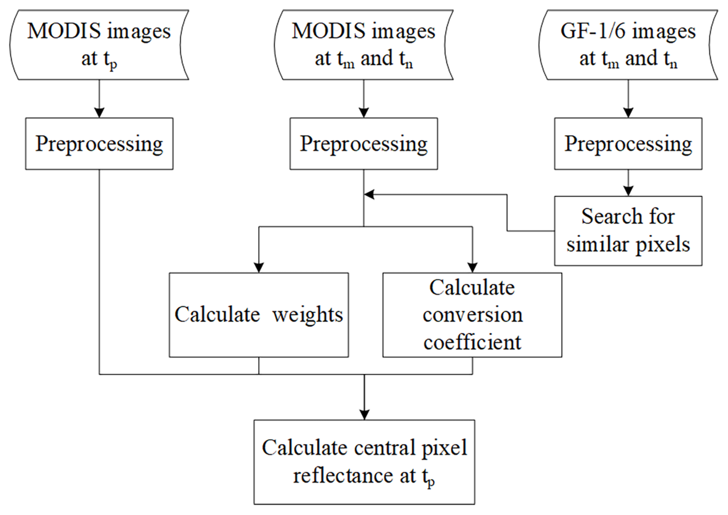
The ESTARFM algorithm was modified from the spatial and temporal adaptive reflectance fusion model (STARFM) [43], and the flowchart of it is shown in Figure 3. It considers the heterogeneity of the pixels, adjusts the assignment method, and introduces a conversion coefficient to improve the fusion results, which improves the fusion accuracy, especially in the regions with considerable heterogeneity [44]. After aligning two images, it is assumed that the difference in reflectance between the GF and MODIS pixels is only caused by the systematic biases. Therefore, the linear relationship between the reflectances of the MODIS and GF data is as shown in Equation (1)
F x , y , t k , B = a × C x , y , t k , B + b
where F and C represent the reflectances of GF and MODIS data, respectively; ( x , y ) represents the pixel’s location; t k is the acquisition time of the image; B is the band of image; and a and b are the coefficients of the linear equation.
If there are two pairs of GF and MODIS images for the same area in time t m and t n , respectively, and the type of land cover and sensor calibration do not change significantly during the period, then Equation (1) can be written as Equation (2) at t m and Equation (3) at t n
F x , y , t m , B = a × C x , y , t m , B + b
F x , y , t n , B = a × C x , y , t n , B + b
From Equations (2) and (3), Equation (4) can be obtained:
F x , y , t n , B = a × C x , y , t n , B C x , y , t m , B + F x , y , t m , B
However, many pixels of the MODIS images are mixed pixels due to its low spatial resolution; thus, the reflectance relationship between the GF and MODIS data may not exist as described in Equation (4). Therefore, the linear mixture model is required to denote the reflectance relationship between them:
C x , y , t m , B = i = 1 M f i 1 a F x , y , t m , B b a + ε C x , y , t n , B = i = 1 M f i 1 a F x , y , t n , B b a + ε
where f i is the fraction of each type of land cover in the mixed pixels, ε is the residual error, and M is the total number of endmembers (all the GF pixels contained within the mixed MODIS pixels). It is assumed that the change in the reflectance of each endmember is linear from t m to t n :
F x , y , t n , B = g i × Δ t + F x , y , t m , B
where Δ t = t n t m and g i is the rate of change of the kth endmember, which is assumed to be stable during this period. Then, from Equations (5) and (6), we can get the change in MODIS reflectance within this time:
C x , y , t n , B C x , y , t m , B = Δ t i = 1 M f i g i a
If the reflectance of the kth endmember at date t m and t n can obtained, Equation (6) can be written as:
Δ t = F x , y , t n , B F x , y , t m , B g k
Integrating Equation (8) into Equation (7), we obtain the ratio of the change in reflectance of the kth endmember to the change in reflectance of a coarse pixel, v k , which is called the conversion coefficient:
F x , y , t n , B F x , y , t m , B C x , y , t n , B C x , y , t m , B = g k i = 1 M f i g i a = v k
Then, Equation (4) can be rewritten as follows:
F x , y , t n , B = v k × C x , y , t n , B C x , y , t m , B + F x , y , t m , B
However, using only a single pixel’s information to fuse the reflectance of GF data is not accurate enough, and making full use of the information of adjacent pixels can obtain higher fusion accuracy [43]. The ESTARFM algorithm uses the search window of size w to search for similar pixels (adjacent pixels with the same type of land cover as the central pixel) within the window and calculates the weighted average of the values of similar pixels. Then, the GF images’ reflectance of the central pixel ( x w \ 2 , y w \ 2 ) at date t n can be calculated as:
F x w \ 2 , y w \ 2 , t n , B = i = 1 N W i × v i × C x i , y i , t n , B C x i , y i , t m , B + F x w \ 2 , y w \ 2 , t m , B
where N is the number of similar pixels, including the central pixel, ( x i , y i ) are the ith similar pixel, W i and v i is the weight and the conversion coefficient of the ith similar pixel, respectively. W i is determined by the distance between the ith similar pixel and the central pixel, and the spectral similarity between GF and MODIS pixel. The spectral similarity is determined by the correlation coefficient between the ith similar pixel and its corresponding MODIS pixel as follows:
R i = E F i E F i C i E C i D F i · D C i
where F i and C i are the datasets of pixels corresponding to GF and MODIS data, respectively, and D( F i ), D( C i ), E( F i ) and E( C i ) are the corresponding variance and expectation values, respectively.
The distance d i between the ith similar pixel and central pixel can be calculated as follows:
d i = 1 + x w \ 2 x i 2 + y w \ 2 y i 2 ( w \ 2 )
where w is the size of the search window.
Combining Equations (12) and (13), a synthetic index S i can be calculated that combines spectral similarity and d i as follows:
S i = ( 1 R i ) × d i
and the weight w i is calculated by the normalized reciprocal of S i as:
w i = 1 \ S i \ i = 1 N 1 \ S i
Since this study is mainly based on the EVI2 time-series, to reduce the computational cost, we used the ESTARFM algorithm for EVI2 instead of using it for raw data before calculating to obtain EVI2. The 2-band enhanced vegetation index (EVI2), which bears a strong resemblance to EVI [53], was derived from raw data using the following formula:
E V I 2 = 2.5 × ρ N i r ρ R e d ρ N i r + 2.4 × ρ R e d + 1
where ρ N i r and ρ R e d represent the reflectance values in the near-infrared and red bands, respectively.
After calculating EVI2, the ESTARFM algorithm was performed to fuse the region’s spectral reflectance with heavy cloud cover. The pre-processing steps for the fusion of the GF and MODIS data with the ESTARFM algorithm are as follows: Step 1, the MODIS EVI2 images were resampled to 16 m spatial resolution as the GF EVI2 images using the bilinear interpolation method. Step 2, we chose the GF EVI2 images as a reference, geo-rectified the MODIS EVI2 to the GF images. Step 3, the MODIS EVI2 images were cropped by the GF images, ensuring they were the exact same size. Finally, the ESTARFM algorithm was performed on the areas of the GF EVI2 images with heavy cloud cover.

3.2. Reconstruction of Smoothed EVI2 Time-Series

With fused EVI2 time-series, six phenological features were extracted from them. However, although the influence of cloud cover on GF images was eliminated by using the algorithm ESTARFM, the EVI2 time-series data still contained measurement errors and signal noise. Thus, it is consequential to reconstruct the EVI2 time-series before deriving the phenological parameters precisely. In this study, the Savitzky–Golay (S–G) filter, proposed by Savitzky and Golay (1964), was applied to smooth EVI2 time-series using the TIMESAT 3.3 program. It is a filtering algorithm based on the least-squares convolutional fitting of local polynomials. It applies a least-squares fit to an Nth-order polynomial by selecting some points near the original data and then calculates the average value of that point through that polynomial. It is essentially a weighted average of the original series, with the weights depending on the polynomial of the least-squares fit within the filter window. The formula of S–G filter is as follows [54]:
Y j * = i = n i = n C i Y j + 1 N
where Y j * , Y j + 1 , m, and C i denote the filtered data, the original data, the window’s width, and the filtered coefficient, respectively. N is the number of convolutions and numerically equals 2 n + 1 times the filter window width.
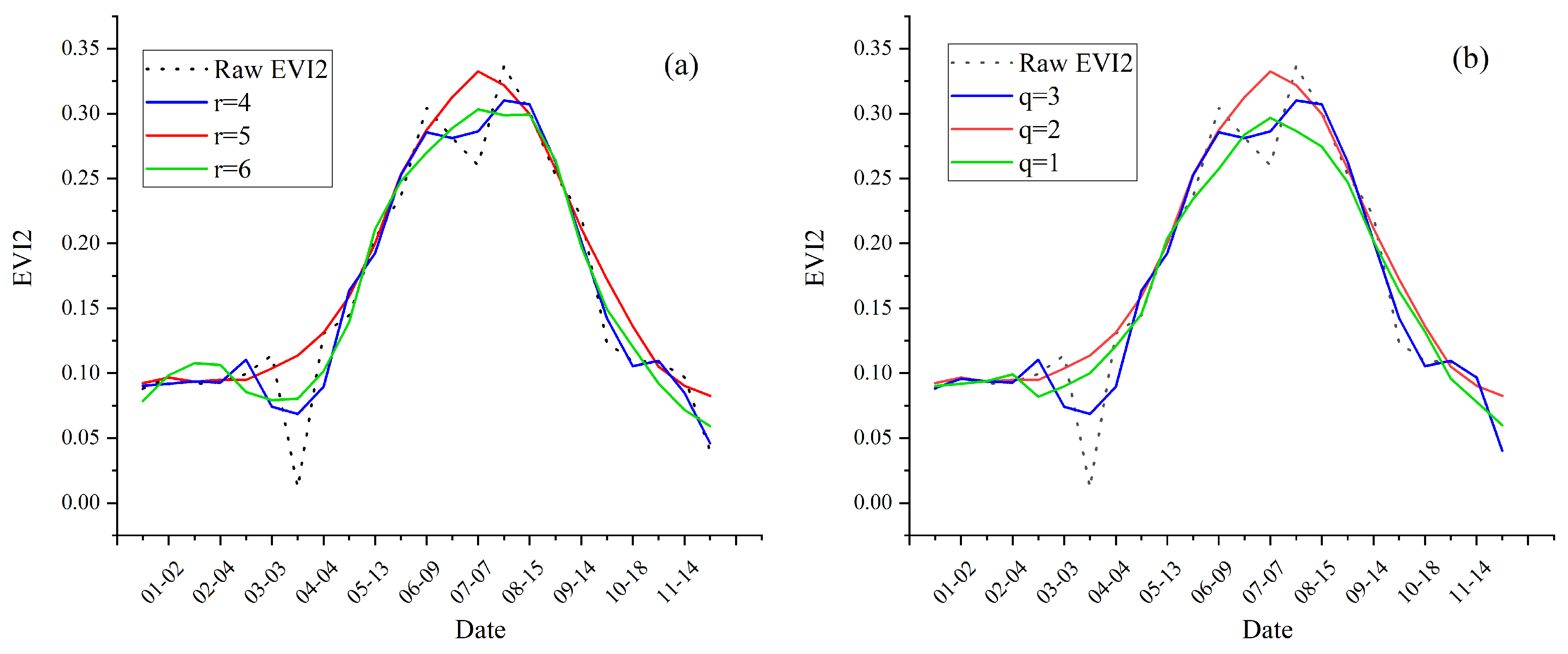
This filter is affected by two parameters: the sliding window size r and the polynomial order q. The larger the sliding window size, the more data will be involved in the fit, and the smoother the fit result will be; otherwise, more details of the original curve will be retained. The lower-order smoothing works well for the polynomials but increases the error, while the opposite results in overfitting. Based on previous studies, these two parameters can be determined according to the EVI2 observations, and q usually ranges from 2 to 4 [55]. Therefore, we tried to smooth the EVI2 time-series with different parameters of the S–G filter to find the optimal parameters for this experiment. As shown in Figure 4, the optimal smoothing effect was achieved when r was 5 and q was 2.

3.3. Extraction of Phenological Features and PCA EVI2 Time-Series

Due to the similarity of spectra among various grassland communities, it is difficult to differentiate using GF multispectral data only. Using phenological information as input data can improve the classification accuracy of different grasslands [56]. In this study, six phenological parameters were derived from the fused EVI2 time-series: (1) start of season (hereafter SOS): time for which the left edge increased to a user-defined level measured from the left minimum; (2) end of season (hereafter EOS):time for which the right edge decreased to a user-defined level measured from the right minimum level; (3) maximum of EVI2 (hereafter Max): the maximum value of each pixel in the EVI2 temporal data; (4) minimum of EVI2 (hereafter Min): the minimum value of each pixel in the temporal data; (5) mean EVI2: the mean value of each pixel in the temporal data; and (6) phenology index (hereafter PI): a measure of EVI2 seasonal variation [1]. The following equation calculates this:
( a b s ( m e a n t 1 ) + a b s ( m e a n t 2 ) + + a b s ( m e a n t n ) ) n
where a b s , m e a n , t i , and n represent absolute values, the mean of EVI2, the EVI2 value in the ist temporal phase, and the number of temporal phases of the image, respectively.
To reducing data redundancy, we performed the PCA algorithm on the EVI2 time-series. PCA is a commonly used linear dimensionality reduction method that maps higher dimensional data into a lower-dimensional space through linear projection with the expectation that the data will be most informative (i.e., have the most significant variance) in the dimension being projected. In this way, fewer data dimensions are used while retaining most of the original data’s characteristics [57]. The results of the PCA show that the first four components explained 95.07% of the variance. Thus, the first four components after the PCA transformation were included for subsequent trials.

3.4. SVM Classification and Accuracy Assessment

In recent years, the deep learning (DL) technique has shown great success in the RS classification task due to its strong learning and generalization ability [58,59]. It contains many parameters and hence requires a large number of samples for training to avoid overfitting [60]. However, sampling a large number of grassland images is challenging because it is time consuming and costly, thus limiting its usage [5,61]. Compared to DL, the SVM classifier, which is suitable for tasks with small-sample and high-dimensionality datasets [62], also has a strong generalization ability [63] and does not require assumptions about the statistical distribution of the data [64]. For these reasons, it performs well in grassland classification [65,66], and thus it was employed in this study.
To investigate the impacts of the different RS features on the classification accuracy of grassland communities, we implemented five scenarios: (1) the GF multispectral (Red, Green, Blue, and NIR bands) data only; (2) the GF multispectral data and PCA EVI2 time-series; (3) the GF multispectral data and phenological features; (4) the GF multispectral data, PCA EVI2 time-series, and phenological features; and (5) the MODIS multispectral data, PCA EVI2 time-series, and phenological features. Considering that August is the period in which the Ordos grasslands flourish the most, the GF multispectral data utilized in these scenarios are from 2 August 2019.
In this study, a compound comparison of these five scenarios was performed using the same samples (as described in Section 2.4) and the SVM classifier parameters. Four statistics, including overall accuracy, kappa coefficient, producer’s accuracy, as well as user’s accuracy, were computed to validate the classification accuracy.

4. Results

4.1. Accuracy Assessment of the ESTARFM Fusion

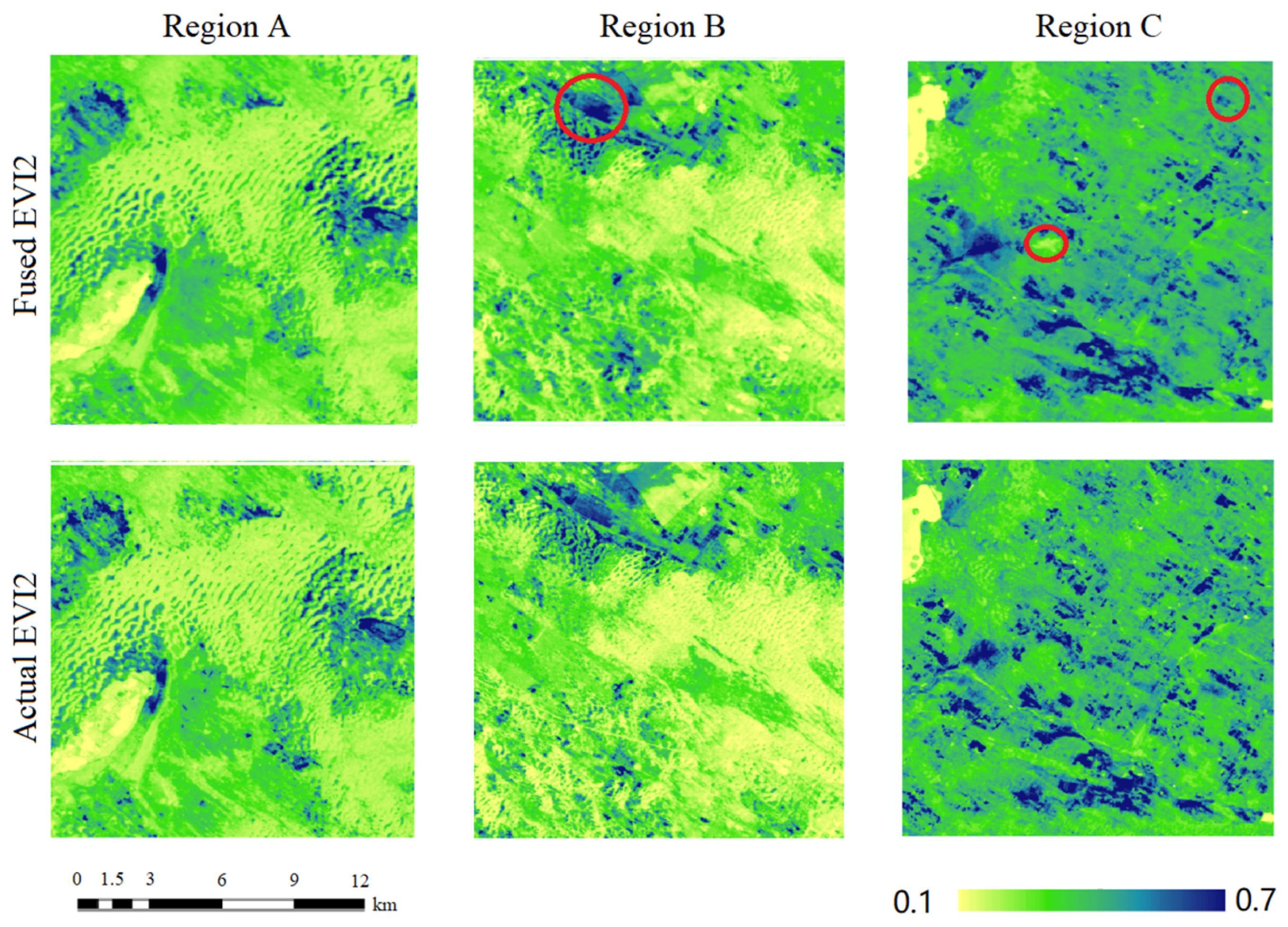
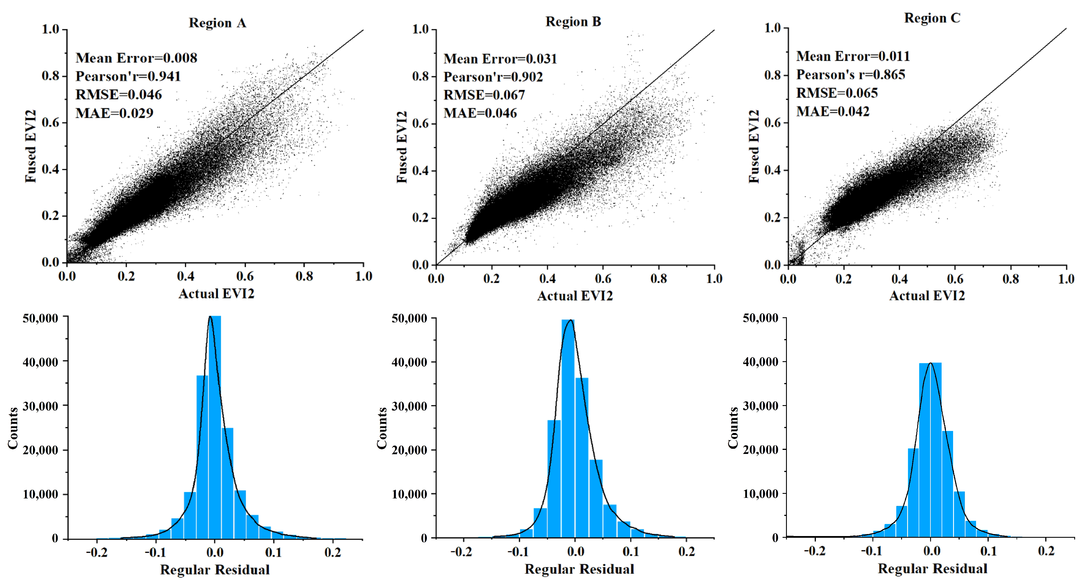
To verify that the quality of the synthetic images were reliable, we selected three representative subdomains (land cover types including grassland, bareland, cropland, water, and impervious surfaces) of 400 × 400 pixels from GF images acquired on 28 July 2019 in the study area. We compared them with the corresponding fused EVI2 image. As shown in Figure 5, the pairs of the fused and actual images are visually similar, except on some cropland (marked in Figure 5). This type of land cover would be masked out by the land-cover map of Ordos (as described in Section 2.4). Thus, it would not interfere with this study. To further quantify the fused performance, Figure 6 shows four statistics, scatter plots, and residual histograms of the pixel values for the three pairs of actual and fused EVI2 images in Figure 5. The results show that the Pearson correlation coefficient is greater than 0.86, the mean error is less than 0.03, and RMSE and MAE range from 0.046 to 0.067 and from 0.027 to 0.046, respectively. Moreover, the actual and fused EVI2 show a close adherence to the y = x line, and the residuals between them are approximately consistent with normal distributions. Therefore, the fused images are sufficiently reliable to be utilized in subsequent studies.
To demonstrate the effect of ESTARFM-based de-clouding, two examples of fusion are shown in Figure 7. According to the results, the clouds in the original images are effectively removed.

4.2. Pheonological Information Analysis

In this study, six phenological features were extracted from the EVI2 time-series of the training samples. Based on Table 5, the maximum EVI2 values differ the most across communities, ranging from 0.638 to 0.333, while minimum EVI2 values differ the least, ranging from 0.022 to 0.089. SSg has the highest mean EVI2 of 0.302. Meanwhile, the phenology index of it is also the highest, indicating its astounding degree of EVI2 fluctuation during the year. As for SOS and EOS, PATg is significantly earlier than the other communities.

4.3. Accuracy Evaluation of Different Scenarios

The overall accuracy and kappa coefficient are used to evaluate the performances of the different scenarios (see Table 6). According to the results, Scenario 1 has the lowest overall accuracy (59.89%) and kappa coefficient (0.46), revealing that it is a challenge for only RGB and NIR spectral data to differentiate grassland. Compared with Scenario 1, the overall accuracies of Scenarios 2 and 3 increase by about 9.63% and 14.7%, respectively, demonstrating that the inclusion of either phenological features or PCA EVI2 time-series improves the classification accuracy. When the two features are combined, Scenario 4 achieves the highest accuracy of 87.25%. The results prove that integrating PCA EVI2 time-series and phenological features dramatically boosts the classification accuracy compared to using one or the other alone. However, it should be noted that when the 500 m resolution MODIS data are utilized for classification, the overall accuracy is less than 65%, even when combining the above two features, and only about 3.4% higher than using GF multispectral data only. Therefore, the situation occurs between Scenarios 4 and 5, revealing that the improvement in spatial resolution from 500 to 16 m can also significantly improve the classification accuracy of grassland communities.

4.4. Grassland Communities Mapping in Ordos at 16 m Resolution

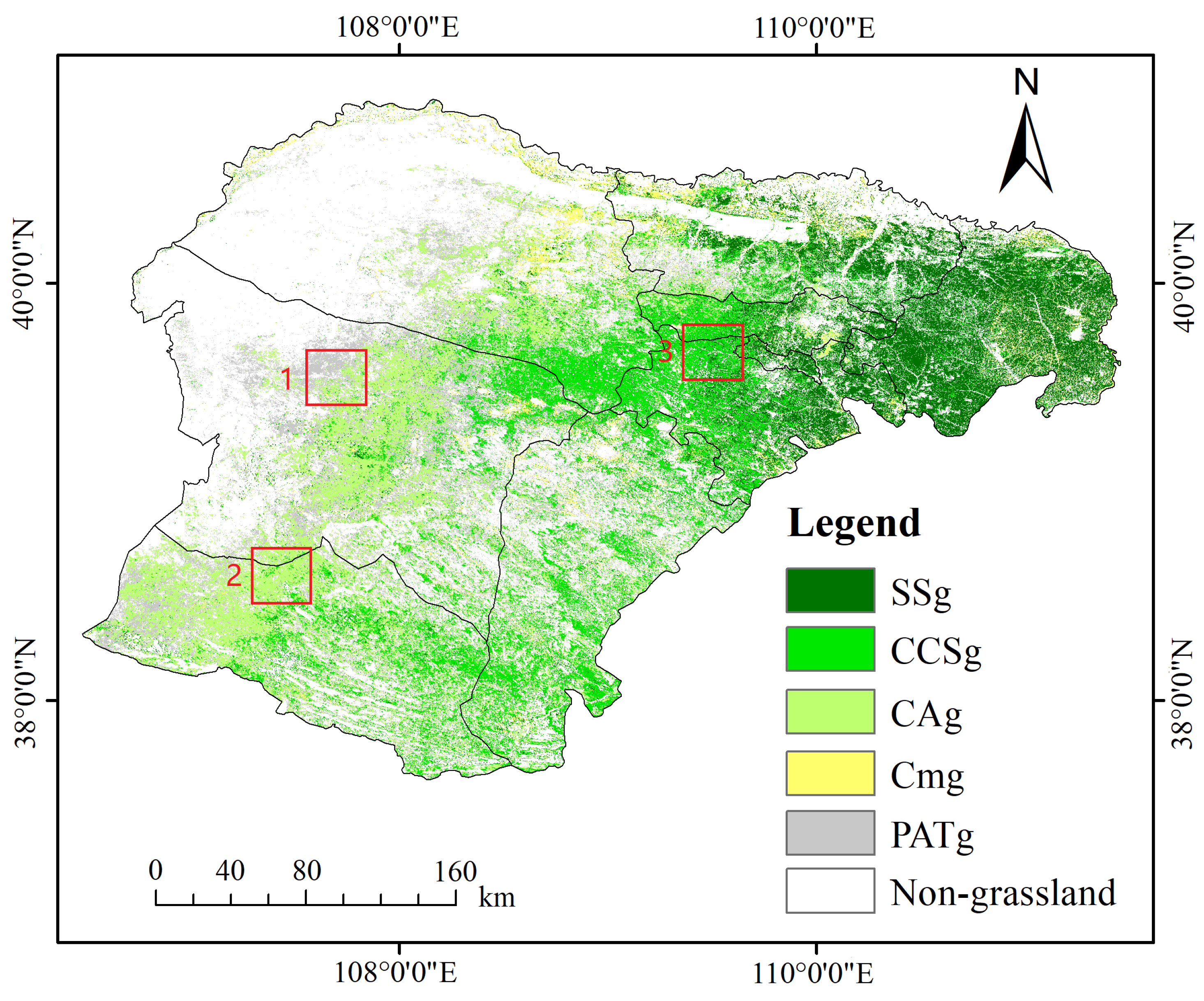
In this study, the result of Scenario 4 was applied in mapping grassland communities of Ordos (Figure 8). The corresponding confusion matrix (Table 7) reports that the overall accuracy reaches 87.25%, and the kappa coefficient reaches 0.83. The result illustrates that the 16 m GF data are reliable for differentiating grassland communities at the regional scale, integrating the EVI2 time-series and phenological features.
According to Figure 8, the distribution of the five grassland communities in the Ordos shows distinct patterns. The Caragana pumila Pojark, Caragana davazamcii Sanchir, Salix schwerinii E. L. Wolf grassland grows mainly in the central region of Ordos. The Stipa breviflora Griseb and Stipa bungeana Trin grassland is concentrated in the northeast. The Potaninia mongolica Maxim, Ammopiptanthus mongolicus S. H. Cheng, Tetraena mongolica Maxim grassland and the Caryopteris mongholica Bunge and Artemisia ordosica Krasch grassland are staggered in the southwest. The Calligonum mongolicum Turcz grassland primarily grows in the northern area.
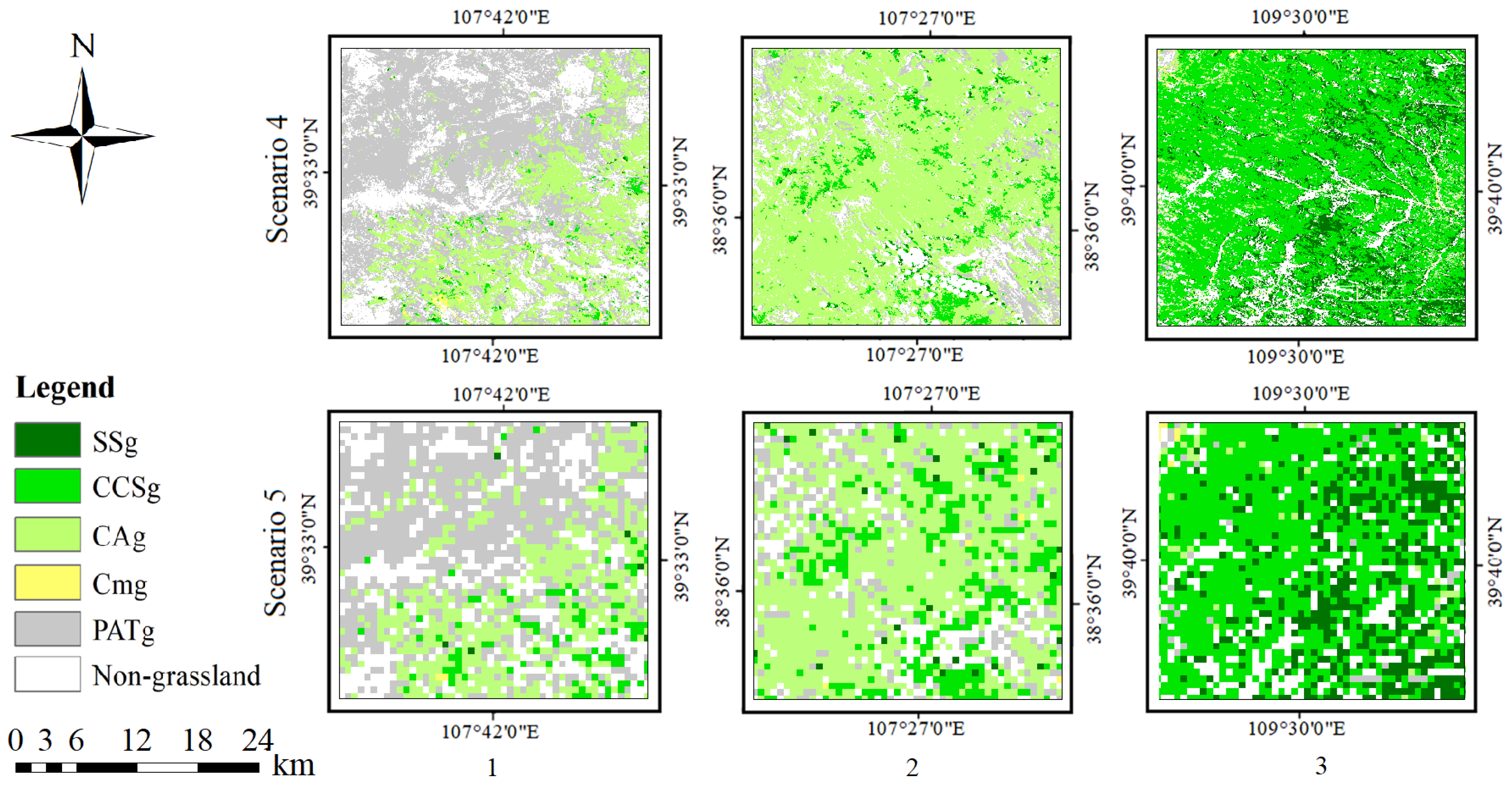
To verify the 16 m spatial resolution images’ superiority over 500 m resolution images in grassland community mapping, we selected three subdomains (marked in Figure 8) from the study area and compared the results from Scenarios 4 and 5. As shown in Figure 9, Scenario 4’s results are more detailed, and the boundaries between different communities are more clearly defined than those of Scenario 5. This result indicates that classification results based on the 16 m spatial resolution image are superior.

5. Discussion

5.1. Applicability of GF-1/6 Satellite Data in Regional-Scale Grassland Communities Classification

To improve the classification accuracy of grassland communities with satellite-borne multispectral data, the PCA EVI2 time-series data and phenological features were employed in this study. However, the acquisition of these data requires a short revisit cycle of the satellite. With the advantage of a short return period (2 d), the GF-1/6 satellite is very suitable for this task. Meanwhile, compared to most satellites with short revisit cycles, such as MODIS, the GF-1/6 satellite, with a finer spatial resolution (16 m ), can pick up more detail on the surface [32,34], thus improving the classification accuracy of grassland communities. Based on the results of Scenarios 4 and 5, under the same conditions, the classification accuracy is improved by 23.96% with GF data than that of MODIS data.
Nevertheless, it should be noted that the 16 m resolution image does contribute to the improvement in the classification accuracy of grassland communities, but also increases the volume of data, which makes the classification become time-consuming. With the construction of multiple cloud computing platforms, in future work, we will attempt to conduct the experiments on advanced remote sensing platforms such as the Google Earth Engine [67]. Relying on cloud computing’s powerful performance, we can complete the acquisition and processing of large volumes of data in a short time.

5.2. Limitation of ESTARFM Algorithm

Although the GF-1/6 satellite can provide sufficient data for this study, as with other optical satellites, the usage of GF-1/6 data is still affected by weather conditions [68]. Therefore, the ESTARFM algorithm was performed in this study and the results of fusion suggest that it is reliable to use this algorithm with the GF-1/6 WFV data. However, it is worth noting that there are still errors compared to using actual images. Moreover, the accuracy of the fusion results is affected by the effect of pre-processing, the setting of parameters in the algorithm [44], and the change in land cover types [37], which increases the uncertainty of the fusion result. With many satellite data becoming available, we will attempt to integrate multi-sensor and multi-source datasets, such as Sentinel-2 and Landsat 8, to obtain multispectral time-series data.

5.3. Grassland Classification in Ordos

Based on previous research, the vital phenological features and the time-series VI data provide additional useful information for the classification of grassland [1], because they reveal the growth characteristics of different grassland communities [28], which cannot be expressed by multispectral data. Therefore, in this study, we attempted to employ the PCA EVI2 time-series and phenological features derived from fused temporal EVI2 data in grassland community classification. We supposed that the inclusion of these features could provide a more valid basis for differentiating grassland communities and improving the accuracy of the classification.
According to the result, the classification in Scenario 1, which used only the four bands of multispectral data, yields the lowest overall accuracy and kappa coefficient. With the addition of PCA EVI2 time-series and phenological features, the classifications in Scenario 2 and Scenario 3 improve the classification accuracy by 9.63% and 14.7%, respectively. Using both of these data for classification, the accuracy of the classification in Scenario 4 is even higher (27.36%). The results indicate that compared to using multispectral data only, the method that integrates multispectral data, PCA EVI2 time-series, and phenological features contributes to improving the classification accuracy of grassland communities.
In this study, we classify the grasslands of Ordos into five communities, including the Caragana pumila Pojark, Caragana davazamcii Sanchir, Salix schwerinii E. L. Wolf grassland, the Potaninia mongolica Maxim, Ammopiptanthus mongolicus S. H. Cheng, Tetraena mongolica Maxim grassland, the Caryopteris mongholica Bunge and Artemisia ordosica Krasch grassland, the Calligonum mongolicum Turcz grassland, and the Stipa breviflora Griseb and Stipa bungeana Trin grassland, with an overall accuracy of 87.25%. Although we achieved a promising result, it should be noted that we only classified the main grassland in the study area at community level, but not at species level. Combining emerging satellite-borne hyperspectral data, such as the Orbita Hyperspectral Satellite (OHS) data, with EVI2 time-series and phenological features to achieve finer grass species classification is the focus of our future work.

6. Conclusions

This study explored regional-scale grassland classification using 23 phases of GF satellite data. The ESTARFM algorithm was validated for its applicability on GF data to generate 16 m spatial resolution cloudless time-series data. Combined with phenological features, PCA EVI2 time-series and multispectral data, the five main grassland communities of Ordos were classified with overall accuracy of 87.25%. The results reveal that the addition of either EVI2 time-series or phenological features can improve the classification accuracy of grassland communities, and the combined utilization of them is even more effective. The results also show that classification of grassland using the 16 m resolution GF data with multi-features performed much better than that using the 500 m MODIS data with the same features (overall accuracy: 87% compared to 63%), which highlights the advantage of fine spatial resolution for grassland community classification. In summary, this study proves that the proposed method can serve as a basis for the grassland community classification of large areas with moderate- and high-resolution images.

Author Contributions

Z.W. performed the experiments and wrote the manuscript. J.Z. designed the idea of the research and supervised the study. F.D. was responsible for the data analysis. G.L., D.L. and M.J. assisted in collating validation data. S.Z., D.Z., L.X., and T.J. revised this manuscript. All authors have read and agreed to the published version of the manuscript.

Funding

This research was jointly funded by the CAS Strategic Priority Research Program [Grant No. XDA19030402], the National Key Research and Development Program of China (Grant No. 2016YFD0300101), the National Natural Science Foundation of China [Grant Nos. 41871253, 42071425].

Data Availability Statement

Data available on request.

Acknowledgments

The authors want to thank Xiaolin Zhu for his help in the ESTARFM algorithm. The authors also thank Peng Gong and the University of Tsinghua for providing the land cover data in Ordos.

Conflicts of Interest

The authors declare no conflict of interest.

References

  1. Zillmann, E.; Gonzalez, A.; Herrero, E.J.M.; van Wolvelaer, J.; Esch, T.; Keil, M.; Weichelt, H.; Garzón, A.M. Pan-European grassland mapping using seasonal statistics from multisensor image time series. IEEE J. Sel. Top. Appl. Earth Obs. Remote Sens. 2014, 7, 3461–3472. [Google Scholar] [CrossRef]
  2. Xu, D. Distribution Change and Analysis of Different Grassland Types in Hulunber Grassland. Ph.D. Thesis, Chinese Academy of Agricultural Sciences Dissertation, Beijing, China, 2019. [Google Scholar]
  3. Lu, B.; He, Y. Species classification using Unmanned Aerial Vehicle (UAV)-acquired high spatial resolution imagery in a heterogeneous grassland. ISPRS J. Photogramm. Remote Sens. 2017, 128, 73–85. [Google Scholar] [CrossRef]
  4. Price, K.P.; Guo, X.; Stiles, J.M. Comparison of Landsat TM and ERS-2 SAR data for discriminating among grassland types and treatments in eastern Kansas. Comput. Electron. Agric. 2002, 37, 157–171. [Google Scholar] [CrossRef]
  5. Raab, C.; Stroh, H.G.; Tonn, B.; Meißner, M.; Rohwer, N.; Balkenhol, N.; Isselstein, J. Mapping semi-natural grassland communities using multi-temporal RapidEye remote sensing data. Int. J. Remote Sens. 2018, 39, 5638–5659. [Google Scholar] [CrossRef]
  6. Cui, X.; Guo, Z.G.; Liang, T.G.; Shen, Y.Y.; Liu, X.Y.; Liu, Y. Classification management for grassland using MODIS data: A case study in the Gannan region, China. Int. J. Remote Sens. 2012, 33, 3156–3175. [Google Scholar] [CrossRef]
  7. Yao, F.; Tang, Y.; Wang, P.; Zhang, J. Estimation of maize yield by using a process-based model and remote sensing data in the Northeast China Plain. Phys. Chem. Earth 2015, 87, 142–152. [Google Scholar] [CrossRef]
  8. Zlinszky, A.; Schroiff, A.; Kania, A.; Deák, B.; Mücke, W.; Vári, Á.; Székely, B.; Pfeifer, N. Categorizing grassland vegetation with full-waveform airborne laser scanning: A feasibility study for detecting Natura 2000 habitat types. Remote Sens. 2014, 6, 8056–8087. [Google Scholar] [CrossRef] [Green Version]
  9. Marcinkowska-Ochtyra, A.; Jarocińska, A.; Bzdęga, K.; Tokarska-Guzik, B. Classification of expansive grassland species in different growth stages based on hyperspectral and LiDAR data. Remote Sens. 2018, 10, 2019. [Google Scholar] [CrossRef] [Green Version]
  10. Melville, B.; Lucieer, A.; Aryal, J. Classification of lowland native grassland communities using hyperspectral Unmanned Aircraft System (UAS) Imagery in the Tasmanian midlands. Drones 2019, 3, 5. [Google Scholar] [CrossRef] [Green Version]
  11. Lu, B.; He, Y. Optimal spatial resolution of Unmanned Aerial Vehicle (UAV)-acquired imagery for species classification in a heterogeneous grassland ecosystem. GISci. Remote Sens. 2018, 55, 205–220. [Google Scholar] [CrossRef]
  12. Jarocińska, A.; Kopeć, D.; Tokarska-Guzik, B.; Raczko, E. Intra-Annual Variabilities of Rubus caesius L. Discrimination on Hyperspectral and LiDAR Data. Remote Sens. 2021, 13, 107. [Google Scholar] [CrossRef]
  13. Clark, M.L. Comparison of simulated hyperspectral HyspIRI and multispectral Landsat 8 and Sentinel-2 imagery for multi-seasonal, regional land-cover mapping. Remote Sens. Environ. 2017, 200, 311–325. [Google Scholar] [CrossRef]
  14. Hościło, A.; Lewandowska, A. Mapping forest type and tree species on a regional scale using multi-temporal Sentinel-2 data. Remote Sens. 2019, 11, 929. [Google Scholar] [CrossRef] [Green Version]
  15. Ochtyra, A.; Marcinkowska-Ochtyra, A.; Raczko, E. Threshold-and trend-based vegetation change monitoring algorithm based on the inter-annual multi-temporal normalized difference moisture index series: A case study of the Tatra Mountains. Remote Sens. Environ. 2020, 249, 112026. [Google Scholar] [CrossRef]
  16. Hong, G.; Zhang, A.; Zhou, F.; Brisco, B. Integration of optical and synthetic aperture radar (SAR) images to differentiate grassland and alfalfa in Prairie area. Int. J. Appl. Earth Obs. Geoinf. 2014, 28, 12–19. [Google Scholar] [CrossRef]
  17. Ouyang, W.; Hao, F.; Skidmore, A.K.; Groen, T.A.; Toxopeus, A.G.; Wang, T. Integration of multi-sensor data to assess grassland dynamics in a Yellow River sub-watershed. Ecol. India. 2012, 18, 163–170. [Google Scholar] [CrossRef]
  18. Hill, M.J. Vegetation index suites as indicators of vegetation state in grassland and savanna: An analysis with simulated SENTINEL 2 data for a North American transect. Remote Sens. Environ. 2013, 137, 94–111. [Google Scholar] [CrossRef]
  19. Yang, L.; Jin, S.; Danielson, P.; Homer, C.; Gass, L.; Bender, S.M.; Casei, A.; Costellog, C.; Dewitzd, J.; Fryc, J.; et al. A new generation of the United States National Land Cover Database: Requirements, research priorities, design, and implementation strategies. ISPRS J. Photogramm. Remote Sens. 2018, 146, 108–123. [Google Scholar] [CrossRef]
  20. McInnes, W.S.; Smith, B.; McDermid, G.J. Discriminating native and nonnative grasses in the dry mixedgrass prairie with MODIS NDVI time series. IEEE J. Sel. Top. Appl. Earth Obs. Remote Sens. 2015, 8, 1395–1403. [Google Scholar] [CrossRef]
  21. Rapinel, S.; Mony, C.; Lecoq, L.; Clement, B.; Thomas, A.; Hubert-Moy, L. Evaluation of Sentinel-2 time-series for mapping floodplain grassland plant communities. Remote Sens. Environ. 2019, 223, 115–129. [Google Scholar] [CrossRef]
  22. Wen, Q.; Zhang, Z.; Liu, S.; Wang, X.; Wang, C. Classification of grassland types by MODIS time-series images in Tibet, China. IEEE J. Sel. Top. Appl. Earth Obs. Remote Sens. 2010, 3, 404–409. [Google Scholar] [CrossRef]
  23. Schuster, C.; Schmidt, T.; Conrad, C.; Kleinschmit, B.; Förster, M. Grassland habitat mapping by intra-annual time series analysis—Comparison of RapidEye and TerraSAR-X satellite data. Int. J. Appl. Earth Obs. Geoinf. 2015, 34, 25–34. [Google Scholar] [CrossRef]
  24. Franke, J.; Keuck, V.; Siegert, F. Assessment of grassland use intensity by remote sensing to support conservation schemes. J. Nat. Conserv. 2012, 20, 125–134. [Google Scholar] [CrossRef]
  25. Shi-Bo, F.; Xin-Shi, Z. Control of vegetation distribution: Climate, geological substrate, and geomorphic factors. A case study of grassland in Ordos, Inner Mongolia, China. Can. J. Remote Sens. 2013, 39, 167–174. [Google Scholar] [CrossRef]
  26. Schmidt, T.; Schuster, C.; Kleinschmit, B.; Förster, M. Evaluating an intra-annual time series for grassland classification—How many acquisitions and what seasonal origin are optimal? IEEE J. Sel. Top. Appl. Earth Obs. Remote Sens. 2014, 7, 3428–3439. [Google Scholar] [CrossRef]
  27. Park, D.S.; Breckheimer, I.; Williams, A.C.; Law, E.; Ellison, A.M.; Davis, C.C. Herbarium specimens reveal substantial and unexpected variation in phenological sensitivity across the eastern United States. Phil. Trans. R. Soc. B 2019, 374, 20170394. [Google Scholar] [CrossRef] [PubMed]
  28. Wang, C.; Long, R.; Ding, L. The effects of differences in functional group diversity and composition on plant community productivity in four types of alpine meadow communities. Biodivers. Sci. 2004, 12, 403–409. [Google Scholar]
  29. Wang, C.; Guo, H.; Zhang, L.; Qiu, Y.; Sun, Z.; Liao, J.; Liu, G.; Zhang, Y. Improved alpine grassland mapping in the Tibetan Plateau with MODIS time series: A phenology perspective. Int. J. Digit. Earth 2015, 8, 133–152. [Google Scholar] [CrossRef]
  30. Yoo, C.; Im, J.; Park, S.; Quackenbush, L.J. Estimation of daily maximum and minimum air temperatures in urban landscapes using MODIS time series satellite data. ISPRS J. Photogramm. Remote Sens. 2018, 137, 149–162. [Google Scholar] [CrossRef]
  31. Zhou, J.; Jia, L.; Menenti, M. Reconstruction of global MODIS NDVI time series: Performance of Harmonic ANalysis of Time Series (HANTS). Remote Sens. Environ. 2015, 163, 217–228. [Google Scholar] [CrossRef]
  32. Yang, X.; Yang, T.; Ji, Q.; He, Y.; Ghebrezgabher, M.G. Regional-scale grassland classification using moderate-resolution imaging spectrometer datasets based on multistep unsupervised classification and indices suitability analysis. J. Appl. Remote Sens. 2014, 8, 083548. [Google Scholar] [CrossRef]
  33. Xu, K.; Tian, Q.; Yang, Y.; Yue, J.; Tang, S. How up-scaling of remote-sensing images affects land-cover classification by comparison with multiscale satellite images. J. Appl. Remote Sens. 2019, 40, 2784–2810. [Google Scholar] [CrossRef]
  34. Zheng, L. Crop Classification Using Multi-Features of Chinese Gaofen-1/6 Sateliite Remote Sensing Images. Ph.D. Thesis, University of Chinese Academy of Sciences, Beijing, China, 2019. [Google Scholar]
  35. Kong, F.; Li, X.; Wang, H.; Xie, D.; Li, X.; Bai, Y. Land cover classification based on fused data from GF-1 and MODIS NDVI time series. Remote Sens. 2016, 8, 741. [Google Scholar] [CrossRef] [Green Version]
  36. Jin, S.; Homer, C.; Yang, L.; Xian, G.; Fry, J.; Danielson, P.; Townsend, P.A. Automated cloud and shadow detection and filling using two-date Landsat imagery in the USA. Int. J. Remote Sens. 2013, 34, 1540–1560. [Google Scholar] [CrossRef]
  37. Zhang, H.K.; Huang, B. A new look at image fusion methods from a Bayesian perspective. Remote Sens. 2015, 7, 6828–6861. [Google Scholar] [CrossRef] [Green Version]
  38. Tao, G.; Jia, K.; Zhao, X.; Wei, X.; Xie, X.; Zhang, X.; Wang, B.; Yao, Y.; Zhang, X. Generating High Spatio-Temporal Resolution Fractional Vegetation Cover by Fusing GF-1 WFV and MODIS Data. Remote Sens. 2019, 11, 2324. [Google Scholar] [CrossRef] [Green Version]
  39. Yang, G.; Weng, Q.; Pu, R.; Gao, F.; Sun, C.; Li, H.; Zhao, C. Evaluation of ASTER-like daily land surface temperature by fusing ASTER and MODIS data during the HiWATER-MUSOEXE. Remote Sens. 2016, 8, 75. [Google Scholar] [CrossRef] [Green Version]
  40. Tewes, A.; Thonfeld, F.; Schmidt, M.; Oomen, R.J.; Zhu, X.; Dubovyk, O.; Menz, G.; Schellberg, J. Using RapidEye and MODIS data fusion to monitor vegetation dynamics in semi-arid rangelands in South Africa. Remote Sens. 2015, 7, 6510–6534. [Google Scholar] [CrossRef] [Green Version]
  41. Zhou, X.; Wang, P.; Tansey, K.; Zhang, S.; Li, H.; Wang, L. Developing a fused vegetation temperature condition index for drought monitoring at field scales using Sentinel-2 and MODIS imagery. Comput. Electron. Agric. 2020, 168, 105144. [Google Scholar] [CrossRef]
  42. Wu, M.; Huang, W.; Niu, Z.; Wang, C. Combining HJ CCD, GF-1 WFV and MODIS data to generate daily high spatial resolution synthetic data for environmental process monitoring. Int. J. Environ. Res. Public Health 2015, 12, 9920–9937. [Google Scholar] [CrossRef] [PubMed] [Green Version]
  43. Gao, F.; Masek, J.; Schwaller, M.; Hall, F. On the blending of the Landsat and MODIS surface reflectance: Predicting daily Landsat surface reflectance. IEEE Trans. Geosci. Remote Sens. 2006, 44, 2207–2218. [Google Scholar]
  44. Zhu, X.; Chen, J.; Gao, F.; Chen, X.; Masek, J.G. An enhanced spatial and temporal adaptive reflectance fusion model for complex heterogeneous regions. Remote Sens. Environ. 2010, 114, 2610–2623. [Google Scholar] [CrossRef]
  45. Zhang, H. Evalution on Sustainable Development of Animal Husbandry in Erdos City. Master’s Thesis, Inner Mongolia University, Hohhot, China, 2010. [Google Scholar]
  46. Jiang, Z.; Huete, A.R.; Didan, K.; Miura, T. Development of a two-band enhanced vegetation index without a blue band. Remote Sens. Environ. 2008, 112, 3833–3845. [Google Scholar] [CrossRef]
  47. Gong, P.; Liu, H.; Zhang, M.; Li, C.; Wang, J.; Huang, H.; Clinton, N.; Ji, L.; Li, W.; Bai, Y.; et al. Stable classification with limited sample: Transferring a 30-m resolution sample set collected in 2015 to mapping 10-m resolution global land cover in 2017. Sci. Bull. 2019, 64, 370–373. [Google Scholar] [CrossRef] [Green Version]
  48. Liu, G. Inner Mongolia Region. In Atlas of Physical Geography of China; China Map Press: Beijing, China, 2010; pp. 171–172. [Google Scholar]
  49. Zhang, X. Scrub, Desert, and Steppe. In Vegetation and Its Geographical Pattern in China: An Illustration of the Vegetation Map of the People’s Republic of China (1:1000000); Geological Publishing House: Beijing, China, 2007; pp. 257–385. [Google Scholar]
  50. Jia, K.; Liang, S.; Gu, X.; Baret, F.; Wei, X.; Wang, X.; Yao, Y.; Yang, L.; Li, Y. Fractional vegetation cover estimation algorithm for Chinese GF-1 wide field view data. Remote Sens. Environ. 2016, 177, 184–191. [Google Scholar] [CrossRef]
  51. Yang, A.; Zhong, B.; Hu, L.; Wu, S.; Xu, Z.; Wu, H.; Wu, J.; Gong, X.; Wang, H.; Liu, Q. Radiometric Cross-Calibration of the Wide Field View Camera Onboard GaoFen-6 in Multispectral Bands. Remote Sens. 2020, 12, 1037. [Google Scholar] [CrossRef] [Green Version]
  52. Dobreva, I.D.; Klein, A.G. Fractional snow cover mapping through artificial neural network analysis of MODIS surface reflectance. Remote Sens. Environ. 2012, 115, 3355–3366. [Google Scholar] [CrossRef] [Green Version]
  53. Xun, L.; Zhang, J.; Cao, D.; Zhang, S.; Yao, F. Crop Area Identification Based on Time Series EVI2 and Sparse Representation Approach: A Case Study in Shandong Province, China. IEEE Access 2019, 7, 157513–157523. [Google Scholar] [CrossRef]
  54. Savitzky, A.; Golay, M.J. Smoothing and differentiation of data by simplified least squares procedures. Anal. Chem. 1964, 36, 1627–1639. [Google Scholar] [CrossRef]
  55. Chen, J.; Jönsson, P.; Tamura, M.; Gu, Z.; Matsushita, B.; Eklundh, L. A simple method for reconstructing a high-quality NDVI time-series data set based on the Savitzky–Golay filter. Remote Sens. Environ. 2004, 91, 332–344. [Google Scholar] [CrossRef]
  56. Reed, B.C.; Schwartz, M.D.; Xiao, X. Remote sensing phenology. In Phenology of Ecosystem Processes; Noormets, A., Ed.; Springer: New York, NY, USA, 2009; pp. 231–246. [Google Scholar]
  57. Ren, J.; Zabalza, J.; Marshall, S.; Zheng, J. Effective feature extraction and data reduction in remote sensing using hyperspectral imaging [applications corner]. IEEE Signal Process. Mag. 2014, 31, 149–154. [Google Scholar] [CrossRef] [Green Version]
  58. Zhong, L.; Hu, L.; Zhou, H. Deep learning based multi-temporal crop classification. Remote Sens. Environ. 2019, 221, 430–443. [Google Scholar] [CrossRef]
  59. Kabir, S.; Islam, R.U.; Hossain, M.S.; Andersson, K. An integrated approach of belief rule base and deep learning to predict air pollution. Sensors 2020, 20, 1956. [Google Scholar] [CrossRef] [PubMed] [Green Version]
  60. Su, P.; Li, G.; Wu, C.; Vijay-Shanker, K. Using distant supervision to augment manually annotated data for relation extraction. PLoS ONE 2019, 14, e0216913. [Google Scholar] [CrossRef] [PubMed] [Green Version]
  61. Xiong, Z.; Yu, Q.; Sun, T.; Chen, W.; Wu, Y.; Yin, J. Super-resolution reconstruction of real infrared images acquired with unmanned aerial vehicle. PLoS ONE 2020, 15, e0234775. [Google Scholar] [CrossRef]
  62. Lopatin, J.; Fassnacht, F.E.; Kattenborn, T.; Schmidtlein, S. Mapping plant species in mixed grassland communities using close range imaging spectroscopy. Remote Sens. Environ. 2017, 201, 12–23. [Google Scholar] [CrossRef]
  63. Tan, C.; Zhang, P.; Zhang, Y.; Zhou, X.; Wang, Z.; Du, Y.; Mao, W.; Li, W.; Wang, D.; Guo, W. Rapid Recognition of Field-Grown Wheat Spikes Based on a Superpixel Segmentation Algorithm Using Digital Images. Front. Plant Sci. 2020, 11, 259. [Google Scholar] [CrossRef] [Green Version]
  64. Maulik, U.; Chakraborty, D. Remote sensing image classification: A survey of support-vector-machine-based advanced techniques. IEEE Geosci. Remote Sens. Mag. 2017, 5, 33–52. [Google Scholar] [CrossRef]
  65. Mountrakis, G.; Im, J.; Ogole, C. Support vector machines in remote sensing: A review. ISPRS J. Photogramm. Remote Sens. 2011, 66, 247–259. [Google Scholar] [CrossRef]
  66. Hao, P.; Wang, L.; Niu, Z.; Aablikim, A.; Huang, N.; Xu, S.; Chen, F. The potential of time series merged from Landsat-5 TM and HJ-1 CCD for crop classification: A case study for Bole and Manas Counties in Xinjiang, China. Remote Sens. 2014, 6, 7610–7631. [Google Scholar] [CrossRef] [Green Version]
  67. Gorelick, N.; Hancher, M.; Dixon, M.; Ilyushchenko, S.; Thau, D.; Moore, R. Google Earth Engine: Planetary-scale geospatial analysis for everyone. Remote Sens. 2017, 202, 18–27. [Google Scholar] [CrossRef]
  68. Dusseux, P.; Corpetti, T.; Hubert-Moy, L.; Corgne, S. Combined use of multi-temporal optical and radar satellite images for grassland monitoring. Remote Sens. 2014, 6, 6163–6182. [Google Scholar] [CrossRef] [Green Version]
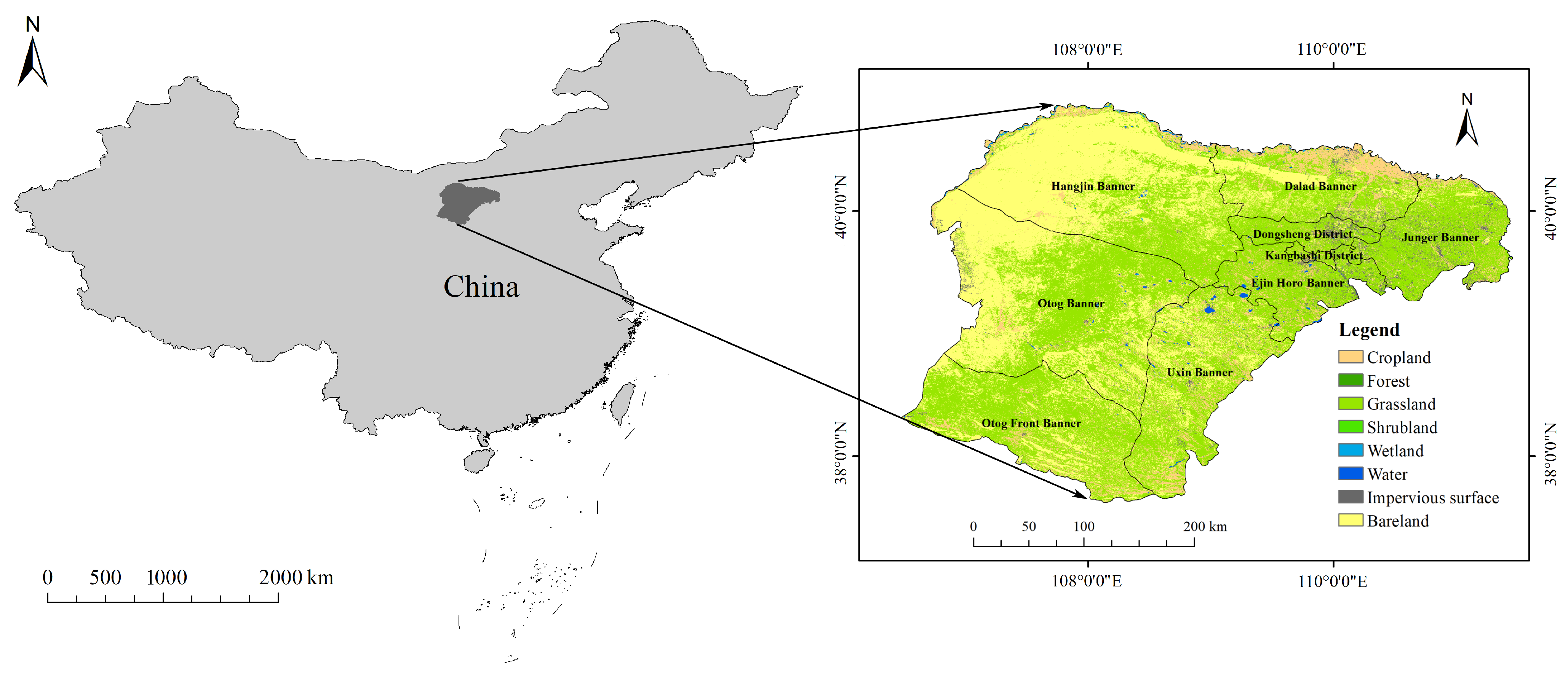
Figure 1. The location and land cover of Ordos [47].
Remotesensing 13 00835 g001
Figure 2. The flowchart of the grassland community classification in Ordos.
Remotesensing 13 00835 g002
Figure 3. The flowchart of the Enhanced Spatial and Temporal Adaptive Reflectance Fusion Model (ESTARFM) algorithm.
Remotesensing 13 00835 g003
Figure 4. An example showing the smoothing effect of EVI2 time-series under different parameters of S–G filter (one pixel in grassland): (a) q = 2, r = 4, 5, 6 respectively. (b) r = 5, q = 1, 2, 3 respectively.
Remotesensing 13 00835 g004
Figure 5. Comparisons of the fused EVI2 data with the corresponding the actual GF EVI2 images.
Remotesensing 13 00835 g005
Figure 6. Representative scatter plots between actual EVI2 and fused EVI2, and residuals histogram of Region A, B and C.
Remotesensing 13 00835 g006
Figure 7. Two examples of de-clouding based on the ESTARFM algorithm.
Remotesensing 13 00835 g007
Figure 8. The mapping of grassland communities in Ordos for Scenario 4.
Remotesensing 13 00835 g008
Figure 9. The mapping grassland communities of three subdomains to compare Scenarios 4 and 5.
Remotesensing 13 00835 g009
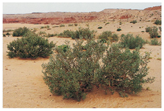
Table 1. The five main grassland communities in Ordos.
Dominant Species [48]Total Coverage (%) [49]Examples
CCSgCaragana pumila Pojark,
Caragana davazamcii Sanchir,
Salix schwerinii E. L. Wolf
20–30 Remotesensing 13 00835 i001
PATgPotaninia mongolica Maxim,
Ammopiptanthus mongolicus S. H. Cheng,
Tetraena mongolica Maxim
10–20 Remotesensing 13 00835 i002
CAgCaryopteris mongholica Bunge,
Artemisia ordosica Krasch
2–6 Remotesensing 13 00835 i003
CmgCalligonum mongolicum Turcz5–10 Remotesensing 13 00835 i004
SSgStipa breviflora Griseb,
Stipa bungeana Trin
30–45 Remotesensing 13 00835 i005
Table 2. The band information of GF-1 and GF-6 satellites.
BandGF-1GF-6Wavelength ( μ m)
1BlueBlue0.45–0.52
2GreenGreen0.52–0.59
3RedRed0.63–0.69
4NIRNIR0.77–0.89
5 Red-edge 10.69–0.73
6 Red-edge 20.73–0.77
7 Yellow edge0.40–0.45
8 Purple edge0.59–0.63
Table 3. The main properties of the GF-1 and GF-6 data used in this study.
SatelliteAcquisition TimeCloud PercentageNumber of Images
GF-113 December 2018Less than 1%7
GF-12 January 20192%6
GF-612 January 2019No cloud2
GF-14 February 2019No cloud7
GF-622 February 20195%2
GF-69 March 20191%3
GF-622 March 2019No cloud2
GF-64 April 20198%3
GF-625 April 20194%2
GF-113 May 20193%8
GF-122 May 2019No Cloud7
GF-69 June 201910%2
GF-1, GF-629 June 2019,
1 July 2019
7%6
GF-114 July 20199%4
GF-61 August 20192%2
GF-115 August 20199%6
GF-1, GF-628 August 2019,
30 August 2019
2%3
GF-1, GF-614 September 2019,
15 September 2019
15%3
GF-1, GF-627 September 2019,
30 September 2019
1%4
GF-618 October 20195%2
GF-630 October 2019No Cloud2
GF-114 November 20191%7
GF-1, GF-66 December 2019,
8 December 2019
1%4
Table 4. Number of pixels in each grassland community used for training and validating the SVM classification.
CCSgPATgCAgCmgSSg
Samples used for SVM training
Number of pixels98784230713816879770
Samples used for SVM testing
Number of pixels2320106317144322654
Table 5. The values of the six phenological features for the five grassland communities.
Maximum EVI2Minimum EVI2Mean EVI2Phenology IndexStart of Season
(Days)
End of Season
(Days)
CCSg0.5260.0890.2710.112104297
PATg0.3330.0610.1810.07590278
CAg0.3610.0750.2030.083106306
Cmg0.4790.0220.2370.122100299
SSg0.6380.0470.3020.136109298
Table 6. Accuracy assessment and comparison of different scenarios.
ScenarioInput DataOverall Acc. (%)Kappa Coefficient
1GF multispectral data59.890.4577
2GF multispectral data and PCA EVI2 time-series69.520.5953
3GF multispectral data and phenological features74.590.6612
4GF multispectral data, PCA EVI2 time-series
and phenological feature
87.250.8309
5MODIS multispectral data, PCA EVI2 time-series
and phenological feature
63.290.5314
Table 7. The confusion matrix and accuracy assessment of Scenario 4.
Reference Data (Pixels)Prod. Acc. (%)User Acc. (%)
Class (pixels)CCSgPATgCAgCmgSSgTotal
CCSg20091710270235186.5985.45
PATg1583010236098378.0884.44
CAg82232153801185389.7383.00
Cmg94033961650991.6777.80
SSg1200002367248789.1995.17
Total2320106317144322654
Overall accuracy = 87.25%, kappa coefficient = 0.83.
Publisher’s Note: MDPI stays neutral with regard to jurisdictional claims in published maps and institutional affiliations.