Article

Using Saildrones to Validate Arctic Sea-Surface Salinity from the SMAP Satellite and from Ocean Models

1
Jet Propulsion Laboratory, California Institute of Technology, Pasadena, CA 91109, USA
2
Farallon Institute, Petaluma, CA 94952, USA
3
Moss Landing Marine Laboratories, San José State University, Moss Landing, CA 95039, USA
4
Physical Oceanography Department, Center for Scientific Research and Higher Education at Ensenada, Ensenada 22860, Mexico
5
Institute of Oceanography, University of Sao Paolo, São Paulo 05508-120, Brazil
6
Polar Science Center, Applied Physics Lab, University of Washington, Seattle, WA 98105, USA
*
Author to whom correspondence should be addressed.
Remote Sens. 2021, 13(5), 831; https://doi.org/10.3390/rs13050831
Submission received: 15 January 2021 / Revised: 18 February 2021 / Accepted: 20 February 2021 / Published: 24 February 2021
(This article belongs to the Special Issue Remote Sensing of the Polar Oceans)

Abstract

:
The Arctic Ocean is one of the most important and challenging regions to observe—it experiences the largest changes from climate warming, and at the same time is one of the most difficult to sample because of sea ice and extreme cold temperatures. Two NASA-sponsored deployments of the Saildrone vehicle provided a unique opportunity for validating sea-surface salinity (SSS) derived from three separate products that use data from the Soil Moisture Active Passive (SMAP) satellite. To examine possible issues in resolving mesoscale-to-submesoscale variability, comparisons were also made with two versions of the Estimating the Circulation and Climate of the Ocean (ECCO) model (Carroll, D; Menmenlis, D; Zhang, H.). The results indicate that the three SMAP products resolve the runoff signal associated with the Yukon River, with high correlation between SMAP products and Saildrone SSS. Spectral slopes, overall, replicate the −2.0 slopes associated with mesoscale-submesoscale variability. Statistically significant spatial coherences exist for all products, with peaks close to 100 km. Based on these encouraging results, future research should focus on improving derivations of satellite-derived SSS in the Arctic Ocean and integrating model results to complement remote sensing observations.

Graphical Abstract

1. Introduction

The Arctic is one of the most critical areas for both climate and biodiversity [1,2]. Yet, it is also one of the most under sampled, due to the difficulty of environmental conditions and seasonality of sea-ice cover. The western coast of Alaska contains one of the world’s most productive fisheries, which are influenced by seasonal stratification and interannual variability in Chlorophyll-a [1,3,4]. One example is the Yukon River estuary, where changes in stratification are governed by river runoff, sea-ice melt, and precipitation. The mouth of the river is located at 62°35′55″N 164°48′00″W and empties into the Bering Sea at the Yukon–Kuskokwim (Y-K) Delta. The Y-K Delta is a substantial source of terrestrial freshwater, which can drive large gradients and temporal variability in sea-surface salinity (SSS). Thus, part of this paper’s focus is to examine how well SMAP and model-derived SSS can detect the low-SSS signal from the Y-K Delta shelf, where low- salinity water exits from the Yukon and other rivers, with secondary inputs from sea-ice melt and net precipitation minus evaporation. Our analysis should be taken as a preliminary step in the comparison of observations and models to encourage future research and applications in this region.
During spring to summer 2019, six deployments of the Saildrone vehicle were conducted off Alaska’s west and northwestern coastline: four funded by NOAA and two by NASA. This paper will focus on the two NASA deployments, SD1036 and SD1037 (see Figure 1). Both were launched from Dutch Harbor on 14 May 2019, and recovered on 11 October 2019.
Remote sensing from satellites provides a unique opportunity to monitor this critical region, but in-situ validation studies also need to be conducted to assess the accuracy of satellite observations. Recent studies by [5,6] suggest that sea-surface salinity from NASA’s Soil Moisture Active Passive Mission and ESA’s Soil Moisture Ocean Salinity Mission agree well in terms of the annual-mean signal. They also found better agreement further from the Marginal Ice Zone in warmer waters, consistent with decreasing L-Band sensitivity to salinity in colder waters. Results from [7] showed how sea level data from Jason-2 was applied to derive water surface height and slope dynamics associated with the Y-K delta.
Here, we build on those results to compare the capability of the SMAP SSS products, model products, and Saildrone to resolve known features associated with salinity gradients in the Bering, Chukchi, and Beaufort Seas. In the process, our goal is to quantify Saildrone-satellite-model comparisons to provide information for future applications in this challenging but critical region of the world’s oceans.
Comparisons are also shown for the spectra derived from the Saildrone. These comparisons reveal possible differences in the different data sets’ resolvability, which depends on spatial resolution and smoothing. These types of comparisons were used in [8]. Spectral slopes were consistent with the mesoscale and submesoscale variability associated in the California Current System. In addition to spectra, coherences are also examined to determine possible relationships in the wavenumber spectra between the different products and the Saildrone-derived SSS.
The objectives of this paper are:
(1)
Validation and comparison of SMAP salinity products in the Arctic Ocean.
(2)
Comparisons with low- and high-resolution numerical ocean models to determine if high-resolution models are indicative of spatial variability that is not resolved by remote sensing products.

2. Material and Methods

2.1. Data

2.1.1. Satellite Salinity Data

Three different SMAP SSS data sets were used in the study, all using Level 3 8-day running means. These include the Jet Propulsion Laboratory Cap Active Passive Version 4.3 (JPLSSS) (https://doi.org/10.5067/SMP43-3TPCS, data set and the Remote Sensing Systems Version 4.0 40 km (RSS40km) (https://doi.org/10.5067/SMP40-3SPCS) and 70 km (RSS70km) data sets. Data can be retrieved from the Physical Oceanography Distributed Active Archive Center (PO. DAAC) at https://podaac.jpl.nasa.gov. All data sets were accessed on 1 June 2020. All products are distributed in a 0.25° rectangular projection, where the gridding is not indicative of the product’s spatial resolution. The JPLSSS has an inherent feature resolution of 60 km. The RSS40km has a 40 km feature resolution, and the RSS70km has a 70 km feature resolution. The RSS70km product is created by smoothing the RSS40km product. Brief descriptions of data product characteristics are given below.
The JPLSSS v4.3 derives SSS from SMAP data using a JPL-developed algorithm. This version has an improved land correction, which is useful for our coastal analysis [9]. The RSS v4.0 SSS products include an improved land correction and sea-ice mask, and consolidation of both 40-km and 70-km SMAP-SSS datasets as variable fields in a single data product [10]. These two products are derived from the same SMAP brightness temperatures, but use a methodology different from JPLSSS to connect brightness temperatures to ocean salinity values.

2.1.2. In-Situ Saildrone Measurements

Saildrones SD1036 and SD1037 were deployed from 15 May 2019, through 11 October 2019. Leaving from Dutch Harbor, AK, the vehicles headed north through the Bering Strait and continued into the Chukchi Sea. Both deployments were carried out simultaneously, but did not necessarily follow identical tracks. As the Arctic Ocean sea ice melted, the vehicles explored the Beaufort Sea until decreasing light (Saildrones are solar powered) forced them to retreat southward and return to Dutch Harbor. The vehicles had the standard assortment of instruments onboard, including a Seabird 37 Conductivity, Temperature, Depth (CTD) and RBR 040805 CTD, IR pyrometer, fluorometer, dissolved oxygen sensor, anemometer, barometer, and Acoustic Doppler Current Profiler (ADCP). All data, except the ADCP, was collected continuously at one-minute intervals. Additionally, four RBR temperature data loggers were also installed along the keel. The data for this cruise is distributed through the PO. DAAC (https://podaac.jpl.nasa.gov/dataset/SAILDRONE_ARCTIC?ids=&values=&search=Saildrone). Details and characteristics of the Arctic deployment may be found at the above. For more details on the Saildrone vehicle, and validation results, please see [11]. Salinity measurements were taken at a depth of ~0.5 m.
Differences in SSS between the Seabird and RBR-derived CTD measurements were minor for SD1036, but larger differences were seen for SD1037. Based on the large spikes in the Seabird-derived salinity for the SD1037 deployment, it was decided to use the RBR data for all the comparisons. Differences between the Seabird- and RBR-derived SSS may be found in Supplementary Materials associated with this manuscript.

2.1.3. ECCO Numerical Ocean Model

The ECCO LLC270 global-ocean and sea-ice data synthesis [12] builds upon two previous ECCO efforts, ECCO v4 [13] and ECCO2 [14,15]. Compared to the lower-resolution ECCO v4 synthesis (nominal 1° grid spacing), ECCO LLC270 has finer horizontal grid spacing (~37 km at the equator and ~18 km at high latitudes). Terrestrial runoff along coastal boundaries is forced using the monthly climatology of [16]. Since the horizontal resolution of the model is insufficient to resolve mesoscale eddies, their impact on the large-scale ocean circulation is parameterized [17,18]. Remotely-sensed data constraints on the model include daily along-track sea level anomalies from satellite altimetry [19] relative to a mean dynamic topography [20], monthly ocean bottom pressure anomalies from the Gravity Recovery and Climate Experiment (GRACE) mission [21], daily mean sea surface temperature (SST) [22], and sea-ice concentration fields from passive microwave radiometry [23]. The primary in-situ data constraints include the global array of Argo floats [24,25], ship-based hydrography incorporated as monthly climatological temperature and salinity profiles from the World Ocean Atlas 2009 [26,27], tagged marine mammals [28,29], and ice-tethered profilers in the Arctic [30]. To fit the above observations, the ECCO LLC270 solution minimizes a weighted quadratic sum of model-data differences. This is done using the adjoint method, aka 4D-Var [31,32]. The control variables include initial (at the start of the model run) temperature and salinity fields; time-invariant diapycnal, isopycnal [17], and thickness diffusivities [18]; and 14-day adjustments to the 6-hourly ERA Interim [33] estimates of downward shortwave and longwave radiation, precipitation, 2-m air temperature and specific humidity, and 10-m zonal and meridional wind.
We also use LLC4320, which is similar to LLC270 but has increased spatial resolution. Briefly, the spatial resolution ranges from 0.75 km at the high latitudes to 2.2 km at the Equator. A major difference relevant to this study is that LLC4320 also includes tidal forcing. This allows for successful reproduction of shelf-slope dynamics, water mass modification, and their contribution to global-ocean circulation. Near-surface salinity data from buoys and other in-situ observations is assimilated into LLC270 within its shallowest grid cell of thickness 10 m. LLC 4320 has an uppermost grid cell thickness of 1 m and no assimilation; however, the coarser resolution simulations that provide the initial conditions are data constrained.

2.2. Collocation Method
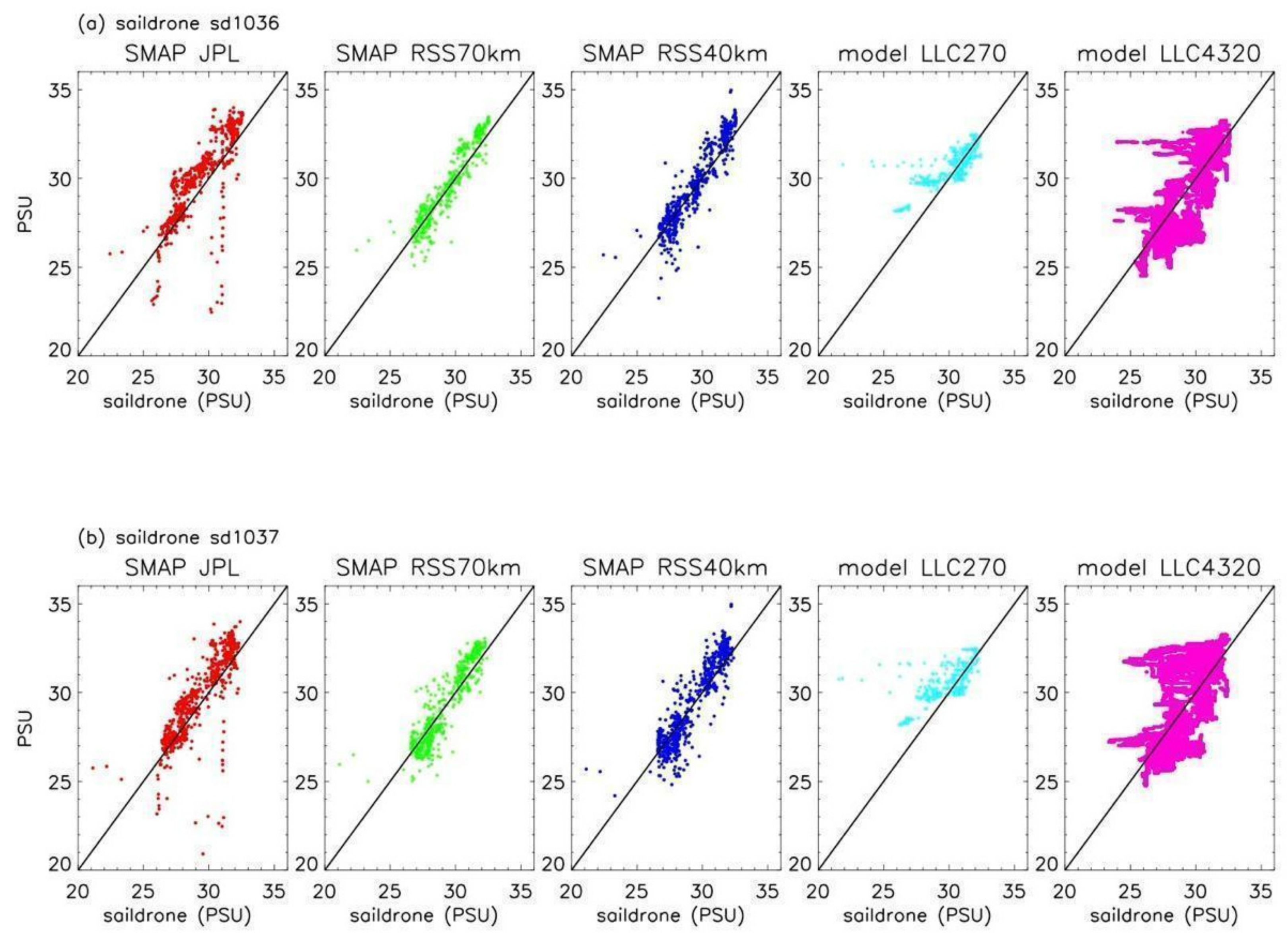
To collocate the eight-day gridded satellite data with cruise trajectory data, we used the open-source software library Xarray [34]. Xarray provides flexible interpolation routines and support for NetCDF files. We used nearest-neighbor interpolation to first match each one-minute Saildrone measurements with the gridded data. For each unique gridded satellite data point, all Saildrone data was averaged within that grid cell, providing a single matchup Saildrone data point for each single satellite retrieval. The same collocation methodology was also applied to LLC270 and LLC4320 models. Thus, all Saildrone and model data have been bin-averaged into the satellite grids. For the SMAP data, being on the same 0.25° grid, the Saildrone matchups will be identical. However, differences because of missing data due to processing differences in quality flagging may still exist. The same methodology was applied to the models, but of course will consist of different matchups due to the differences in gridding and spatial resolution.

3. Results

3.1. Saildrone Tracks SMAP/Model SSS

Figure 1 shows the spatial location of the two Saildrone deployments, overlaid on the three satellite and two model SSS products i.e., JPLSSS, RSS40km, RSS70km, LLC270, and LLC4320. Maps of SSS are time means of the SSS over the Saildrone deployment period.
Clearly visible in all the SSS maps are locations of freshening near the coast (Figure 1). Overall, the largest freshening event is observed at approximately day 150 of year 2019 and is associated with the Y-K delta discharge (also see Figure 2 and Figure 3). The magnitude of the freshening depends on the SMAP product; with regard to the models, the LLC270 shows little or no freshening, while the higher resolution LLC4320 shows similar freshening as the SMAP products. Freshening is seen at other locations along the deployment, with possible explanations including sea-ice melt, net precipitation minus evaporation, and dynamics associated with coastal and shelf currents.
All SMAP products and models show freshening located at approximately 62°N, the location of the Yukon River discharge. White colors indicate missing data due to land contamination. Missing data close to the coast is different for each of the SMAP products. Among the three SMAP products, JPLSSS (Figure 1a) provides data closest to the land, which is an indication of the robustness of land correction implemented in JPL algorithm; while the smoothing procedures of RSS algorithm results in RSS70km (Figure 1b) having larger gaps near the coast compared to RSS40km (Figure 1c). It is important to note that although the JPLSSS provides data closer to land, Root Mean Square Differences (RMSD), as defined between the product and Saildrone (see Table 1) do not reflect significant differences between the RSS and JPL products. RMSD differences between the RSS products and JPL vary between approximately 1.2 PSU and 0.7 PSU. Thus, further work, beyond the scope of this paper, is needed to examine differences versus distance to land. RSS30km would also provide data nearer the coast, but would be inherently noisier than the smoother 70 km product. Away from the coast in the northeast part of the maps (i.e., north of 75°N and east of 150°W) where the Saildrone tracks ends, JPLSSS also provides data where both RSS70km and RSS40km are missing, due to the different sea-ice masks applied. The smaller low-SSS patches in the JPLSSS product (e.g., west of 170°W around 72°N) suggests the necessity of future improvements to this algorithm in order to reduce sea-ice contamination while allowing for SSS retrieval near the ice edge [35]. Figure 2a,b zooms in on the location of Yukon River discharge, using the RSS70km. Figure 2a shows mean SSS over the period of the Saildrone deployments. The arrow points to the location of the Yukon River discharge. Figure 2b shows the Saildrone-derived values along the deployment track. Between 62°N and 63°N, the Saildrone track crosses the region associated with the Yukon River discharge. A freshening of >3 PSU is associated with the Saildrone SSS as it crosses this region. This will be further analyzed in the next subsection.

3.2. Time Series

Time series of SSS for all six products: (1) JPLSSS, (2) RSS70km, (3) RSS40km, (4) LCC270, (5) LLC4320, and (6) Saildrone are shown in Figure 3. (A gap due to a short-period malfunction of the SMAP satellite occurs from approximately day 165–185.) The most pronounced feature for both deployments occurs at approximately day 150, with a strong freshening of approximately 10 PSU from 32–22 PSU. The freshening is clearly visible in the Saildrone and SMAP products, but to a much lesser extent in both models. There are several possible explanations for these differences, including a lack of interannual runoff data in the model [16], unresolved ocean physics including a lack of eddies or overly large mixing, and imperfect atmospheric forcing. However, this type of analysis is beyond the scope of this work and should be analyzed in future research.
A major difference in the SMAP products occurs at approximately day 170, where the JPL product shows another freshening event of approximately 10 PSU. This freshening is not seen in the RSS products due to no data. This also occurs before SMAP experienced a data gap. The freshening seen at approximately day 170 is probably attributable to outflow from the Kasegaluk lagoon, which receives waters from three rivers and communicates with the ocean through several passes (see reference https://www.jstor.org/stable/40511357). For SD1037, a freshening event approximately five days later is also seen in the Saildrone and RSS SMAP products. As SMAP products are averaged over the eight-day repeat, lags between features associated with large gradients are possibly due to the different times the Saildrones cross the feature and the averaging time of the SMAP Level 3 product. This issue was also seen in [36] where the maximum correlation between SSS gradients associated with Saildrone and SMAP did not occur at zero lag.
Overall, both deployments SD1036 and SD1037 show a large freshening event around day 150 that is visible in both the Saildrone and SMAP products. The JPLSSS shows good agreement in comparisons with Saildrone SSS. The RSS40km and RSS70km products do not contain the freshening seen at approximately day 170. This could be due to several factors, including differences in the land mask and in the application of quality flags. This requires future research as both the RSS40km and RSS70km products do not contain data at approximately day 170.
Qualitatively, there is good agreement between the products. A more quantitative discussion of the agreement between the products is undertaken in the discussion with reference to Table 1. The primary difference between the RSS40km and RSS70km product is the product’s smoothness, with RSS70km being derived directly from the RSS40km product. Thus, this similarity is expected. The JPLSSS and RSS40km and RSS70 products’ primary differences appear to be associated with minimum values seen between days 160 and 170 in the JPLSMAP product (refer to Figure 3). A large minimum appears in the JPLSSS product that is not visible in the RSS products. These differences could be associated with the different smoothness and feature resolutions of the products. Additionally, different flagging criteria could be masking out values based on nearness to land. A full explanation is beyond the scope of this work, but should be examined further in quantifying product differences based on nearness to land. As the differences in the feature resolution of the JPLSSS and RSS70km correspond to 60 km and 70 km, it is more likely the differences in the bias and RMSD are due to flagging of land and/or sea ice.
LLC270 and LLC4320 also agreed well with the SMAP and Saildrone SSS. The primary difference was in the large freshening events, specifically the one at day 150 associated with the Yukon River discharge. Neither the LLC270 nor LLC4320 models replicate the magnitude of the freshening event. The LLC4320 model shows a small freshening, most likely due to the higher resolution of the model. The differences can be seen in Figure 1, where the local freshening is seen in both models; however, the models do not fully replicate the magnitude or spatial extent of the freshening seen in the SMAP observations. The reduced vertical resolutions of the models could account for the lack of reproducing the full freshening seen in the SMAP and Saildrone SSS. A possible explanation is the vertical extent of the SSS signal in the LLC270 could be affected by increased mixing due to the coarser 10-m vertical resolution.
Figure 4 shows observation-model scatter plots between the 3 SMAP products and the LLC270 and LLC4320 models. Overall, the scatter plots for both deployments for the SMAP products, based on the correlations, show good agreement with the Saildrone SSS. The JPLSSS product show larger biases of >1 PSU. The one significant difference is seen in the JPLSSS scatter plots which show a significant freshening bias associated with values near 30 PSU for Saildrone. This is consistent with the time series plots, which show the JPLSSS has a significantly fresher value at approximately day 170. The freshening bias is not seen in the scatter plots for either the RSS40km or RSS70km products. Both LLC270 and LLC4320 scatter plots show clear values of Saildrone that are fresher than the models by several PSU. These results are also consistent with the time series plots and the underestimation of freshening events (e.g., at day 150). An analysis of the correlation, bias, and RMSD associated with the scatter plots is presented as part of the discussion section.

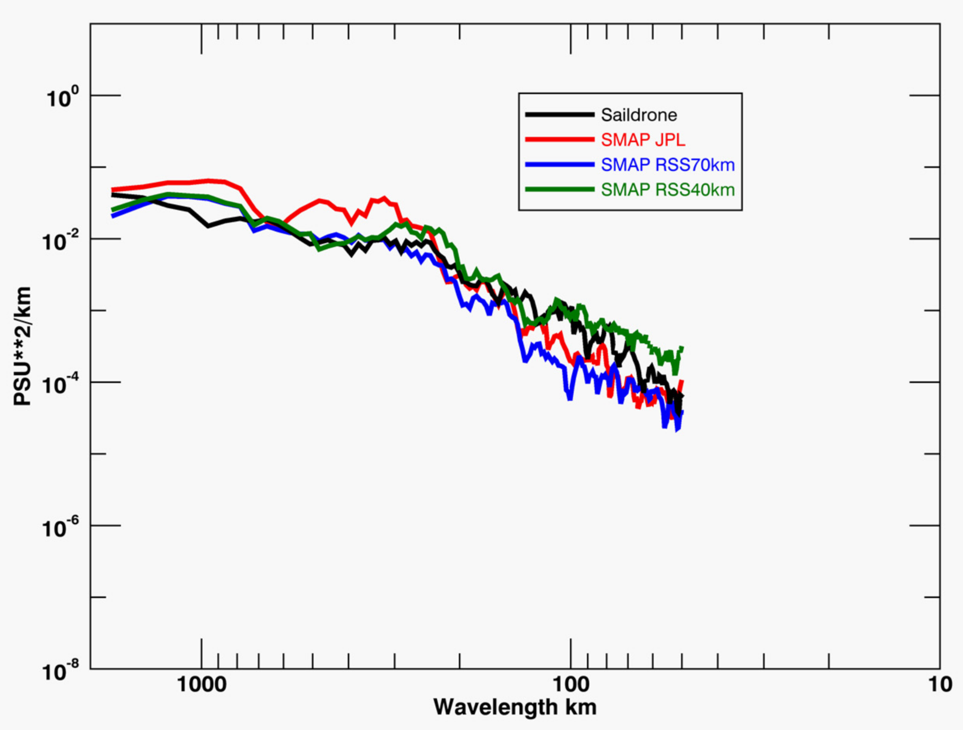
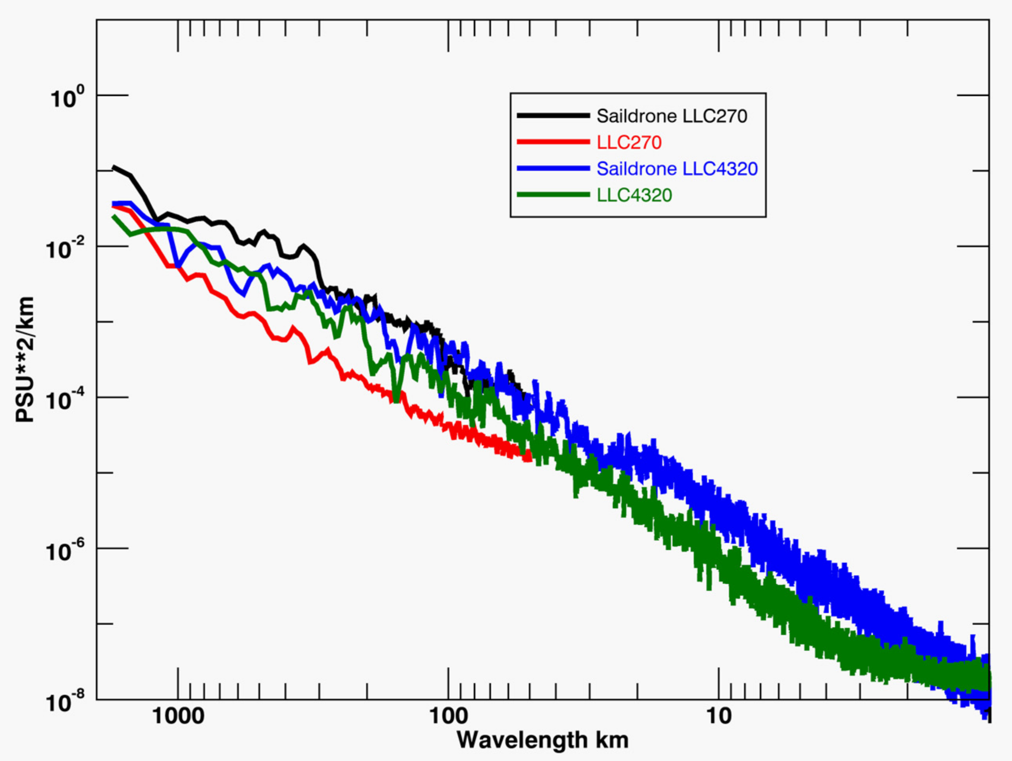
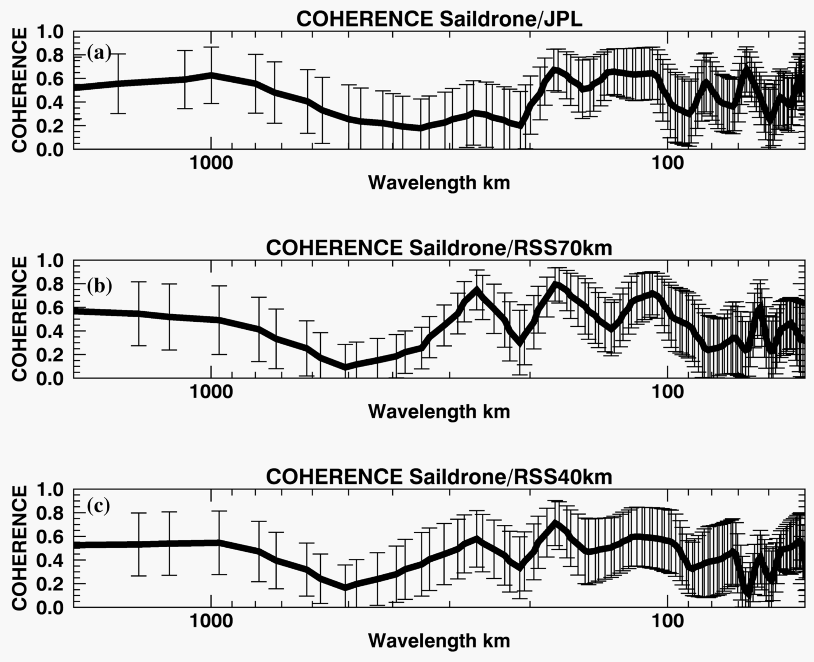
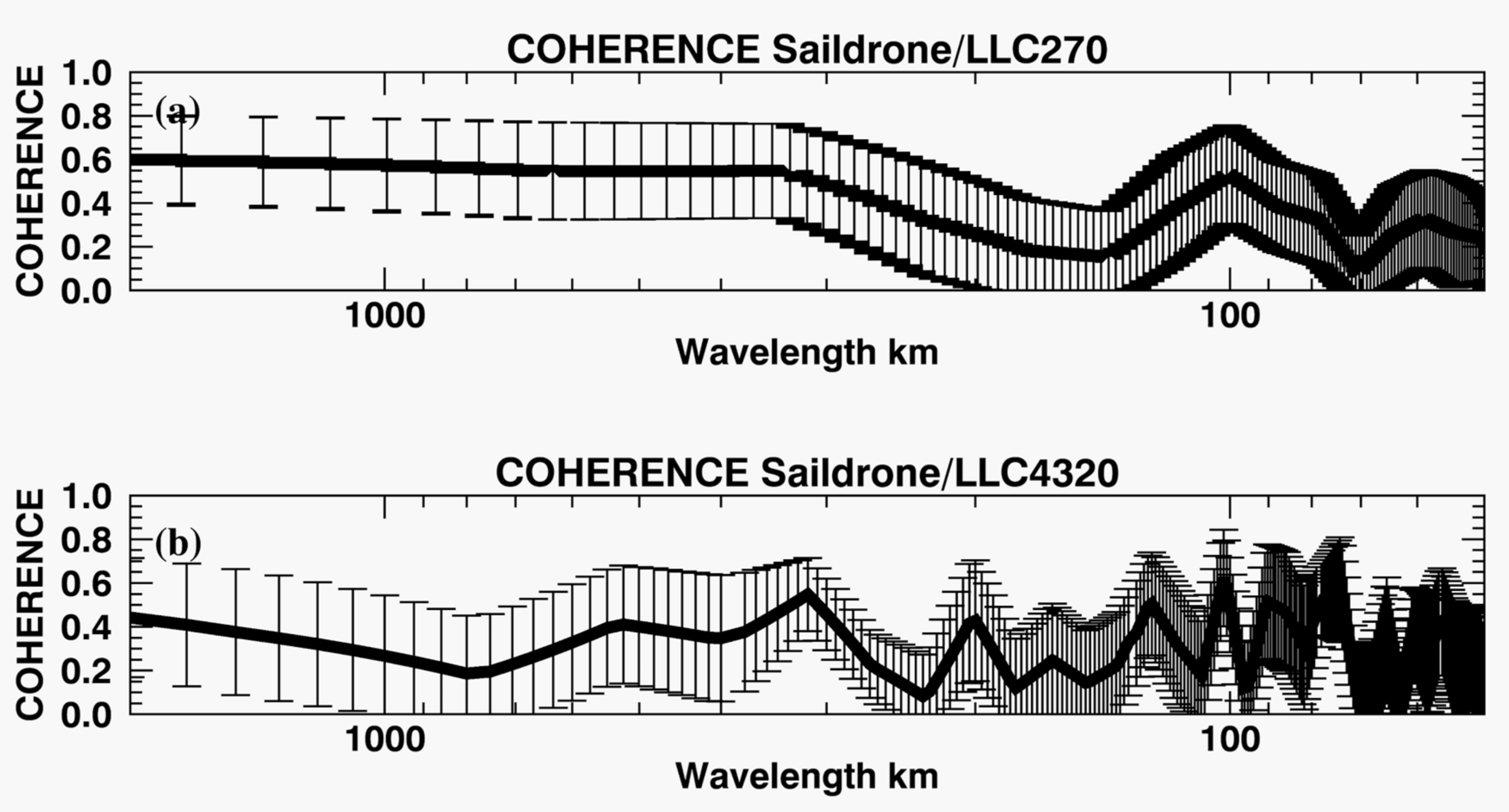
3.3. Spectra and Coherences

To further quantify the results from the time series, spectra and coherence statistics (inclusive of the spectral slopes) were calculated. The intent is not to determine a “best” data set, but to present statistics that can guide the best use of and improvement in SMAP data and models in the Bering, Chukchi, and Beaufort Seas.
Spectra and coherences were derived for the three SMAP SSS products and LLC270/LLC4320 models, and then compared directly with the Saildrone SSS. The spectra and coherences were first calculated individually for the SMAP-, model-, and Saildrone-derived SSS for the two Saildrone deployments, SD1036 and SD1037. Coherences were derived between each of the SMAP/model products and the Saildrone matchups. The spectra and coherences were then averaged for the two deployments. Figure 5 shows the spectra for the three SMAP products (JPLSSS, RSS40km, and RSS70km) compared with the Saildrone-derived SSS. Figure 5 (red) shows higher values for the JPLSSS spectra, compared to Saildrone, at wavelengths >300 km. Figure 5 (blue) shows the RSS70km versus Saildrone. In general, the spectra follow each other except at approximately 100 km. This is most likely due to resolving of the coastal freshening signal, where the RSS70km provides a smoother estimate. Figure 5 (green) shows the spectra for the RSS40km and Saildrone. Overall, the RSS40km spectra follows the Saildrone spectra until approximately 100 km, where the RSS40km spectral densities are larger than the Saildrones. This would be consistent with increased noise in the RSS40km over the smoother JPLSSS and RSS70km products. Figure 6 shows the spectral plots for LLC270 (red) and LLC4320 (green) compared with the Saildrone SSS. All SMAP observations are gridded at 0.25°, while LLC4320 is approximately 1 km, which is reflected in the LLC4320 spectra being extended to 1 km.
The decreased spectral densities associated with LLC270 are clearly indicative that lower-resolution LLC270 does not fully resolve the spatial variability/dynamics of the region. Figure 6 (green) shows the spectral densities for the higher resolution LLC4320 and Saildrones. LLC4320 matches better, but is overall still lower than the Saildrone SSS spectral density. The difference between the two models clearly shows the importance of the higher-resolution LLC4320 model in fully resolving the dynamics of the Alaskan coast, including mesoscale-to-submesoscale variability. Additionally, LLC4320 shows a white spectrum at ~5 km, while the spectra of Saildrone continues with a consistent slope. Thus, Saildrone spectral density is indicative of variability that still exists at <5 km that is not resolved by LLC4320, although the high-resolution model is resolving more of the variability along the Alaskan coast than either the SMAP products or the lower-resolution LLC270. The separation of the spectral densities for the RSS40km and RSS70km products at approximately 100 km would be consistent with a Nyquist wavelength of approximately 100 km for the SMAP SSS products. Based on the smoothing used for the JPLSSS product, the feature resolution is approximately 60 km, leading to a Nyquist frequency of approximately 120 km. This compares to a feature resolution of 40 km for the RSS40km product and 70 km for the RSS70km product, consistent with results in [9]. Further comparisons of spectral slopes will be analyzed in the discussion section.
To further examine the statistical relationships between the SMAP/Model SSS and the Saildrone SSS, coherences were derived. Figure 7a–c shows the coherence between the three products and the Saildrone. The JPLSSS product shows that coherence of approximately 0.60 exists for wavelengths >1000 km, with a drop off at wavelengths <1000 km, increasing again at 200 km and remaining statistically significant up through 50 km. Error bars indicate the statistical significance of the coherence. Highest coherences are seen at 50 and 70 km, with a minimum visible at 60 km. Coherences at <50 km are not shown, as error bars indicate no statistical significance. Figure 7b shows the coherences for the RSS70km product. Overall, the coherences follow similar patterns as the JPLSSS product, but with lower coherences. Coherences peak at roughly 0.8 for RSS70km, 0.7 for JPLSSS, and 0.6 for RSS40km. The decreased coherences could be due to the RSS70km being the smoothest of the three SMAP products; this is consistent with RSS40km containing greater noise. Figure 7c shows the coherence for the RSS40km product. The pattern is similar to the JPLSSS and RSS70km products, with coherences peaking at approximately 0.7. Coherences <50 km became statistically insignificant. Overall, the coherences for the three SMAP SSS products followed similar patterns with maxima coherences seen between 300 and 100 km. Coherences decreased at wavelengths less than 100 km, consistent with the Nyquist wavelength for the SMAP SSS products.
Figure 8a,b shows coherences for LLC270 and LLC4320. The smoothness of the LLC270 coherence is due to the lower resolution of the model. LLC270 shows overall coherences of 0.6 between 1000–200 km. A peak exists at 100 km before the coherences become statistically insignificant. Coherences for LLC4320 also show statistically significant coherences between 300 and 1000 km, peaking at approximately 0.6. The major differences are three significant peaks found between 100 and 50 km. These significant peaks at <100 km are most likely due to the higher resolution of LLC4320. The peaks are consistent with those found in the JPLSSS and RSS70km coherences. The similarity in peaks between the SMAP and model coherences indicates a consistency between the satellite-derived SSS and model SSS in resolving features off the Alaskan coast. As with the SMAP-derived values, coherences of < 50 km were found to be statistically insignificant based on the error bars.

4. Discussion

To further identify and quantify the differences between the datasets, biases, correlations, and RMSD were derived between the SMAP-, model-, and Saildrone-derived SSS. Slopes of the spectra were also derived for each of the data sets. Table 1 summarizes the SSS correlations, biases, and RMSD for SMAP, LLC270, and LLC4320 versus Saildrones.
Overall, the RSS70km product performs the best with correlations of 0.95 and 0.92 for SD1037 and SD1038, respectively. Additionally, biases near 0.02 and RMSD of 0.72 and 0.89 indicate good agreement between the RSS70km and Saildrone. RSS40km has correlations of 0.93 and 0.90 with smaller biases of 0.03 and 0.005. From the correlation analysis, bias, and RMSD, the RSS40km and RSS70km products performed similarly. Based on the spectra, the RSS40km product has increased noise at higher wavelengths. This would be consistent with values closer to the coast and increased land contamination. This result is encouraging, as it indicates that the higher resolution of the RSS40km does not significantly degrade the signal off the Alaskan coast. This demonstrates that RSS40km does not add significant noise when compared to the RSS70km product. This could be a result of the signal being dominated by the large Yukon River discharge plume and coastal dynamics of the region. Thus, the smoother RSS70km approach does not significantly impact the correlations. Overall, the JPLSSS product has lower correlations of 0.82 and 0.84 with biases of approximately 0.6 and 0.4 PSU for SD1036 and SD1037, respectively (RMSD values were 1.99 and 1.77) Most likely the lower correlations and larger biases and RMSD are due to the large freshening seen in the JPLSSS at day 170. However, this could be due to a real signal and should not be considered an indicator that the JPLSSS is underperforming compared to the other products.
Correlations for LLC270 were 0.83 and 0.79 for SD1036 and SD1037, respectively. Biases were 0.49 and 0.66 PSU, with RMSD 1.10 and 1.22 PSU. The higher-resolution LLC4320 shows correlations of 0.82 and 0.97, with biases of 0.38 and 0.03 PSU. RMSD differences were 1.37 and 1.45. These results indicate that the higher-resolution model, especially with the 0.97 correlation, resolves additional fine-scale variability not seen with the lower-resolution LLC270. Additionally, the biases and RMSD of the SMAP products are consistent with what was found by [5] for comparisons with in-situ data above 65°N. RSS70km had correlations greater than 0.9, with JPLSSS being 0.84.
To compare the spectra, slopes were derived for each of the SMAP/model/Saildrone spectra. The slopes were derived over a wavelength of 100–1000 km. Table 2 summarizes the derived slopes for each of the spectra. Previous studies [8] comparing SMAP SSS with Saildrone off the California/Baja Coast have shown spectral slopes that approximate the −2 slopes associated with mesoscale-to-submesoscale variability [8,37,38].
The spectral slopes of the RSS40km product compared best with those of Saildrone. The spectral slope for the RSS40km was −1.93, while for Saildrone was −2.26. The JPLSSS product had the steepest slope of −2.95. The steeper slopes are most likely indicative of the smoother product and decreased energy associated with scales <100 km. Thus, this would be consistent with the known feature resolutions of the products, with RSS40km having a 40 km and RSS70km and JPLSSS having 70 km and 60 km feature resolutions, respectively. The Saildrone SSS spectral slope of −2.26 reflects the slope most closely associated with mesoscale-submesoscale variability [8].
When compared with Saildrone, the model spectral slopes also approximated the −2 slopes associated with mesoscale-submesoscale variability. LLC270 had a spectral slope −1.81, while the co-located Saildrone SSS had a spectral slope of −2.13. The lower spectral slope of LLC270 is most likely a function of the smoother LLC270 SSS due to the lower resolution of the model. LLC4320 has a spectral slope of −2.32, while the Saildrone co-located SSS had a spectral slope of −2.04. Thus, the Saildrone SSS spectra slope co-located with the high resolution LLC4320 model was the closest to the known slopes of −2.0 associated with the mesoscale-to-submesoscale dynamics. The steeper −2.32 slope is consistent with the model slightly underestimating higher-resolution variability.
Overall, the values of the satellite and model spectral slopes are consistent with the Saildrone slopes, with the differences being consistent with the smoothing levels and feature resolutions of the products. The comparisons between LLC270 and LLC4320 models clearly indicate that the higher-resolution LLC4320 model resolves features not obtained with the lower-resolution SMAP and LLC270 resolutions at wavelengths <10 km.
The fine spatiotemporal resolution of Saildrone provides the ability to directly assess and validate the monitoring capabilities of satellite-derived SST, SSS, and biogeochemical properties in the critical Arctic regions. The spectra and coherence of the LLC4320 model compared to Saildrone indicates that significant variability exists at scales <100 km, providing justification for future studies. Additionally, work is already being conducted comparing biogeochemical Saildrone observations with the ECCO-Darwin global-ocean biogeochemistry model [39]. The integration of Saildrone and satellite observations is critical for advancing research in both physical and biological oceanography. These results also indicate the need to continually improve land correction, with a focus on increasing retrievals closer to land. This would lead to a more accurate characterization of river runoff based on land ice and snow melt.

5. Conclusions and Summary

Two 2019 Saildrone deployments in the Bering, Chukchi, and Beaufort Seas off the Alaskan coast allowed for direct comparisons between the SSS derived from the onboard RBR and SSS derived from three SMAP products and two state-of-the-art numerical ocean models.
The most dominant feature of the time series was a strong freshening event at approximately day 150 of 2019. This event was visible in all the SMAP products and the Saildrone SSS. Saildrone was first used to detect discharge associated with the Yukon with deployments in 2015 [40]. Based on collocation with the Yukon River discharge, it was determined that the freshening event was associated with river runoff. Figure 1 and Figure 2 clearly show the freshening event along the coast. Figure 2 zooms in on the region of the river discharge, showing the freshening in the Saildrone SSS as it crosses the region. All the SMAP SSS products resolve the signal associated with the Yukon River. This result is essential in motivating future Arctic Ocean research using Saildrone and satellite-derived SSS for the determination of freshwater fluxes and changes in ocean stratification due to both sea-ice melt and river runoff. Previous results have used remote sensing [9] to determine and monitor the discharge of the Yukon River. To our knowledge, this is the first time satellite-derived SSS has been used to detect the freshening in the Bering Sea associated with the Yukon River. The results are consistent, appearing on day 150 of 2019, with the known seasonal discharge of the Yukon River peaking in boreal summer [39] with 5663 m3 s−1. Thus, these results are encouraging for application of satellite-derived salinity to monitor changes in the Yukon River discharge plume associated with changes in sea-ice melt, shelf dynamics, and freshwater discharge. This could prove critical for understanding future changes in the Arctic and applications to other regions.
Overall, the comparisons showed good agreement between the JPLSSS, RSS40km, and RSS70km products. Correlations of greater than 0.9 were found for the RSS70km and RSS40km products. Biases of near 0 PSU were found for the RSS40km and RSS70km products, with RMSD of < 1.0 PSU. Values were comparable to those found by [5,6], who compared satellite-derived SSS products in the Arctic using thermosalinograph (TSG) data. Overall spectral slopes compared well and approximated the −2.0-slope associated with mesoscale-to-submesoscale processes. Slopes for the JPLSSS and RSS70km were steeper than Saildrone SSS, most likely indicative of the smoothness of the two SMAP products. Model spectral slopes compared with Saildrone SSS were also consistent with the feature resolutions of the LLC270 and LLC4320 models.
Both SMAP/Model showed statistically significant coherences with Saildrone SSS. Peaks were seen at 100–500 km, as well as 50 km for the SMAP observations; LLC270 showed reduced coherences. The commonality of peaks at approximately 100 km could be associated with the Yukon River discharge, but confirmation of this is beyond the scope of this paper and should be a topic for future research.
Validation results should be considered a first step in using SMAP and Saildrone in the Arctic Ocean. Statistically significant correlations and negligible biases are promising for future high-latitude applications. Biases were larger for the JPLSSS product, most likely due to a large freshening event between days 160 and 170. Future work in the Arctic should include comparisons with additional Saildrone campaigns as well as with data from the European Space Agency’s Soil Moisture Ocean Salinity mission. The coherences associated with the high-resolution LLC4320 model indicate that both improvements in resolution and land contamination are critical for fully resolving ocean variability in the Bering, Chukchi, and Beaufort Seas. The clear resolution of the Yukon River discharge is promising to use SMAP to monitor changes in fresh shelf water influence on the large-scale salinity of the Bering, Chukchi, and Beaufort Seas. Future research should focus on (1) improving derivations of satellite-derived SSS in the Arctic Ocean and (2) integrating models to compliment the remote sensing with the full response of the Arctic region to climate change. Ultimately, Saildrone provides a unique opportunity for validating and improving remote sensing products in the Arctic and other high-latitude regions. Future work needs to explore further differences in the SMAP products, inclusive of the large freshening even observed in the JPLSSS at day 170. This should include future exploration of differences in SSS close to land and possible issues with the SMAP instrument malfunction. Additional work should include the incorporation of comparisons with the European Space Agency’s Soil Moisture Ocean Salinity Mission (SMOS).

Supplementary Materials

The following are available online at https://www.mdpi.com/2072-4292/13/5/831/s1, Figure S1. The Figure shows comparisons between the Seabird and RBR salinity measurements.

Author Contributions

Project Administration, J.V.-C.; Preparation, Conceptualization, Investigation, J.V.-C., C.G., W.T.; M.S., D.C. and H.Z.; Conceptualization, D.M., J.G.-V. and M.B.; Editing, J.G.-V., M.B. and M.S. All authors have read and agreed to the published version of the manuscript.

Funding

This research was supported by the NASA Salinity Continuity Program. J. Vazquez-Cuervo and Wenqing Tang were funded under contract with NASA at the Jet Propulsion Laboratory/California Institute of Technology. JGV was supported by CICESE and CONACYT, México. MB was supported through the University of Sao Paolo. MS and CG were funded by the MISST3 Project, NASA grant 80NSSC20K0768. MS was also partially supported by NASA Grant to JPL via subcontract 1587724. We also thank three anonymous reviewers for their thorough and thoughtful reviews of this manuscript, which significantly improved the manuscript. We also thank Vardis Tsontos at the Jet Propulsion Laboratory for his editorial support and sharing expertise of the SMAP products.

Data Availability Statement

Not applicable.

Acknowledgments

The three SMAP products, along with the two Saildrone deployments, were downloaded from NASA’s Physical Oceanography Distributed Active Archive Center (PO. DAAC). The JPLSSS product was downloaded from: https://podaac.jpl.nasa.gov/dataset/SMAP_JPL_L3_SSS_CAP_MONTHLY_V43?ids=&values=.The Remote Sensing System products may be downloaded from:https://podaac.jpl.nasa.gov/dataset/SMAP_JPL_L3_SSS_CAP_8DAY-RUNNINGMEAN_V43?ids=&values=. Saildrone data used in this study can also be downloaded through the PO. DAAC at: https://podaac.jpl.nasa.gov/dataset/SAILDRONE_ARCTIC?ids=&values=.

Conflicts of Interest

The authors declare no conflict of interest.

References

  1. Rogers, L.A.; Wilson, M.T.; Duffy-Anderson, J.T.; Kimmel, D.G.; Lamb, J.F. Pollock and “the Blob”: Impacts of a marine heatwave on walleye pollock early life stages. Fish. Oceanogr. 2020. Early View. [Google Scholar] [CrossRef]
  2. Sambrotto, R.N.; Mordy, C.; Zeeman, S.I.; Stabeno, P.J.; Macklin, S.A. Physical forcing and nutrient conditions associated with patterns of Chl and phytoplankton productivity in the southeastern Bering Sea during summer. Deep-Sea Res. Part Ii-Top. Stud. Oceanogr. 2008, 55, 1745–1760. [Google Scholar] [CrossRef]
  3. Walsh, J.J.; McRoy, C.P. Ecosystem Analysis in the Southeastern Bring Sea. Cont. Shelf Res. 1986, 5, 259–288. [Google Scholar] [CrossRef]
  4. Strom, S.L.; Fredrickson, K.A. Intense stratification leads to phytoplankton nutrient limitation and reduced microzooplankton grazing in the southeastern Bering Sea. Deep-Sea Res. Part Ii-Top. Stud. Oceanogr. 2008, 55, 1761–1774. [Google Scholar] [CrossRef]
  5. Fournier, S.; Lee, T.; Tang, W.Q.; Steele, M.; Olmedo, E. Evaluation and Intercomparison of SMOS, Aquarius, and SMAP Sea Surface Salinity Products in the Arctic Ocean. Remote Sens. 2019, 11, 3043. [Google Scholar] [CrossRef] [Green Version]
  6. Tang, W.Q.; Yueh, S.; Yang, D.Q.; Fore, A.; Hayashi, A.; Lee, T.; Fournier, S.; Holt, B. The potential and challenges of using Soil Moisture Active Passive (SMAP) sea surface salinity to monitor Arctic Ocean freshwater changes. Remote Sens. 2018, 10, 869. [Google Scholar] [CrossRef] [Green Version]
  7. Bjerklie, D.M.; Birkett, C.M.; Jones, J.W.; Carabajal, C.; Rover, J.A.; Fulton, J.W.; Garambois, P.A. Satellite remote sensing estimation of river discharge: Application to the Yukon River Alaska. J. Hydrol. 2018, 561, 1000–1018. [Google Scholar] [CrossRef] [Green Version]
  8. Vazquez-Cuervo, J.; Gomez-Valdes, J.; Bouali, M.; Miranda, L.E.; Van der Stocken, T.; Tang, W.Q.; Gentemann, C. Using Saildrones to Validate Satellite-Derived Sea Surface Salinity and Sea Surface Temperature along the California/Baja Coast. Remote Sens. 2019, 11, 1964. [Google Scholar] [CrossRef] [Green Version]
  9. Fore, A.G.; Yueh, S.H.; Tang, W.Q.; Stiles, B.W.; Hayashi, A.K. Combined Active/Passive Retrievals of Ocean Vector Wind and Sea Surface Salinity With SMAP. IEEE Trans. Geosci. Remote Sens. 2016, 54, 7396–7404. [Google Scholar] [CrossRef]
  10. Meissner, T.; Wentz, F.J.; Le Vine, D.M. The Salinity Retrieval Algorithms for the NASA Aquarius Version 5 and SMAP Version 3 Releases. Remote Sens. 2018, 10, 1121. [Google Scholar] [CrossRef] [Green Version]
  11. Gentemann, C.L.; Scott, J.P.; Mazzini, P.L.F.; Pianca, C.; Akella, S.; Minnett, P.J.; Cornillon, P.; Fox-Kemper, B.; Cetinic, I.; Chin, T.M.; et al. Saildrone: Adaptively sampling the marine environment. Bull. Am. Meteorol. Soc. 2020, 2020, 744–762. [Google Scholar] [CrossRef] [Green Version]
  12. Zhang, H.; Menemenlis, D.; Fenty, I.G. ECCO LLC270 Ocean-Ice State Estimate. Available online: http://hdl.handle.net/1721.1/119821 (accessed on 1 June 2020).
  13. Forget, G.; Campin, J.M.; Heimbach, P.; Hill, C.N.; Ponte, R.M.; Wunsch, C. ECCO version 4: An integrated framework for non-linear inverse modeling and global ocean state estimation. Geosci. Model Dev. 2015, 8, 3071–3104. [Google Scholar] [CrossRef] [Green Version]
  14. Menemenlis, D.; Campin, J.; Heimbach, P.; Hill, C.; Lee, T.; Nguyen, A.; Schodlock, M.; Zhang, H. ECCO2: High resolution global ocean and sea ice data synthesis. Mercator Ocean Q. Newsl. 2008, 31, 13–21. [Google Scholar]
  15. Fenty, I.; Menemenlis, D.; Zhang, H. Global coupled sea ice-ocean state estimation. Clim. Dyn. 2017, 49, 931–956. [Google Scholar] [CrossRef]
  16. Fekete, B.M.; Vorosmarty, C.J.; Grabs, W. High-resolution fields of global runoff combining observed river discharge and simulated water balances. Glob. Biogeochem. Cycles 2002, 16. [Google Scholar] [CrossRef]
  17. Redi, M.H. Oceanic Isopycnal Mixing by Coordinate Rotation. J. Phys. Oceanogr. 1982, 12, 1154–1158. [Google Scholar] [CrossRef] [Green Version]
  18. Gent, P.R.; McWilliams, J.C. Isopycnal mixing in ocean circulation models. J. Phys. Oceanogr. 1990, 20, 150–155. [Google Scholar] [CrossRef] [Green Version]
  19. Forget, G.; Ponte, R.M. The partition of regional sea level variability. Prog. Oceanogr. 2015, 137, 173–195. [Google Scholar] [CrossRef] [Green Version]
  20. Andersen, O.; Knudsen, P.; Stenseng, L. The DTU13 MSS (Mean Sea Surface) and MDT (Mean Dynamic Topography) from 20 years of satellite altimetry. In IGFS 2014 International Association of Geodesy Symposia; Jin, S., Barzaghi, R., Eds.; Springer: Cham, Switzerland, 2015; Volume 144, pp. 111–121. [Google Scholar]
  21. Watkins, M.M.; Wiese, D.N.; Yuan, D.N.; Boening, C.; Landerer, F.W. Improved methods for observing Earth’s time variable mass distribution with GRACE using spherical cap mascons. J. Geophys. Res. Solid Earth 2015, 120, 2648–2671. [Google Scholar] [CrossRef]
  22. Reynolds, R.W.; Rayner, N.A.; Smith, T.M.; Stokes, D.C.; Wang, W.Q. An improved in situ and satellite SST analysis for climate. J. Clim. 2002, 15, 1609–1625. [Google Scholar] [CrossRef]
  23. Meier, W.; Fetterer, F.; Savoie, M.; Mallory, S.; Duerr, R.; Stroeve, J. NOAA/NSIDC Climate Data Record of Passive Microwave Sea Ice Concentration, Version 3. Available online: https://nsidc.org/data/G02202/versions/3 (accessed on 1 June 2020).
  24. Roemmich, D.; Gilson, J. The 2004–2008 mean and annual cycle of temperature, salinity, and steric height in the global ocean from the Argo Program. Prog. Oceanogr. 2009, 82, 81–100. [Google Scholar] [CrossRef]
  25. Riser, S.C.; Swift, D.; Drucker, R. Profiling Floats in SOCCOM: Technical Capabilities for Studying the Southern Ocean. J. Geophys. Res. Ocean 2018, 123, 4055–4073. [Google Scholar] [CrossRef]
  26. Locarnini, R.; Mishonov, A.; Boyer, T.; Garcia, H.; Baranova, O. World Ocean Atlas 2009, Volume 1: Temperature. In NOAA Atlas NESDIS; U.S. Government Printing Office: Washington, DC, USA, 2010; Volume 68. [Google Scholar]
  27. Antonov, J.; Seidov, D.; Boyer, T.; Locarnini, R.; Mishonov, A.; Garcia, H. World Ocean Atlas 2009, Volume 2: Salinity. In NOAA Atlas NESDIS; U.S. Government Printing Office: Washington, DC, USA, 2010; Volume 69. [Google Scholar]
  28. Roquet, F.; Wunsch, C.; Forget, G.; Heimbach, P.; Guinet, C.; Reverdin, G.; Charrassin, J.B.; Bailleul, F.; Costa, D.P.; Huckstadt, L.A.; et al. Estimates of the Southern Ocean general circulation improved by animal-borne instruments. Geophys. Res. Lett. 2013, 40, 6176–6180. [Google Scholar] [CrossRef] [Green Version]
  29. Treasure, A.M.; Roquet, F.; Ansorge, I.J.; Bester, M.N.; Boehme, L.; Bornemann, H.; Charrassin, J.B.; Chevallier, D.; Costa, D.P.; Fedak, M.A.; et al. Marine Mammals Exploring the Oceans Pole to Pole A Review of the MEOP Consortium. Oceanography 2017, 30, 132–138. [Google Scholar] [CrossRef]
  30. Krishfield, R.; Toole, J.; Proshutinsky, A.; Timmermans, M.L. Automated Ice-Tethered Profilers for Seawater Observations under Pack Ice in All Seasons. J. Atmos. Ocean. Technol. 2008, 25, 2091–2105. [Google Scholar] [CrossRef]
  31. Wunsch, C.; Heimbach, P. Dynamically and kinematicaly consistent global ocean circulation and ice state estimates. In Ocean Circulation and Climate: A 21st Century Perspective; Siedler, G., Church, J., Gould, J., Griffies, S., Eds.; Elsevier: Amsterdam, The Netherlands, 2013; pp. 553–579. [Google Scholar]
  32. Wunsch, C.; Heimbach, P.; Ponte, R.M.; Fukumori, I.; Members, E.-G.C. The global general circulation of the ocean estimated by the ecco-consortium. Oceanography 2009, 22, 88–103. [Google Scholar] [CrossRef]
  33. Dee, D.P.; Uppala, S.M.; Simmons, A.J.; Berrisford, P.; Poli, P.; Kobayashi, S.; Andrae, U.; Balmaseda, M.A.; Balsamo, G.; Bauer, P.; et al. The ERA-Interim reanalysis: Configuration and performance of the data assimilation system. Q. J. R. Meteorol. Soc. 2011, 137, 553–597. [Google Scholar] [CrossRef]
  34. Hoyer, S.; Hamman, J.; Roos, M.; Cherian, D.; Fitzgerald, C.; Fujii, K.; Maussion, F.; Crusaderky, K.; Kleeman, A.; Clark, S.; et al. Pydata/xarray: v0.16.0. Available online: https://zenodo.org/record/3940662#.YDW54It62Uk (accessed on 1 June 2020).
  35. Tang, W.; Simon, H.; Yueh, S.H.; Alexander, G.; Akiko, K. An Empirical Sea Ice Correction Algorithm for SMAP SSS Retrieval in the Arctic Ocean. In Proceedings of the IGARSS 2020-2020 IEEE International Geoscience and Remote Sensing Symposium, Waikoloa, HI, USA, 26 September–2 October 2020; pp. 5639–5642. [Google Scholar]
  36. Vazquez-Cuervo, J.; Gomez-Valdes, J.; Bouali, M. Comparison of satellite-driven sea surface temperature and sea surface salinity gradients using the Saildrone California/Baja and North Atlantic Gulf Stream deployments. Remote Sens. 2020, 12, 1839. [Google Scholar] [CrossRef]
  37. Castro, S.L.; Monzon, L.A.; Wick, G.A.; Lewis, R.D.; Beylkin, G. Subpixel variability and quality assessment of satellite sea surface temperature data using a novel High Resolution Multistage Spectral Interpolation (HRMSI) technique. Remote Sens. Environ. 2018, 217, 292–308. [Google Scholar] [CrossRef]
  38. Castro, S.L.; Wick, G.A.; Steele, M. Validation of satellite sea surface temperature analyses in the Beaufort Sea using UpTemp buoys. Remote Sens. Environ. 2016, 187, 458–475. [Google Scholar] [CrossRef]
  39. Carroll, D.; Menmenlis, D.; Adkins, J.F.; Bowman, K.W.; Brix, H.; Dutkiewicz, S.; Fenty, I.; Gierach, M.M.; Hill, C.; Jahn, O.; et al. The ECCO-Darwin Data-Assimilative Global Ocean. Biogeochemistry Model: Estimates of Seasonal to Multidecadal Surface Ocean. pCO2 and Air-Sea CO2 Flux. J. Adv. Model. Earth Syst. 2020, 12, e2019MS001888. [Google Scholar] [CrossRef]
  40. Brabets, T.P.; Wang, B.; Meade, R.H. Environmental and Hydrologic Overview of the Yukon River Basin, Alaska and Canada; United States Geological Survey: Reston, VA, USA, 2000. [Google Scholar]
Figure 1. Maps of mean SSS time-averaged over the period of Saildrone deployment. (a) SMAP JPL V4.3, (b) SMAP RSS 70km, (c) SMAP RSS 40km, (d) LLC270, and (e) LLC4320. Blue values are indicative of low salinity. Overlaid are tracks of Saildrone 1036 (black) and 1037 (grey) deployments. White colors indicate satellite data that was masked due to land contamination. The locations of Saildrones when the two major freshening events occurred (see Figure 2) are indicated by red diamond symbols. (f) shows a map with the geographical locations of the study area, including the location of the Yukon River discharge (Y-K delta).
Remotesensing 13 00831 g001
Figure 2. (a) Map of mean SSS derived from RSS70km product over the period of the Saildrone deployment. (b) Saildrone SSS from SD1036 along the deployment track. Blue arrow shows the location of Y-K Delta.
Remotesensing 13 00831 g002
Figure 3. Time series of salinity measured by RBR sensor on (a) Saildrone 1036 and (b) Saildrone 1037 (in original Saildrone sampling rate) and collocated SMAP SSS and model outputs. Dotted vertical lines indicate the period of two major freshening events (see text).
Remotesensing 13 00831 g003
Figure 4. Scatterplot of salinity measured by the RBR sensor on (a) Saildrone 1036 and (b) Saildrone 1037 (average of all Saildrone measurements corresponding to the same satellite/model collocation) and collocated SMAP SSS and model outputs. Same color code is used for each product as in the time series of Figure 2.
Remotesensing 13 00831 g004
Figure 5. Wavenumber spectra for SMAP products and Saildrone.
Remotesensing 13 00831 g005
Figure 6. Wavenumber spectra for LLC270 and LLC4320. Differences between the SMAP/Saildrone spectra and the model/Saildrone comparisons can be explained by the different model resolutions.
Remotesensing 13 00831 g006
Figure 7. (a) Coherence for JPLSSS/Saildrone, (b) coherence for RSS40km/Saildrone, and (c) coherence for RSS70km/Saildrone.
Remotesensing 13 00831 g007
Figure 8. (a) Coherence for LLC270/Saildrone and (b) coherence for LLC4320/Saildrone.
Remotesensing 13 00831 g008
Table 1. Statistics for Saildrone/SMAP/model comparisons. Rows correspond to the specific SMAP product and model versus Saildrone comparison for each specific deployment.
ParameterCorrelationBias (PSU)RMSD (PSU)
JPLSSS
1036
0.820.661.34
JPLSSS
1037
0.840.421.24
RSS70km
1036
0.950.040.73
RSS70km
1037
0.92−0.030.89
RSS40km
1036
0.930.030.88
RSS40km
1037
0.91−0.0050.98
LLC270
1036
0.830.491.11
LLC270
1037
0.790.671.22
LLC4320
1036
0.820.391.37
LLC4320
1037
0.970.031.45
Table 2. Corresponding spectral slopes. Parameter/Sail indicates the slope of the Saildrone SSS collocated with that parameter.
ParameterSlope
JPL/Sail−2.26
JPL−2.96
RSS70km/Sail−2.26
RSS70km−2.67
RSS40km/Sail−2.26
RSS40km−1.93
LLC270/Sail−2.14
LLC270−1.81
LLC4320/Sail−2.05
LLC4320−2.32
Publisher’s Note: MDPI stays neutral with regard to jurisdictional claims in published maps and institutional affiliations.

