Abstract
The article presents a methodology for examining a temporal sequence of synthetic aperture radar (SAR) images, as applied to the detection of the A-68 iceberg and its drifting trajectory. Using an improved image processing scheme, the analysis covers a period of eighteen months and makes use of a set of Sentinel-1 images. A-68 iceberg calved from the Larsen C ice shelf in July 2017 and is one of the largest icebergs observed by remote sensing on record. After the calving, there was only a modest decrease in the area (about 1%) in the first six months. It has been drifting along the east coast of the Antarctic Peninsula, and is expected to continue its path for more than a decade. It is important to track the huge A-68 iceberg to retrieve information on the physics of iceberg dynamics and for maritime security reasons. Two relevant problems are addressed by the image processing scheme presented here: (a) How to achieve quasi-automatic analysis using a fuzzy logic approach to image contrast enhancement, and (b) The use of ferromagnetic concepts to define a stochastic segmentation. The Ising equation is used to model the energy function of the process, and the segmentation is the result of a stochastic minimization.
1. Introduction
Weather conditions and seasonal variations impose restrictions on the monitoring of Antarctica by satellite remote sensing. Continuous sunlight from December to February makes it a good period for optical image remote sensing. However, clouds, snow and ice elements all display a similar spectral signature in both optical and thermal wavelengths. Antarctica has seven months of winter darkness, from March to September. During the Antarctic night, both synthetic aperture radar (SAR) and infra-red images can monitor ice coverage, however, cloudy weather makes infra-red observation impossible. The scatterometer is an alternative instrument, but because of its low spatial resolution, it can only give rough estimations of large icebergs. Consequently, continuous monitoring of Antarctica can only be carried out by SAR imaging systems. This paper gives an example of Antarctic monitoring by analysing some elements of the drifting trajectory of the A-68A iceberg using Sentinel-1 SAR data.
The fracture of the Antarctic Larsen C ice shelf occurred in 2017 between July 10th and 12th, with a loss of some 5800 km corresponding to about 12% of the entire shelf area. The giant calved iceberg was named “A-68” by the US National Ice Center (USNIC). Later, it broke apart and the largest chunk was named A-68A. It is the sixth largest recorded iceberg, and at present, it is the largest iceberg in the world. Because of its size, an iceberg like A-68A can have a life of several years. Iceberg drifting patterns constitute a risk for navigation and shipping routes. Satellite remote sensing imagery can provide the tool for mapping iceberg trajectory progression.
In iceberg monitoring by remote sensing, there are two basic objectives: iceberg detection and iceberg drifting forecast. For iceberg detection, a hierarchical object-based segmentation is applied to a set of geometrical parameters of ENVISAT/ASAR images [1]. The radar altimeter is an alternative instrument, and in [2], the signatures of icebergs in waveform space are analyzed by threshold criteria to parametrize iceberg distribution. In [3], a machine learning technique is applied to mask clouds in multispectral Landsat images. Then, iceberg detection is performed by threshold criteria, being careful to notice the radiometric contrast between icebergs and the surrounding open sea. Using Sentinel-1 SAR and CryoSat-2 SIRAL data, Han et al. [4] describe the topological evolution of iceberg A68 and investigate the effects of environmental forces over a period of 18 months. A review of the remote sensing of the cryosphere and processing techniques for sea ice can be found in [5,6].
For iceberg and ice tracking forecasting, an unmanned aerial vehicle platform was used to analyse thermal video [7]. A set of dynamic forecasts was obtained, using GPS trackers positioned on icebergs in [8]. Based on Sentinel-1 images in [9], non-linear diffusion filtering reduces the speckle noise, and features are detected in a non-linear multiscale space representation; nearest-neighbour matching reveals the connections between the extracted features, these being the basis for sea ice drift tracking. In another study [10], the Sentinel-1 SAR image resolution is reduced by a spatial average operation to decrease speckle influence. Then, sea ice tracking is performed using a scale-invariant feature transform algorithm. In a set of ENVISAT/ASAR images, after morphological characterization by pixel-based segmentation, tracking is performed using ocean current data [11]. In [12], a drift model makes use of wind predictions for estimating positions and trajectories of icebergs observed in ENVISAT/ASAR images. More complete delineations, such as the statistical, kinematic and dynamic models, require hydro-meteorological data and both atmosphere and ocean circulation models [13]. In general, modeling the interacting forces is a very complex task [14,15].
With regard to the image processing domain, SAR reconnaissance capabilities are limited by the peculiar behaviour of radar imaging; indeed, basic problems, such as the irregular image contrast and the multiplicative degradation by speckle noise, are still a challenge. Pixel-based techniques, such as k-means, Fuzzy c-means, minimum distance criteria and normalized multi-band indexes are well suited for optical and multi-band images, but their algorithmic performance is limited by the random nature of the SAR data [16]. For this reason, in this paper, the stochastic process theory is taken into account.
For modelling the spatial interaction of pixel data, a model based on concepts of statistical ferromagnetism appears promising. Two relevant problems are addressed by our image processing technique: (a) Low-level fuzzy logic image contrast enhancement, which was derived from medical image analysis, and (b) A segmentation algorithm which considers the random behaviour of the SAR imagery for merging contextual data. A processing scheme was then implemented, which consists of the following steps: (1) Contrast enhancement; (2) Stochastic segmentation, and (3) Measurement of the drift trajectory. Concerning the period of analysis of the iceberg drift, this work was started at the time of the last image of the sequence under analysis. The aim of this study was not to follow the position of the iceberg indefinitely. Our goal was indeed to develop a more effective method to detect iceberg shape and follow its drifting path.
2. Material
This study is based on a set of twelve Sentinel-1 Extra Wide Swath Ground Range Detected (S1 EW GRD, 400 km swath, 20 × 40 m spatial resolution) images at Level-1 in HH polarization; the images were acquired from 22 July 2017 to 26 January 2019, and their geographical coordinates range from latitude 66S to 69S and from longitude 57W to 63W. After retrieval from the ESA Scientific Data Hub, the images were remapped onto a regular grid in stereo-polar projection with a pixel size of 200 × 200 m. The scene size is 400 × 400 km. Figure 1 shows the image corresponding to 22 July 2017, just a few days after the calving event. In Antarctica, most icebergs are created by the calving of ice shelves and glacier tongues. The flat plateau top appearance is a characteristic feature of the tabular icebergs produced in this region.
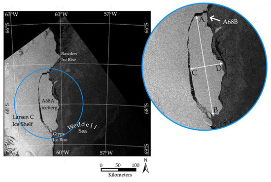
Figure 1.
Sentinel-1 scene of A-68 tabular iceberg acquired on 22 July 2017, only a few days after the calving event. The first derived parameters of this huge tabular iceberg were: the length of its major (segment AB) and minor (segment CD) axes, which were 157.5 km and 47.3 km, respectively.
3. Methods
Electromagnetic variables of radar may introduce undesirable effects in the radiometric quantization so that the grey-level distribution displays a histogram with saturation in local ranges. The subsequent effect is poor image contrast which reduces perception capabilities. Some images in the analyzed data set display this characteristic, and, for this reason, intensity transformation was included in the analysis.
3.1. SAR Scattering
Remote sensing by SAR systems is the result of a complex electromagnetic phenomenon and the radargrammetry technique must consider adverse variables, which may affect the function of the imaging system [17]. The physical manifestation of radar reflectivity is the scattering phenomenon. Diffuse and specular reflections are due to the geometric irregularities of the surface. Other electromagnetic properties, such as the dielectric constant, permeability and conductivity complement the scattering models. These properties modify the rate of the incident and reflected energy. Therefore, the backscattered signal determines the radiometric signature of the scene elements.
At high latitudes, the properties of the scene elements change with time. Geophysical and climatological variables, such as the temperature of the medium, wind speed, rain, salinity and humidity introduce dynamic fluctuations in the scattering phenomenon [18]. For example, new ice produces specular reflections like a thin film with a smooth appearance. Dry snow produces a very weak reflection. Ice sheets and dry soil have a similar dielectric property [19]. However, moisture in snow, salt and air in the ice layers all increase diffuse scattering. The variations of the dielectric property can cause two main problems in SAR image analysis: an irregular contrast of the scene elements and an overlap between the modes of the intensity histogram. These problems must be solved in the feature extraction/segmentation process and a solution to both is proposed in this section.
3.2. Fuzzy Contrast Enhancement in the Spatial Domain
Several contrast enhancement methods are currently applied in image remote sensing analysis. The main options are based on linear and non-linear formulations such as equalization, normalization, matching, logarithmic and exponential transformation functions [20]. In the spatial domain, one important parameter is the dynamic range, which is defined by the smallest and the largest grey level value of the image under analysis. To obtain an improved mapping of the grey-scale distribution, the basic approach is to transform the dynamic range, a task which can be accomplished by Fuzzy set theory [21]. In the case of the Fuzzy histogram equalization [22], a membership function is defined for each pixel grey-level value at the spatial coordinates (n,m) and this is expressed by:
The terms and are the maximum and the minimum values of the grey-level domain. The parameter used is the dynamic range, which is the normalization term of Equation (1). The function is interpreted as a homogeneity operator of the input image luminance, or as an adapted measure of the biological perception of contrast [23]. Both the input images X and have the same matrix rank.
In the original formulation of the fuzzy sets (known as type-1 fuzzy sets or T1 FSs), the inferred information is structured by membership functions, which are a representation of the probability density function. A limitation of the fuzzification process is that the membership functions are deterministic for a given random variable, but usually, the histogram of an image exhibits mixed random variables, and this uncertainty requires additional abstraction. The next step of our scheme makes use of type-2 fuzzy sets (T2 FSs): as their membership functions become Fuzzy [24], we obtain a better representation of the uncertainty and the information ambiguity of the inferred probability density function.
In this paper, the T2 FSs were the choice for implementing a contrast enhancement algorithm. Equation (1) is a membership function T1 FSs associated with a contrast enhancement procedure. Thus, a suitable T2 FSs membership function is obtained by making Equation (1) Fuzzy. The new function is structured by assigning an interval-based set to Equation (1), and this is accomplished by:
where q is a fuzzifier parameter with , and and are the upper and lower bounds of the T2 FSs membership function [25]. The and functions and the input image X have the same matrix size. The fuzzy function maps the input image into a grey-level transformation, and this implies multi-criteria decision making. One suitable option for global decision making is the t-conorm operator, and in this paper, the adopted algebraic operator was derived from medical image processing literature [26]:
where is the expected value of the input image X, and and are the T2 FSs membership functions obtained by Equation (2). The process begins with the ingestion of the input image X into Equation (1), afterwards Equations (2) and (3) are computed. The membership function maps the contrast enhancement operation.
3.3. Stochastic Segmentation Approach
SAR images are affected by multiplicative speckle degradation; therefore, even binary segmentation is not a simple task. In an elementary polar environment description, the analyzed scene is a binary field composed of open sea and ice sheet objects. In the framework of Bayes’ theory, the implementation proposal infers the relevant information from both pixel-based and locally connected pixels. The input image X is a pixel lattice S of N×M, where the pixel coordinates are structured by a neighbourhood system . According to the Euclidean distance, the first and second-order system, and , correspond to the 4-connected and to the 8-connected systems, respectively. A clique is a subset and it represents the primitive image structure of connected pixels or sites. For a system , the associated sets of cliques and are, respectively, the central pixel and the set of pixel pairs. The spatial feature field defines a set of n mutually exclusive labels . The output of the segmentation process is the variable .
With the term , the Bayesian theory takes into account the probability distribution of the pixel grey level, given the label field Y and the “a priori” information of the labelling process, i.e., the term . A Bayesian maximum a posteriori (MAP) estimator is:
where , and are the probability of realization of the input random variable. Using a Markov random field (MRF) model, the probability terms of the MAP equation can be adapted to introduce contextual information. Once the random variable X is assumed as a MRF realization, a Gibbs function models the region process of Y. Thanks to this concept, the terms of Equation (4) are approached by the sum of energy functions .
The term is considered a realization of the label set in the grey-level range, and, in this paper, the conditional modes are expressed by Gaussian functions , where is the mean, and is the variance of the label . The MRF theory is based on statistical physics [27], and in this paper for introducing the function , the Ising model [28] was implemented following a ferromagnetic interpretation of the random process. The cardinality of the sites is specified through the local label arrangement of Y:
In a ferromagnetic reading, is a characteristic of the involved element, M is a supplementary magnetic field, and is the magnetic condition of the material. The effect of M is to induce alignment of the ferromagnetic elements in the direction of the field of M. The parameter indicates the interactive magnetic forces of adjacent sites. The magnetic attractive case occurs when . The joint effect of M and is to produce states of low energy, and in the case of a segmentation process, to generate homogeneous label configurations. Thus, the resulting U function is driven by:
To find the optimal estimate of the label field L, a numerical minimization of U is needed. As Equation (6) is a non-convex function displaying different local minimal energy states (zero slop intervals), in order to induce progressive low energy configurations, a simulated annealing (SA) scheme was implemented. To obtain further adjustments in the local energy array, thus allowing one to reach a global minimum state, the Gibbs sampler criterion [29] was applied. Hence, Equations (5) and (6) are applied to the input image X, and the label field Y is obtained. The segmentation process and the SA minimization method are summarized as follows:
- Initialization of parameters (, n, , )
- Do n iterations:
- (a)
- Sample X to analyse pixel
- (b)
- Sample Y to obtain for pixel
- (c)
- Sample X to obtain for pixel
- (d)
- Apply the Gibbs criterion for computing U of Equation (6)
- Propose a random configuration
- Compute
- then
- randomly select (uniformly distributed in the range [0, 1])
- elsethen
- (e)
- Decrease after each iteration
- Return
where is an 8-connected neighbouring pixel system for computing step 2(b), n is the number of iterations, and is the temperature parameter. According to the SA requirements, at the initial iteration (n = 0), is a random class arrangement assigned with uniform probability. The SA process takes into account a slow cooling schedule where the image pixels go from high temperature to zero temperature distributions, where T simulates the temperature parameter. For this reason, the method is known as simulated annealing. The initial temperature value is = 3. A homogeneous grouping of the pixels is obtained at the end of the recursion.
4. Results
4.1. Fuzzy Contrast Enhancement
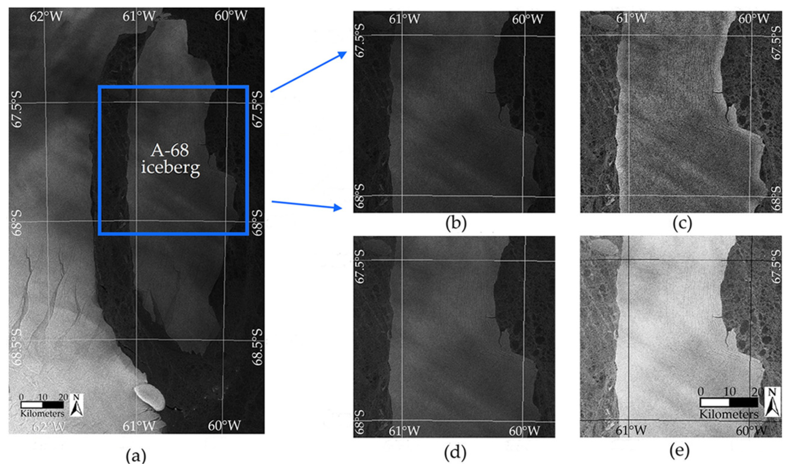
Using an experimental criterion, the Fuzzy parameter q was fixed at 0.6, but acceptable results are also obtained with , and in this case, the histogram information is distributed in the middle range. Grey tones are shifted to the right when a low q value is assigned, producing an overexposed look. In order to evaluate its performance, the applied Fuzzy algorithm was compared with alternative contrast solutions: (a) the contrast limited adaptive histogram equalization (CLAHE) [30], and (b) the exponential grey-scale transformation. The SAR image with an acquisition date of 13 December 2017 was selected as the test image, as it displays a deficient contrast. Figure 2 shows: (a) The full input SAR image; (b) A selected window of 700 × 700 pixels of the input image; (c) Result of the CLAHE algorithm; (d) The exponential grey-scale transformation, and (e) Result of the applied Fuzzy algorithm. The fuzzifier parameter was fixed to . It is observed in (c) and (d) a regular distribution of the contrast. Both open-sea and non-open-sea elements are ambiguous regions and cannot be precisely defined even by visual inspection. The results are therefore unsatisfactory for a subsequent segmentation stage. In (e), the dark regions are slightly brighter, and the bright regions are brighter as well. The Fuzzy function maps the input image to a grey-level transformation, in agreement with the visual perception of contrast. Hence, the contrast of the sea-ice elements is enhanced.

Figure 2.
Comparison of contrast enhancement algorithms: (a): Overview of the input SAR image of 13 December 2017; (b): Window of the SAR input image; (c): Result of the CLAHE algorithm; (d): The exponential grey-scale transformation, and (e): Result of the applied fuzzy algorithm. This algorithm improves the dark and bright feature contrast. As a result, the mapping of the grey level range enhances the discrimination of the iceberg structure.
4.2. Stochastic Segmentation
The energy term requires the mean and variance of the Gaussian modes. The set of parameters was obtained by manually training windows over the observed ice sheet and non-ice sheet regions. In terms of the Ising model, the parameters of Equation (5), were fixed to , and . The variables and are the one-site clique and the two-site cliques, respectively. The parameters , M and were fixed by experimental evidence. A modest contribution is expected by the pixel-based analysis and, for this reason, the information of the site was given using and a M value equal to 1. The parameter is important because produces under segmentation, while over segmentation. Thus, an appropriate domain is . The simulated annealing process requires a numerical simulation. During the iterative process, we compute the pixel difference between adjacent sampled images. At iteration 40, the attained rate of change is about 0.077%. Hence, after 40 iterations, the algorithm reaches the convergence. The derived variance of the A-68A grey level ranges from 100 to 400, which implies a transformation of the pixel region process. Consequently, an overlap is observed between the modes of the intensity histogram, and this is a basic problem in SAR image segmentation. To tackle this problem, a contextual second-order neighbourhood model and the Ising model are needed for MRF segmentation.
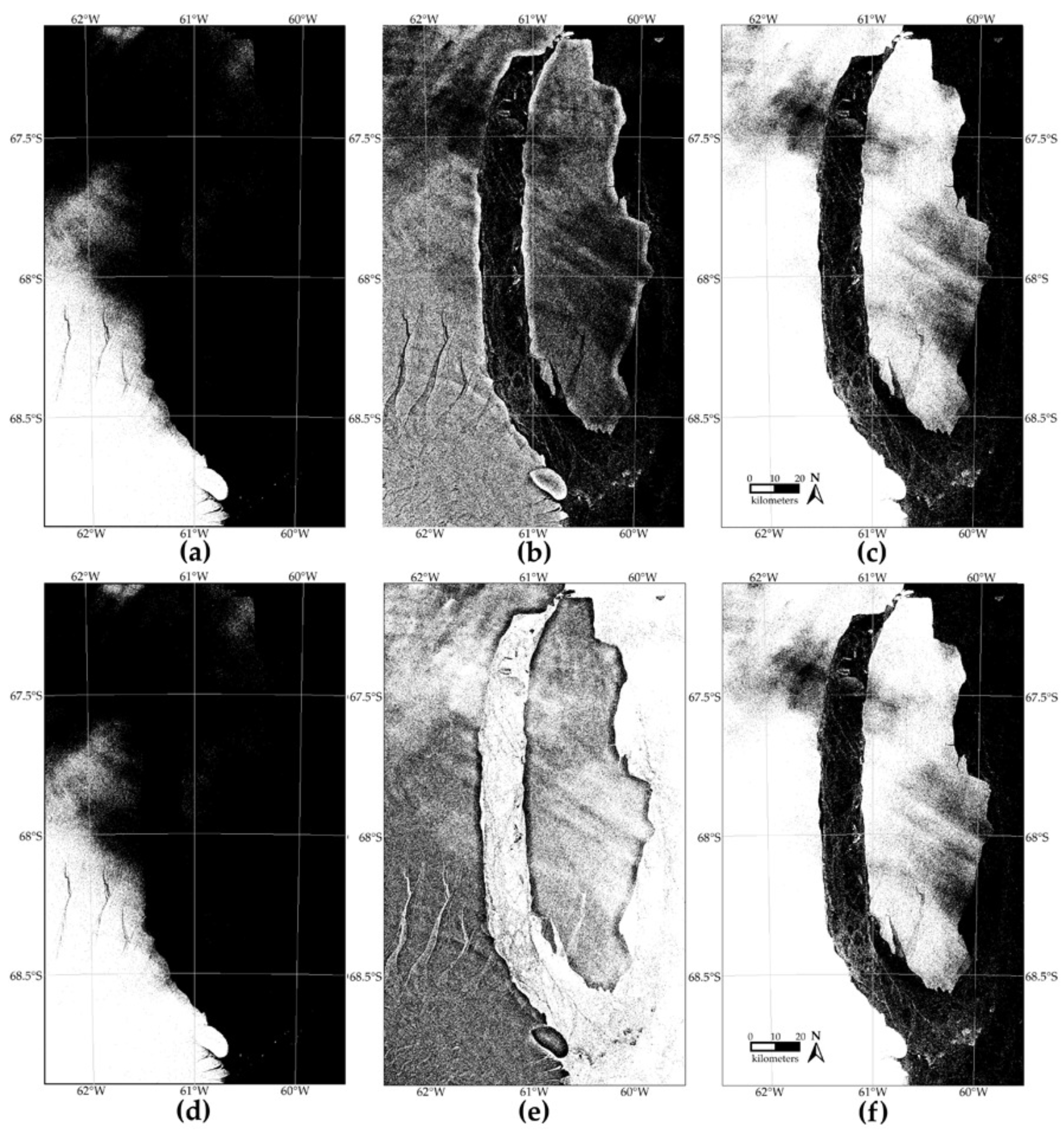
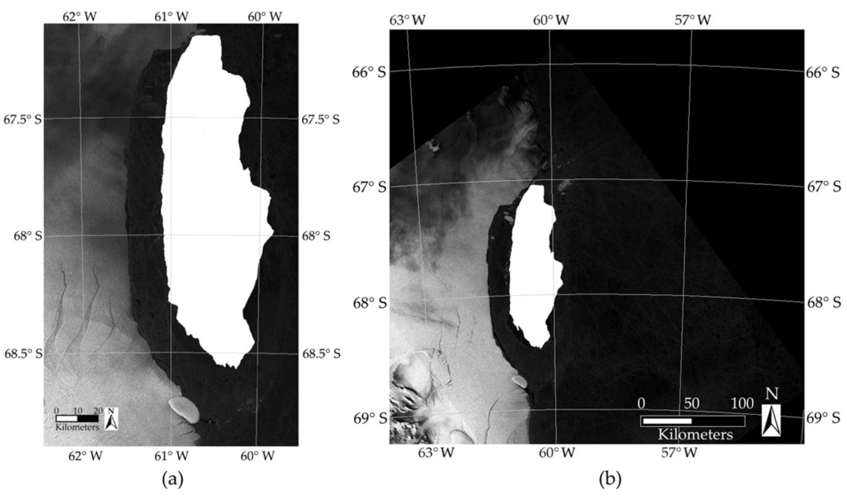
The k-means and Fuzzy c-means (FCM) algorithms were the reference ones to evaluate the effect of the contrast enhancement algorithm on the binary segmentation stage. They are based on iterative cost function optimization and are well known in pattern recognition applications. The image of 13 December 2017, see Figure 2, was the test image. Using as input images the exponential grey-scale transformation, the CLAHE, and the proposed Fuzzy solution, respectively, Figure 3a–c show the k-means segmentation results, while Figure 3d–f show the FCM segmentation results. It is observed: (i) that noisy segmentation patterns are obtained when the CLAHE and the exponential grey-scale transformation are the input images; and (ii) these results can hardly be used for performing the iceberg detection task, but improved segmentation is observed when applying the Fuzzy contrast enhancement algorithm as a preprocessing step; see Figure 3c,f. Using the proposed stochastic scheme, Figure 4a shows the iceberg detection of the image of 13 December 2017, while Figure 4b shows the corresponding result for 18 January 2018. The Fuzzy contrast enhancement operation (see Section 3.2) was the preprocessing step. The detected iceberg shape is displayed in white, and for a better visualization, the whole SAR scenes are used.
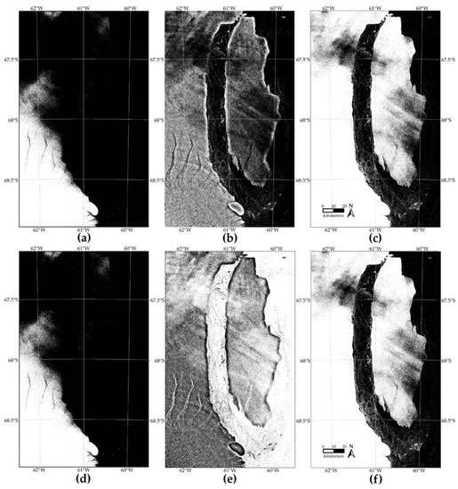
Figure 3.
Effect of the contrast enhancement algorithm on the segmentation stage. The applied fuzzy algorithm was compared with alternative contrast enhancement solutions (see Section 4.1) using two pixel-based segmentation algorithms. The image of 13 December 2017 is the test image. First case: the k-means segmentation results, where the input images were (a) the exponential grey-scale transformation, (b) the CLAHE, and (c) the proposed Fuzzy solution. Second case: the FCM segmentation results derived from (d) the exponential grey-scale transformation, (e) the CLAHE, and (f) the proposed Fuzzy solution. These are impractical results for performing the iceberg detection task, but, as can be seen in (c,f), an improved segmentation is observed using the Fuzzy contrast enhancement algorithm as a preprocessing step.

Figure 4.
Segmentation results obtained by the proposed scheme: (a) Image of 13 December 2017, and (b) Image of 18 January 2018. The detected A-68A object is displayed in the input SAR scenes. The detected shape is homogeneous and without spurious pixels.
4.3. Measurement of the Drift Trajectory
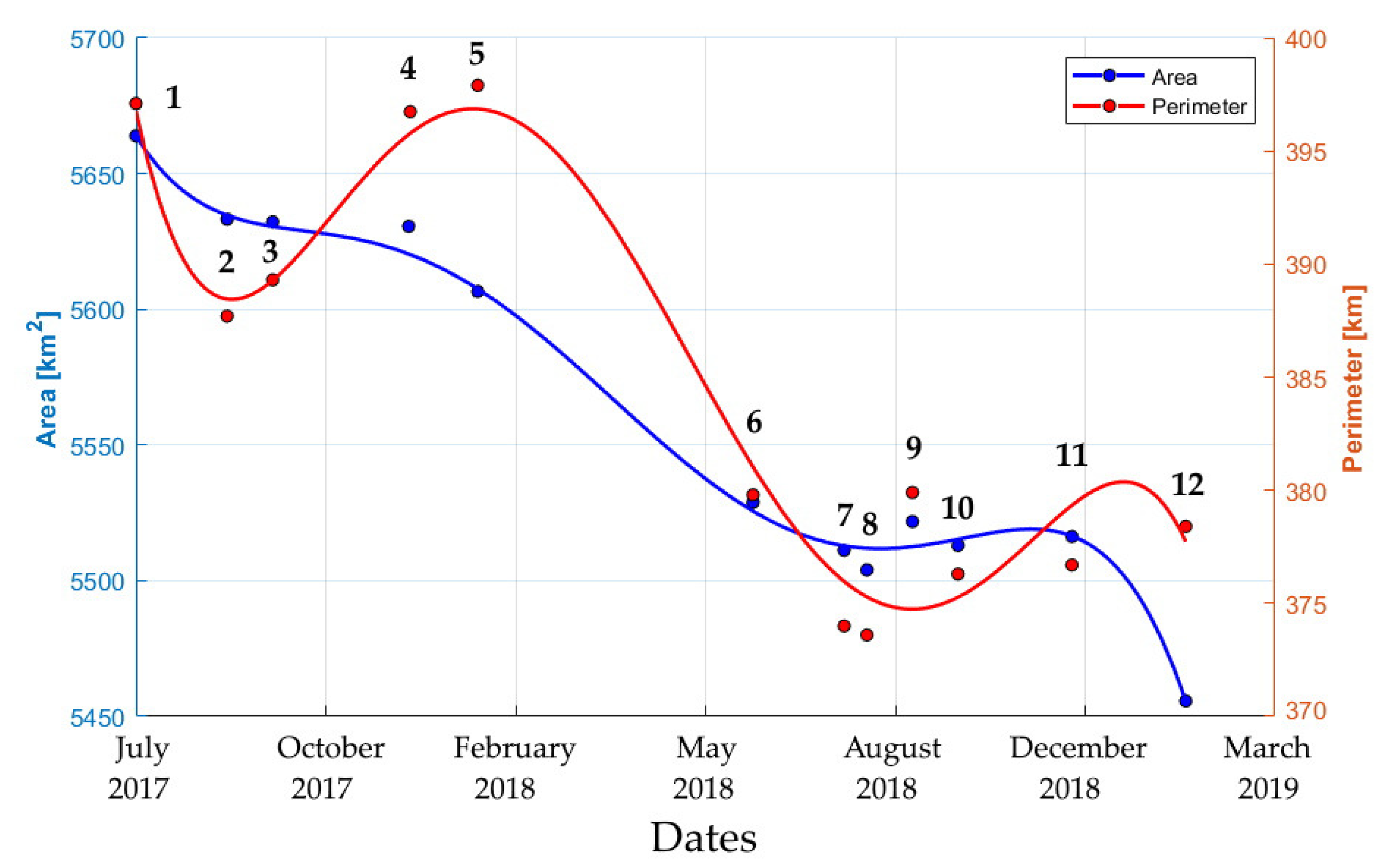
Based on the segmentation result, the objects of the binary field are labelled, and the iceberg shape can be detected and extracted from the input images. Computation of its geometric parameters is now a straightforward task. By geometric properties, the pixels of the iceberg form are described by ellipse parameters. The connected components are specified as pixel structures, and by statistical moments, a set of properties can be derived from the labelled iceberg form. The first central moment is the geometric centre of the plane form (the centroid). The second central moments of an equivalent ellipse are the basis for computing the covariance matrix, whose eigenvectors relate to the major and minor axes of the iceberg form. For each input image, the retrieved parameters were: area, perimeter and coordinates of the centroid. For the analyzed period, the image acquisition dates were (1): 22 July 2017, (2): 8 August 2017, (3): 2 October 2017, (4): 13 December 2017, (5): 18 January 2018, (6): 12 June 2018, (7): 30 July 2018, (8): 11 August 2018, (9): 4 September 2018, (10): 28 September 2018, (11): 27 November 2018 and (12): 26 January 2019. Figure 5 shows the variation of the area on the left of the y-axis and the perimeter on the right of the y-axis. To appreciate the long-term tendency, a curve fitting function was used: for both parameters, a 5th-degree polynomial curve fits the series of data points. A decay tendency is observed in both area (blue curve) and perimeter (red curve) parameters.
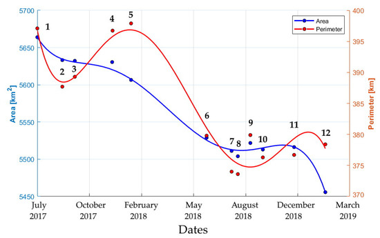
Figure 5.
The derived time-series data of the A-68A iceberg. Based on a polynomial least squares regression, the blue and red curves display the long-term tendency of the area and perimeter parameters. The analysis does not take into account the A-68B iceberg.
We point out the proportional relationship between perimeter and area, of which the rate reveals a steady behaviour. For example, for the first and the last image, the rate perimeter/area is 0.0694 and 0.0701, respectively. For the image sequence, the mean rate is 0.0689.
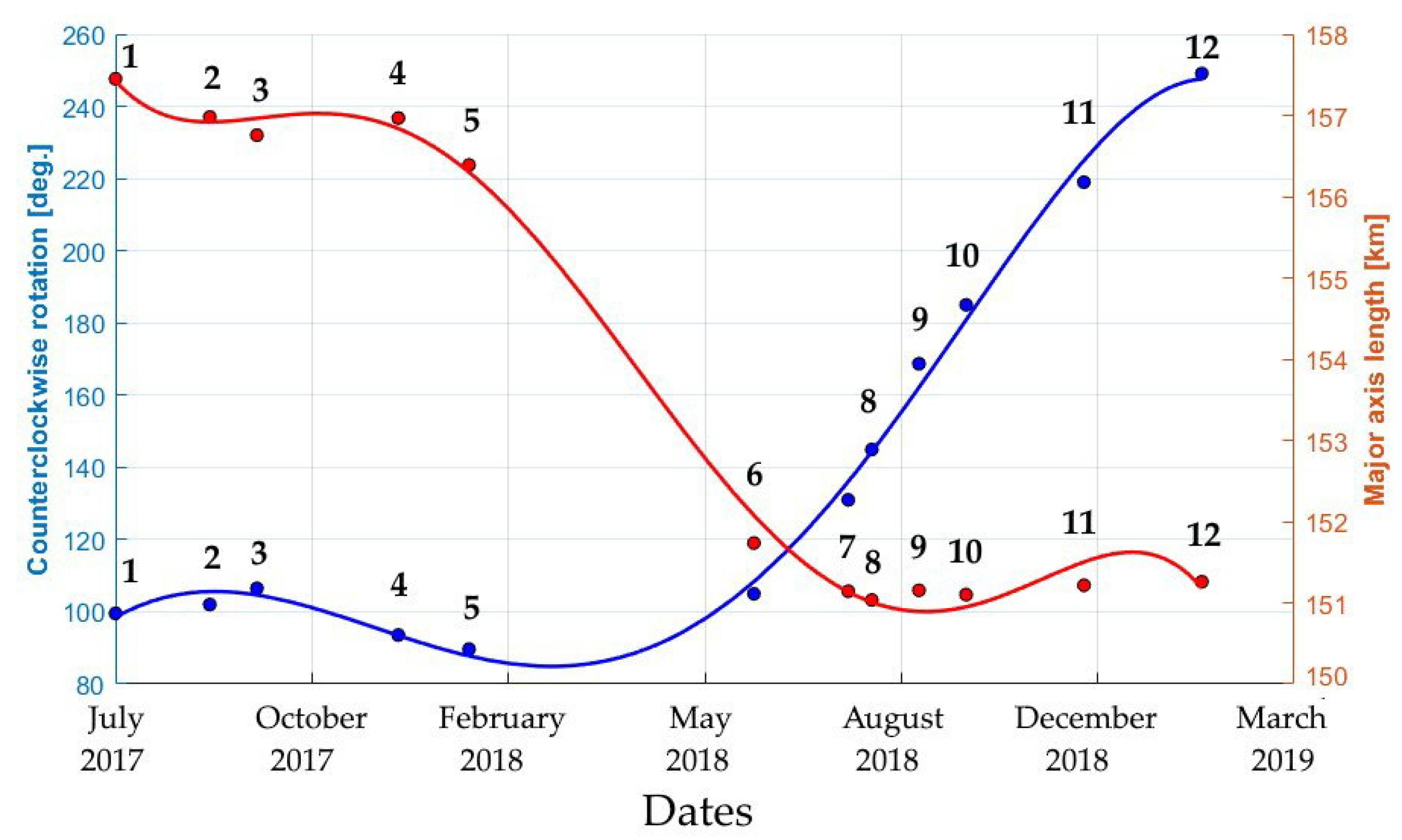
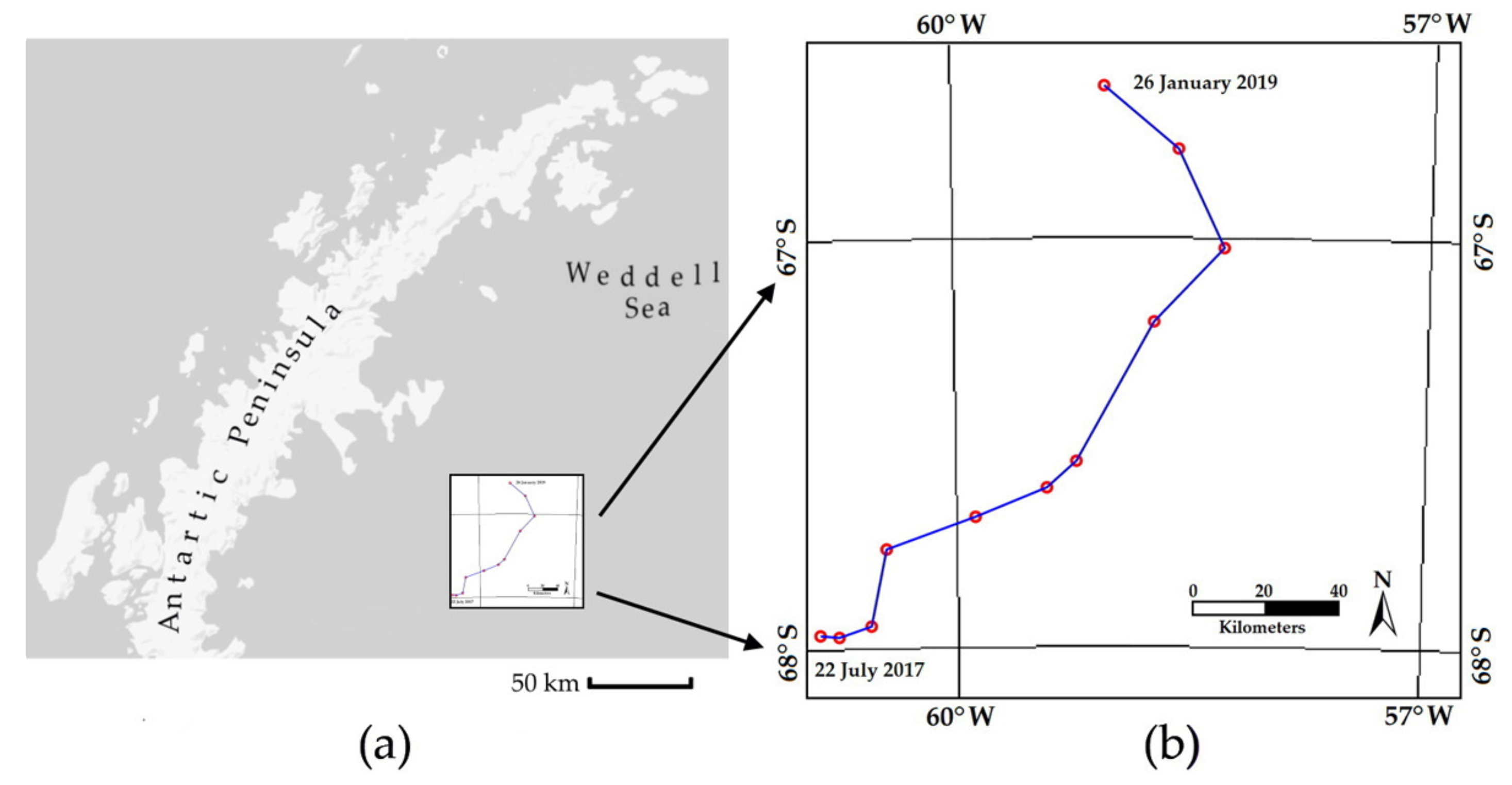
Two complementary parameters are the major axis length and the rotation angle. The geometric centroid (center of mass) of the connected iceberg pixels, i.e., concurrency point of both the major and minor axes, was derived. The two axes are marked as the segments AB and CD in Figure 1. Taking as reference the horizontal axis and the segment defined by the centroid and point A, the rotation angle is computed in a counter-clockwise sense. Figure 6 displays the rotation angles derived from the first and the last analysed images. During the year 2017, the iceberg remained near the collapse zone: the displacement was reduced by the surrounded sea ice and the seabed of Gipps Ice Rise. In the course of the first six months of 2018, the sea floor elevation layers of the Bawden Ice Rice affected the A-68A’s drift movement, and the iceberg remained almost static. In July 2018, due to southerly winds, it started a slow movement, remaining the north margin of the iceberg stuck in the shallow seabed of the Bawden Ice Rise region (about −300 m), and the iceberg turned around point A of Figure 6 in an anticlockwise direction. By August 2018, the rotation was about 160. Figure 7 shows the time evolution of both the rotation angle and the major axis length parameters. For a time period of 553 days, from 22 July 2017 to 26 January 2019, Figure 8 shows the estimated drift positions. The analysis does not take into account the A-68B iceberg.
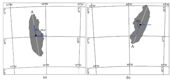
Figure 6.
The derived rotation angle of the A-68A iceberg: (a) Image of 22 July 2017, the initial angle was 99.6; (b) Image of 26 January 2019, the angle was 249.

Figure 7.
Angle and major axis length progression. Based on a polynomial least-squares regression, a 5th-degree polynomial curve fits the series of data points. The blue and red curves display the long-term tendency of rotation angle and major axis length.

Figure 8.
The derived sequence of the A-68A iceberg positions: (a) Overview of the derived iceberg drift, eastern Antarctic Peninsula (Google Maps©). The blue rectangle indicates the drift area; (b) Iceberg locations. The centroid coordinates are used to display the drift trajectory.
5. Discussion
The multiplicative nature of speckle degradation produces spurious pixel grey level values, and this statistical confusion is a basic difficulty for SAR image segmentation. To address the random nature of the SAR data, two probability abstractions provide the required information: a contextual second-order neighbourhood model and a pixel-based analysis. Therefore, the segmented field is the result of a double segmentation model which was implemented using numerical optimization. Two training windows are manually fixed to derive the mean values of the ice sheet and non-ice sheet objects. This is done for each image analyzed. Under-segmentation or over-segmentation is the result of an inappropriate selection of the mean values. The language used to implement the algorithms was MATLAB®. Using a laptop with Intel(R) Core(TM) i7-7700HQ, CPU @2.8GH and 8GB Ram, the CPU time was 1.26 seconds for the Fuzzy algorithm and 19.04 minutes for the stochastic segmentation. A trained person could perform manual tracing more quickly, but the goal of our method is to arrive at semi-automated detection. Figure 5 shows some increases in the time series area, but this can be attributed to the attachment of sea ice fragments. Because of the contextual analysis (to decide the class of a given pixel, its 8-neighbouring pixels are taken into account), the contours are detected with one-pixel position accuracy. Concerning the tracking application, see Figure 8, during the year 2017, the iceberg remained near the collapse zone: the displacement was only some 30 km towards the Eastern Weddell Sea, and the area was 99% intact. The sea-floor elevation layers of the Bawden Ice Rice affected A-68A’s drift movement and the iceberg did not move much during the first six months of 2018. In July 2018, it started to swing slowly in an anticlockwise direction. In the period July 2017 to August 2018, the computed mean speed was 7.2 km/month. By the end of September 2018, the rotation angle was 185 (see Figure 7, point 10), and the speed had increased to 16.8 km/month. By January 2019, the angle of the major axis was about 250. Using the centroid data, the total displacement distance was 220.6 km. In the analyzed period, a slight reduction in the planar shape parameters was observed. Perimeter and area are directly proportional parameters. The perimeter/area rate is steady, and for the image sequence, the mean rate is 0.0689. The visible iceberg area decreased by about 3.7% and the major axis length by 3.9%.
Melting, breakup and forced motion are consequences of the iceberg–environment interaction; the main driving force is the surrounding ocean with some atmospheric contributions. Large icebergs last for several years and the gravitational force may introduce topological changes. The gravitational force pushes the iceberg mass outward, and, over the years, the cumulative effect produces a decrease in thickness and an increase in iceberg length [31]. The influence of these elements is beyond the scope of this paper. In the last analyzed image, the A-68A iceberg was approaching the marginal zone of the Antarctic Circle. At this point, the coastal current is expected to be the driving force of its displacement. Moving in the direction of the Scotia Sea, the iceberg must still travel about 400 km to reach the most northerly point of the Antarctic Peninsula.
6. Conclusions
A methodology is proposed for the analysis of a temporal sequence of SAR images. Two fundamental problems in the remote sensing domain are irregular image contrast and mixed multimodal class distribution. This paper takes image uncertainty into account by proposing the combined use of fuzzy logic and of a ferromagnetic approach which models overlapping class intervals. A preprocessing stage implements a fuzzy contrast enhancement in the spatial domain. In the fuzzification process, a set of image features define the membership functions whose domain and range are a rough fit to the image feature histogram. The concepts of ferromagnetic theory were chosen to define a stochastic segmentation method. In ferromagnetic theory, the effect of an external magnetic field is to induce alignment of the ferromagnetic elements; in the case of a segmentation process, this simulates the magnetic attractive force by generating local homogeneous pixel configurations. The Ising model and the Bayes equation were the basis for implementing the spatial pixel interaction. The derived binary field is the result of a stochastic minimization process. Due to the size of the scene and the recursive nature of the optimization algorithm, the computational load of MRF segmentation is intense. The final analysis shows the movement of the A-68A iceberg over a time period. Due to its colossal size, small variations in area, perimeter and major axis length parameters were observed. Up to 26 January 2019, the detected area was 96% of its original size. The surrounding ice in the winter season, wind patterns and sea floor elevation layers cause irregular displacements and varying iceberg velocities, but the dominant direction seems to be towards the Eastern Weddell Sea. The main contribution of this paper is in the image processing domain applied to the tracking or path visualisation of the A-68A iceberg. Ancillary information such as meteorological data, ocean currents, wind speed, temperature and geomorphology of the seabed was not available for this study, but the proposed methodology can be integrated to perform dynamic modelling.
Author Contributions
Conceptualization, L.L.-L., F.P., M.M.-F. and L.G.; Methodology, L.L.-L. and M.M.-F.; Validation, L.L.-L.; Formal analysis, L.L.-L. and M.M.-F.; Data curation, L.G.; Writing—original draft preparation, L.L.-L., F.P., M.M.-F. and L.G.; Writing—review and editing, L.L.-L., F.P., M.M.-F. and L.G.; Visualization, L.L.-L., F.P., M.M.-F. and L.G.; Supervision, F.P. All authors have read and agreed to the published version of the manuscript.
Funding
This research was partially funded by Universidad Nacional Autónoma de México and Consejo Nacional de Ciencia y Tecnología through scholarship grant number 099598462.
Institutional Review Board Statement
Not applicable.
Informed Consent Statement
Not applicable.
Data Availability Statement
Not applicable.
Acknowledgments
The authors wish to thank the ESA Copernicus Program for making available the Sentinel-1 images through the open Scientific Data Hub.
Conflicts of Interest
The authors declare no conflict of interest.
Abbreviations
The following abbreviations are used in this manuscript:
| ESA | European Space Agency |
| CNR | National Research Council |
| CDMX | Mexico City |
| EW GRD | Extra Wide Swath Ground Range Detected |
| INGV | National Institute of Geophysics and Volcanology |
| USNIC | United States National Ice Center |
| MRF | Markov random field |
| UNAM | National Autonomous University of Mexico |
| SAR | Synthetic aperture radar |
| S1 EW GRD | Sentinel-1 Extra Wide Swath Ground Range Detected |
| T1 FSs | Type-1 Fuzzy Sets |
| T2 FSs | Type-2 Fuzzy Sets |
References
- Mazur, A.K.; Wåhlin, A.K.; Krężel, A. An object-based sar image iceberg detection algorithm applied to the amundsen sea. Remote Sens. Environ. 2017, 189, 67–83. [Google Scholar] [CrossRef]
- Tournadre, J.; Bouhier, N.; Girard-Ardhuin, F.; Rémy, F. Antarctic icebergs distributions 1992–2014. J. Geophys. Res. Ocean. 2016, 121, 327–349. [Google Scholar] [CrossRef]
- Scheick, J.; Enderlin, E.M.; Hamilton, G. Semi-automated open water iceberg detection from landsat applied to disko bay, west greenland. J. Glaciol. 2019, 65, 468–480. [Google Scholar] [CrossRef] [PubMed]
- Han, H.; Lee, S.; Kim, J.I.; Kim, S.H.; Kim, H.C. Changes in a giant iceberg created from the collapse of the larsen c ice shelf, antarctic peninsula, derived from sentinel-1 and cryosat-2 data. Remote Sens. 2019, 11, 404. [Google Scholar] [CrossRef]
- Meier, W.N.; Thorsten, M. Remote Sensing of Sea Ice; John Wiley & Sons, Ltd.: Hoboken, NJ, USA, 2014. [Google Scholar] [CrossRef]
- Zakhvatkina, N.; Vladimir, S.; Irina, B. Satellite sar data-based sea ice classification: An overview. Geosciences 2019, 9, 152. [Google Scholar] [CrossRef]
- Leira, F.S.; Johansen, T.A.; Fossen, T.I. A uav ice tracking framework for autonomous sea ice management. In Proceedings of the 2017 International Conference on Unmanned Aircraft Systems (ICUAS), Miami, FL, USA, 13–16 June 2017; pp. 581–590. [Google Scholar] [CrossRef]
- Yulmetov, R.; Aleksey, M.; Sveinung, L. Iceberg and sea ice drift tracking and analysis off north-east greenland. Ocean. Eng. 2016, 123, 223–237. [Google Scholar] [CrossRef]
- Demchev, D.; Volkov, V.; Kazakov, E.; Alcantarilla, P.F.; Sandven, S.; Khmeleva, V. Sea ice drift tracking from sequential sar images using accelerated-kaze features. IEEE Trans. Geosci. Remote Sens. 2017, 55, 5174–5184. [Google Scholar] [CrossRef]
- Muckenhuber, S.; Korosov, A.A.; Sandven, S. Open-source feature-tracking algorithm for sea ice drift retrieval from sentinel-1 sar imagery. Cryosphere 2016, 10, 913–925. [Google Scholar] [CrossRef]
- Collares, L.L.; Mauricio, M.M.; Rodrigo, K.; Jorge, A.-N.; Mauro, M.B. Iceberg drift and ocean circulation in the northwestern weddell sea, antarctica. Deep. Sea Res. Part II Top. Stud. Oceanogr. 2018, 149, 10–24. [Google Scholar] [CrossRef]
- Wesche, C.; Wolfgang, D. Estimating iceberg paths using a wind-driven drift model. Cold Reg. Sci. Technol. 2016, 125, 31–39. [Google Scholar] [CrossRef]
- Diansky, N.A.; Marchenko, A.V.; Panasenkova, I.I.; Fomin, V.V. Modeling iceberg drift in the barents sea from field data. Russ. Meteorol. Hydrol. 2018, 43, 313–322. [Google Scholar] [CrossRef]
- Andersson, L.E.; Francesco, S.; Lars, I. An estimation-forecast set-up for iceberg drift prediction. Cold Reg. Sci. Technol. 2016, 131, 88–107. [Google Scholar] [CrossRef]
- Bigg, G.R.; Cropper, T.E.; Clare, K.; O’Neill, A.K.; Arnold, A.H.; Fleming, R.M.; Ivchenko, V.; Nicolas, F.; Mike, O.; Robin, S. A model for assessing iceberg hazard. Nat. Hazards 2018, 92, 1113–1136. [Google Scholar] [CrossRef]
- Maître, H. (Ed.) Processing of Synthetic Aperture Radar Images; John Wiley & Sons, Ltd.: Hoboken, NJ, USA, 2010. [Google Scholar] [CrossRef]
- Leberl, F.W. Radargrammetric Image Processing; Artech House Remote Sensing Library; Artech House: Norwood, MA, USA, 1990. [Google Scholar]
- Xu, X.; Camilla, B.; Anthony, P.D.; Frank, M. Numerical analysis of microwave scattering from layered sea ice based on the finite element method. Remote. Sens. 2018, 10, 1332. [Google Scholar] [CrossRef]
- Richards, J.A. Remote Sensing with Imaging Radar; Springer: Berlin/Heidelberg, Germany, 2009. [Google Scholar] [CrossRef]
- Solomon, C.; Toby, B. Fundamentals of Digital Image Processing: A Practical Approach with Examples in Matlab, 1st ed.; Wiley Publishing: Hoboken, NJ, USA, 2011. [Google Scholar] [CrossRef]
- Nachtegael, M.; Van der Dietrich, W.; Etienne, K.; Van De Dimitri, V. Fuzzy Filters for Image Processing; Springer: Berlin/Heidelberg, Germany, 2003; Volume 122. [Google Scholar] [CrossRef]
- Kamel, M.; Aurélio, C. (Eds.) Type-2 Fuzzy Image Enhancement; Springer: Berlin/Heidelberg, Germany, 2005. [Google Scholar] [CrossRef]
- Pratt, W.K. Digital Image Processing: PIKS Inside, 3rd ed.; John Wiley & Sons, Inc.: New York, NY, USA, 2001. [Google Scholar] [CrossRef]
- Mendel, J.M. Type-2 fuzzy sets and systems: An overview. IEEE Comput. Intell. Mag. 2007, 2, 20–29. [Google Scholar] [CrossRef]
- Tizhoosh, H.R. Image thresholding using type ii fuzzy sets. Pattern Recognit. 2005, 38, 2363–2372. [Google Scholar] [CrossRef]
- Chaira, T. Fuzzy Set and Its Extension: The Intuitionistic Fuzzy Set; John Wiley & Sons, Ltd.: Hoboken, NJ, USA, 2019. [Google Scholar] [CrossRef]
- Sigelle, M.; Ronfard, R. Modèles de potts et relaxation d’images de labels par champs de markov. Traitement du Signal 1992, 9, 449–458. [Google Scholar]
- Ibe, O. Markov Processes for Stochastic Modeling, 2nd ed.; Elsevier Insights; Elsevier Science: London, UK, 2013. [Google Scholar] [CrossRef]
- Chatelain, F.; Xavier, D.; Florent, L.; Christian, L.; Clement, M.; Robert, M.; Michel, S.; Marc, S.; Radu, S.; Elena, Z. Applications de la Géometrie Stochastique à L’analyse D’images; Hermes Science-Lavoisier: Paris, France, 2011. [Google Scholar]
- Zuiderveld, K. Viii.5.-contrast limited adaptive histogram equalization. Graph. Gems 1994, 474–485. [Google Scholar] [CrossRef]
- Bigg, G.R. Icebergs: Their Science and Links to Global Change; Cambridge University Press: Cambridge, UK, 2015. [Google Scholar] [CrossRef]
Publisher’s Note: MDPI stays neutral with regard to jurisdictional claims in published maps and institutional affiliations. |
© 2021 by the authors. Licensee MDPI, Basel, Switzerland. This article is an open access article distributed under the terms and conditions of the Creative Commons Attribution (CC BY) license (http://creativecommons.org/licenses/by/4.0/).


