
Single-Pass Soil Moisture Retrieval Using GNSS-R at L1 and L5 Bands: Results from Airborne Experiment

 ,
,  , , ,
, , ,  , ,
, ,  , and
, and 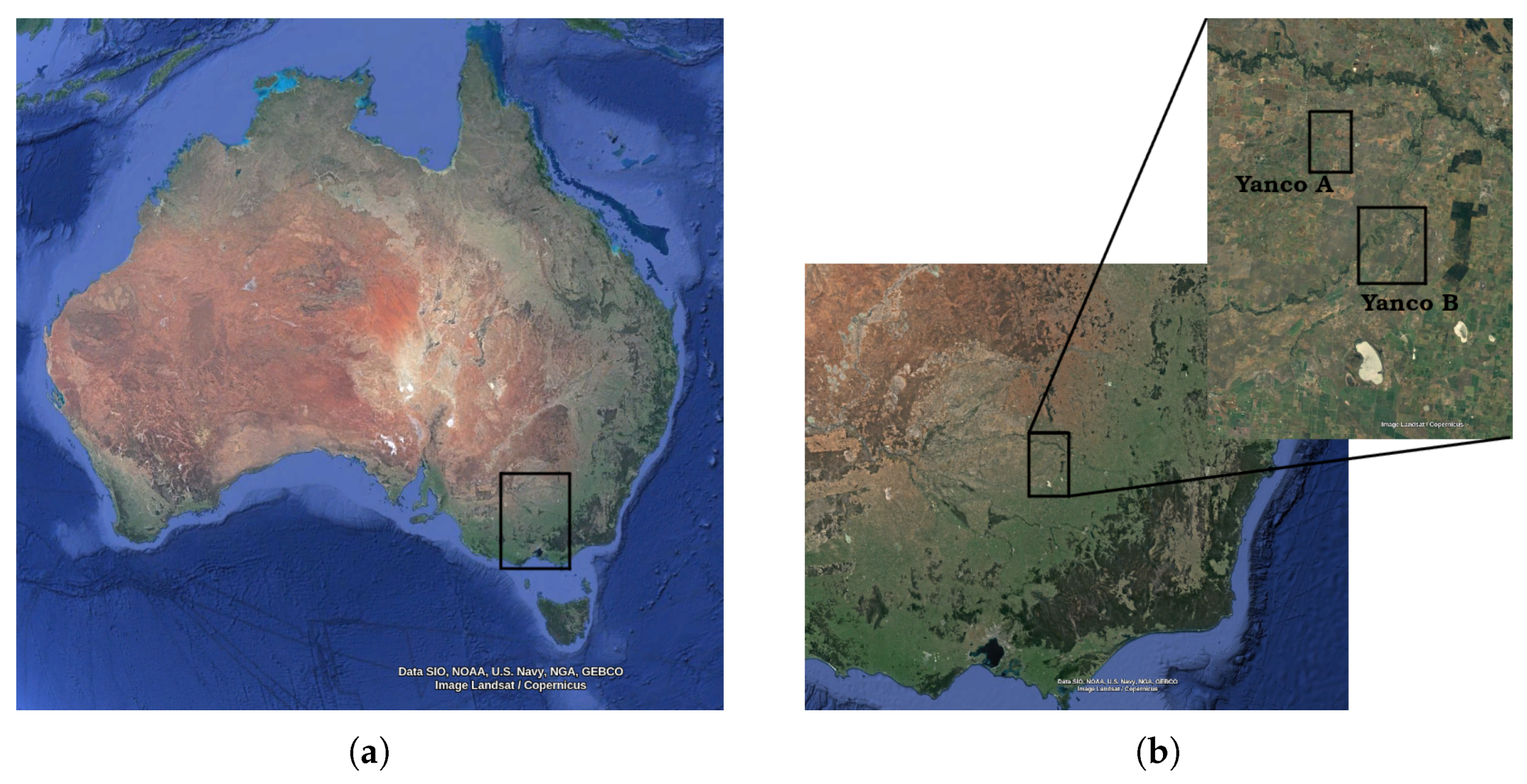
Abstract
1. Introduction
2. Data Description
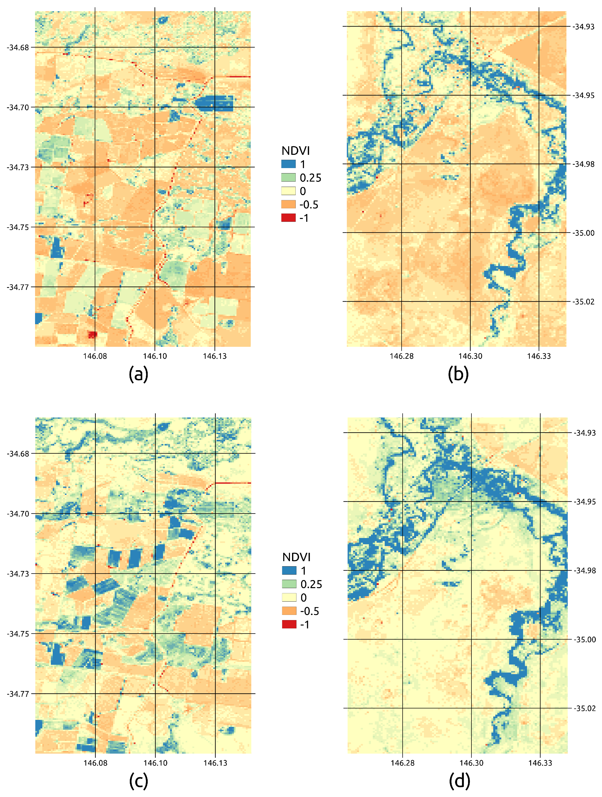
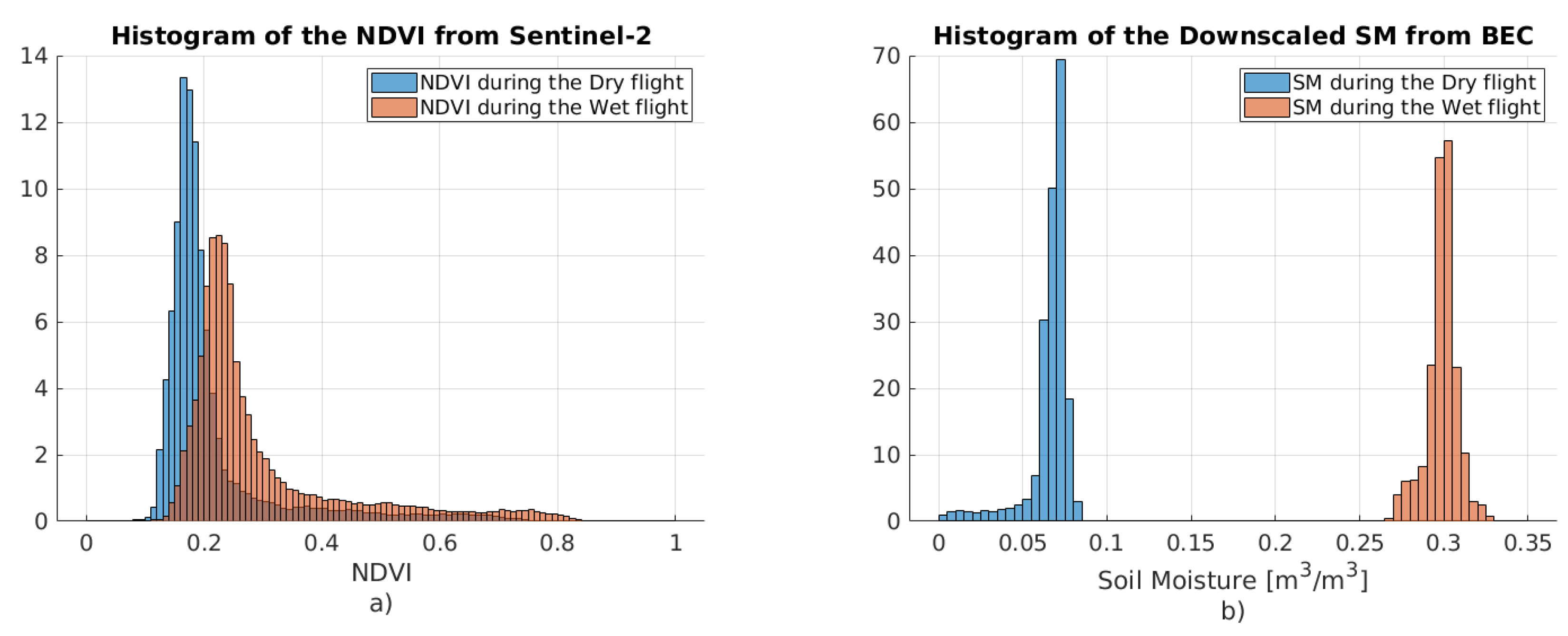
2.1. Ground-Truth and Ancillary Data
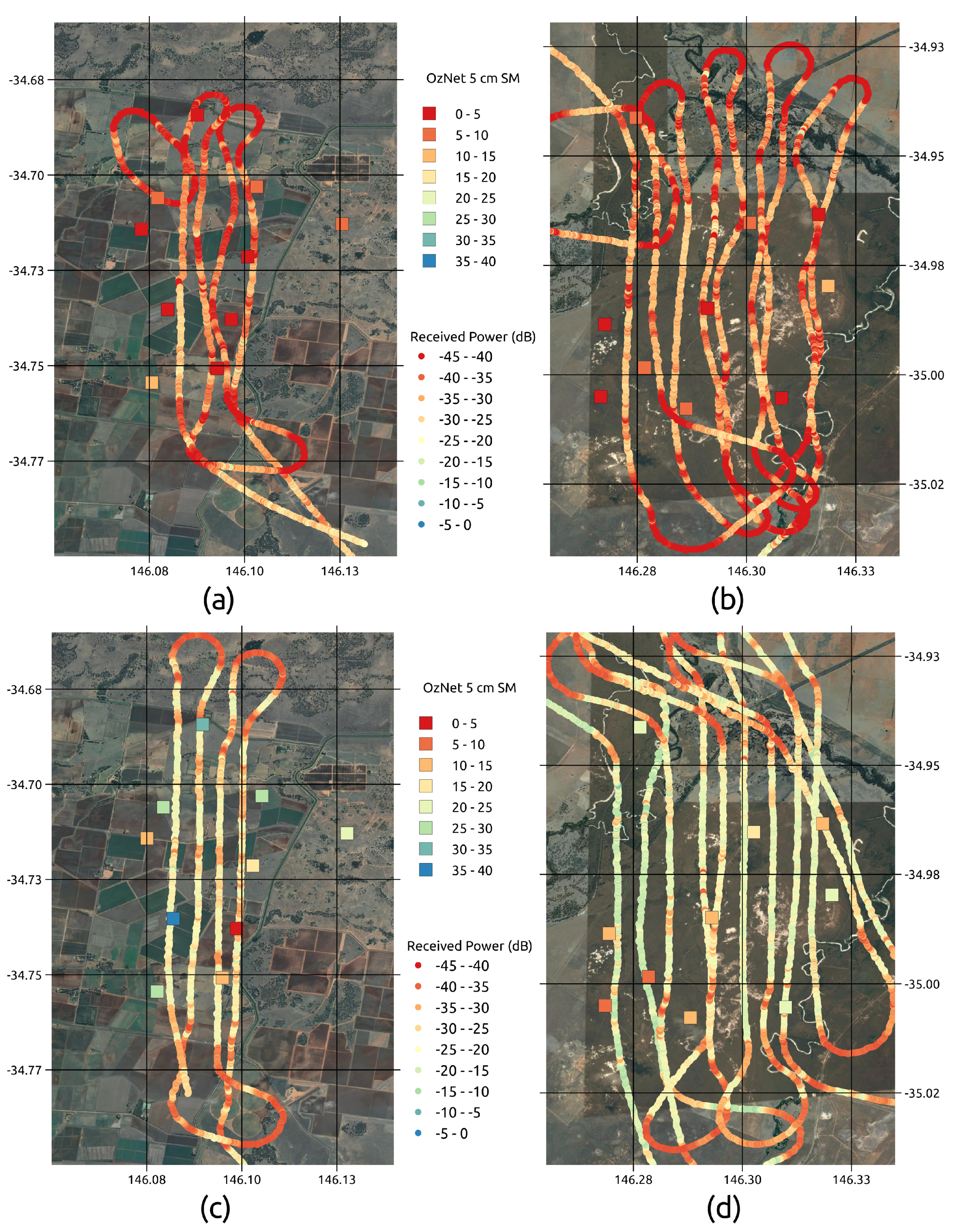
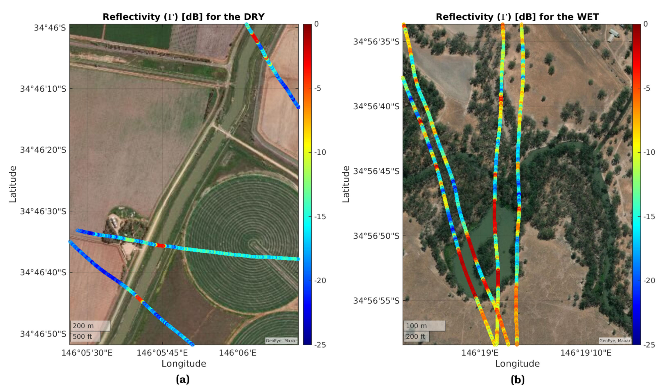
2.2. GNSS-R Data
3. Soil Moisture Retrieval Using GNSS-R
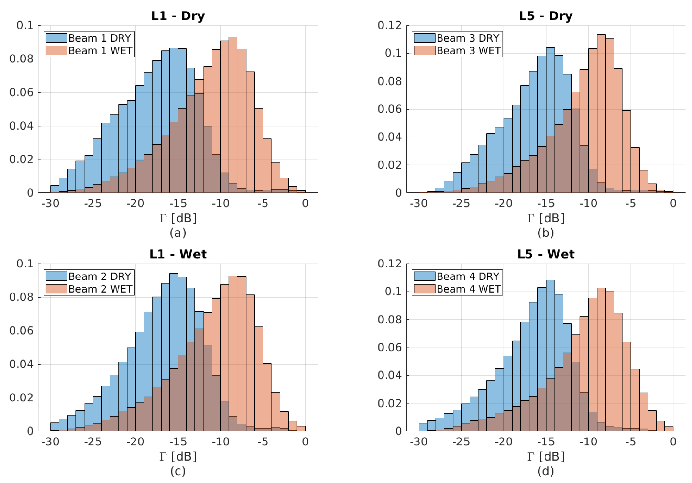
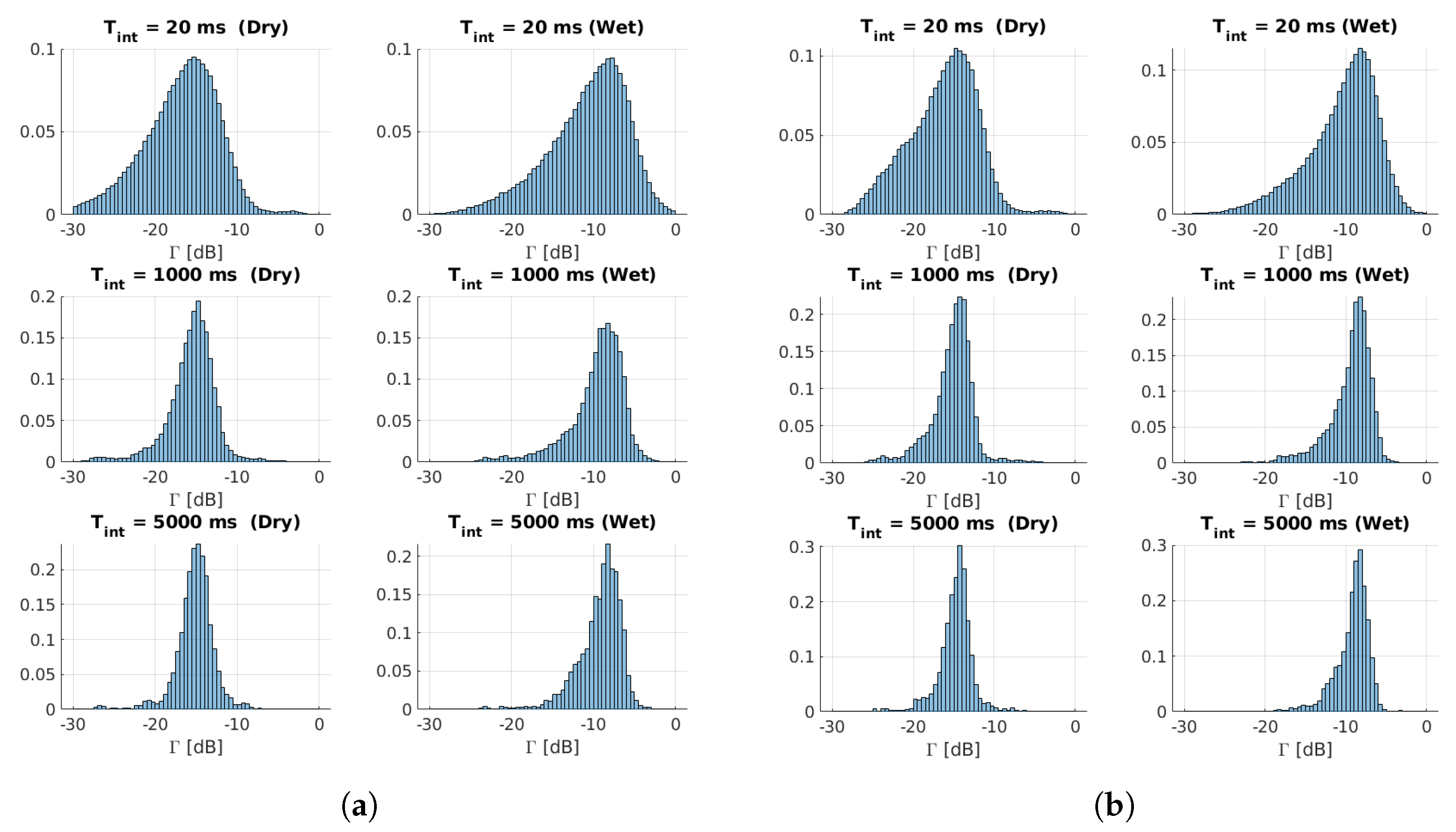
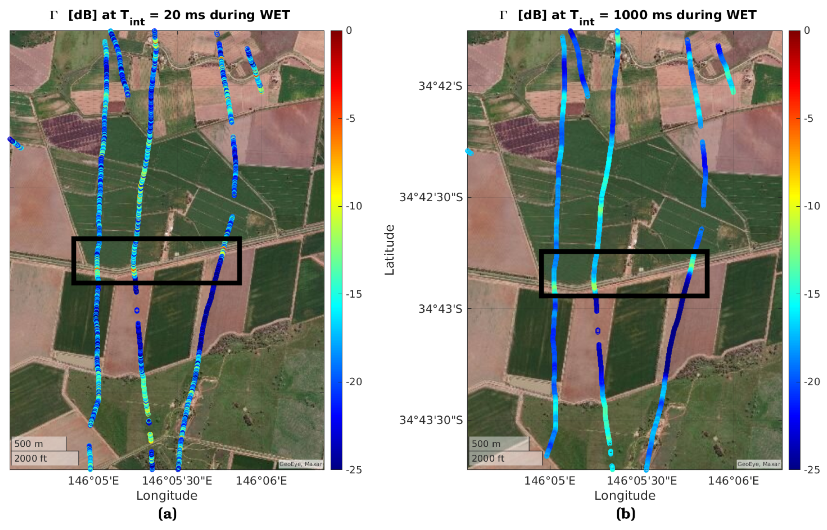
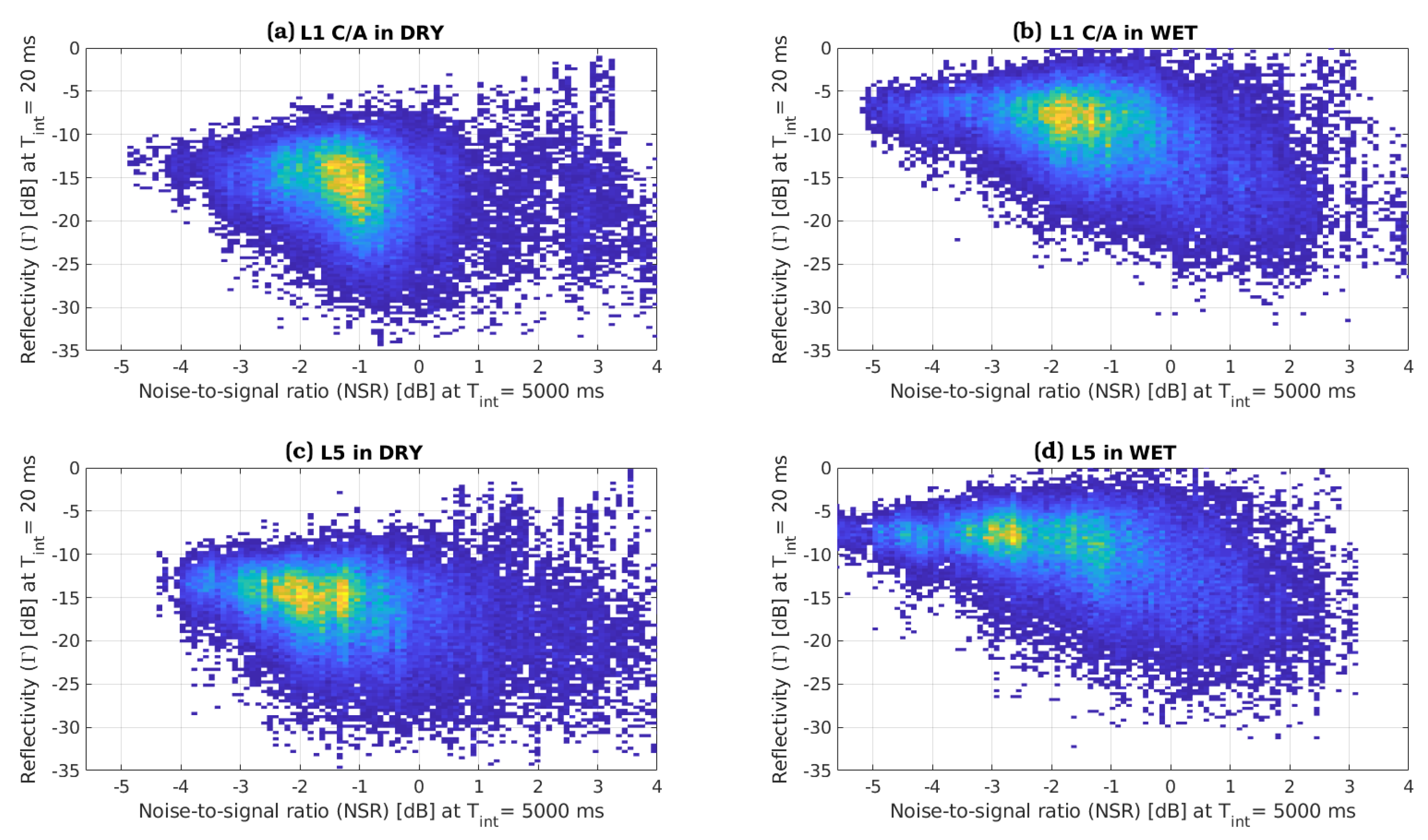
3.1. Reflectivity Statistics Using Different Integration Times
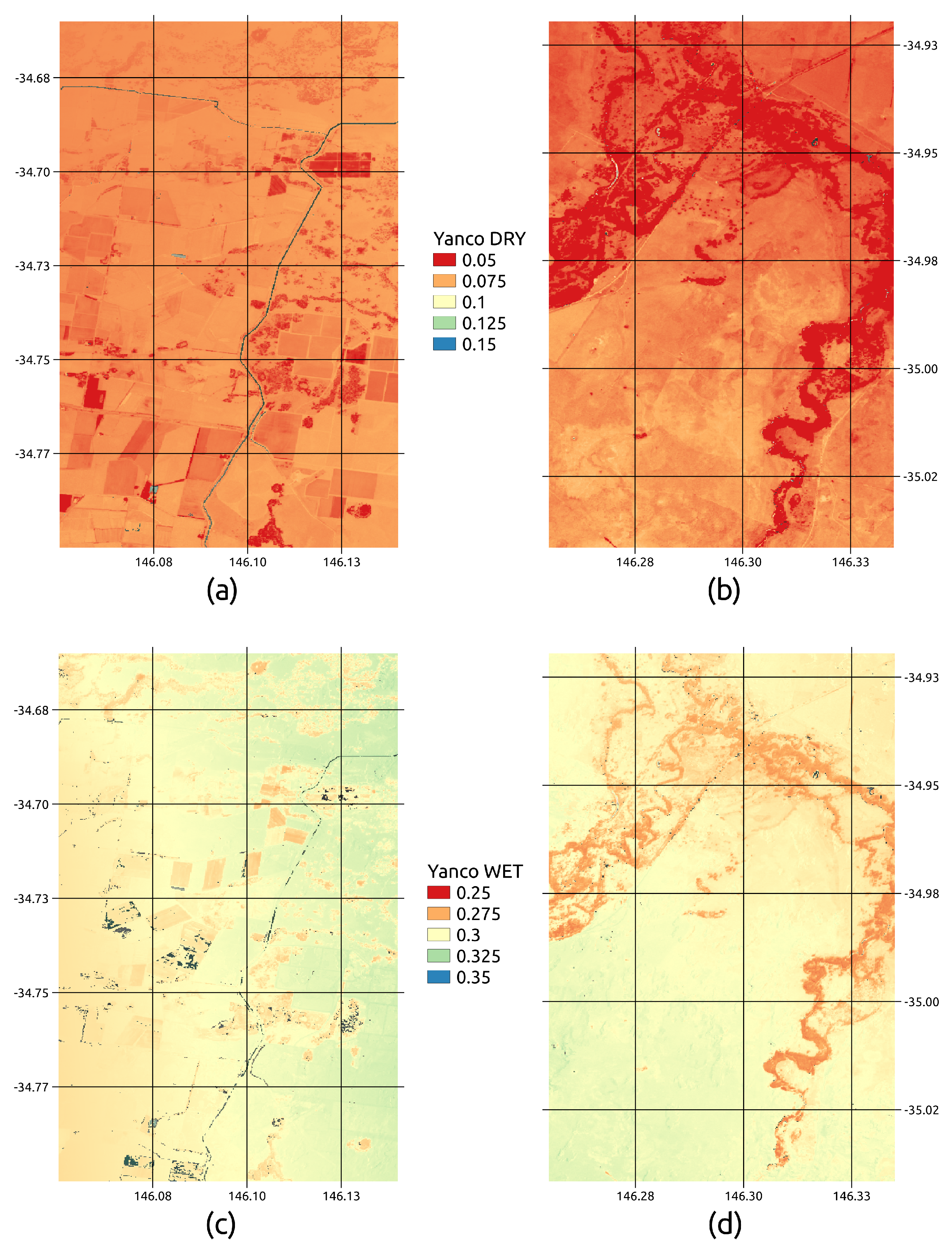
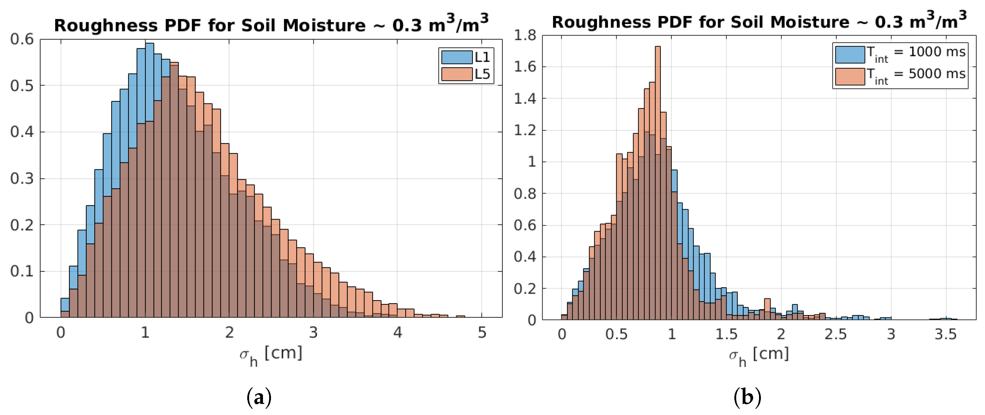
3.2. Surface Roughness Effect in Soil Moisture Retrievals
4. Soil Moisture Retrieval Algorithms
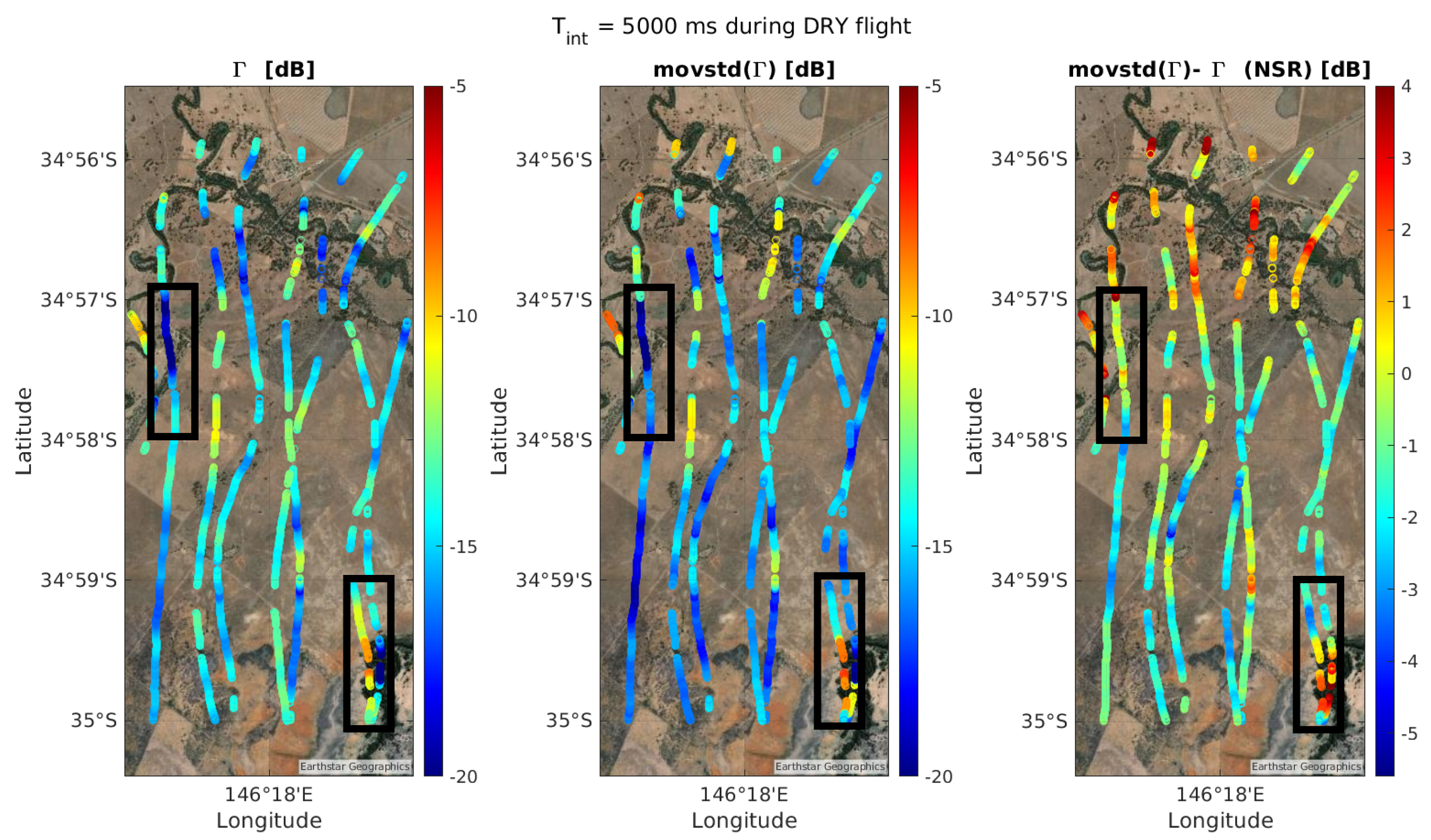
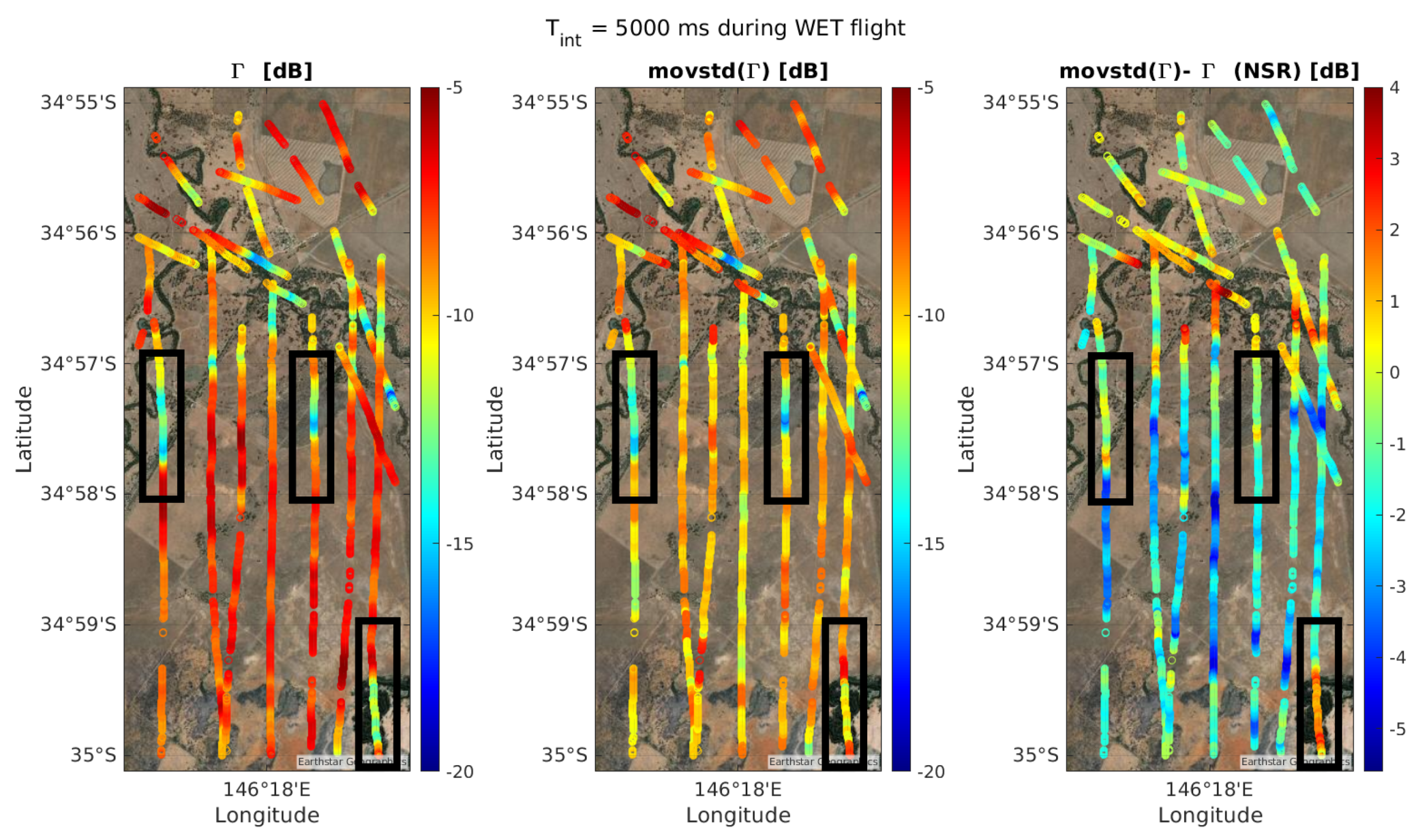
4.1. Surface Roughness and Reflectivity Standard Deviation
4.2. Artificial Neural Network
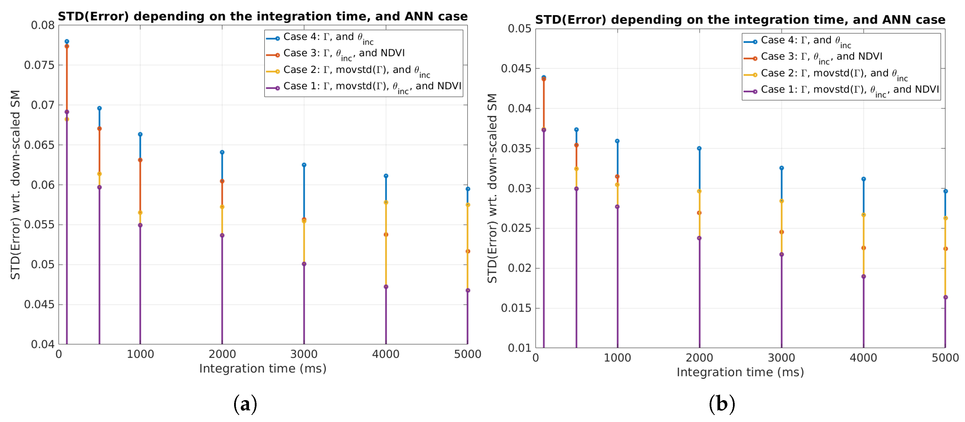
- (1)
- , movstd() as a proxy for , NDVI, and ,
- (2)
- , NDVI, and ,
- (3)
- , movstd() as a proxy for , and ,
- (4)
- , and .
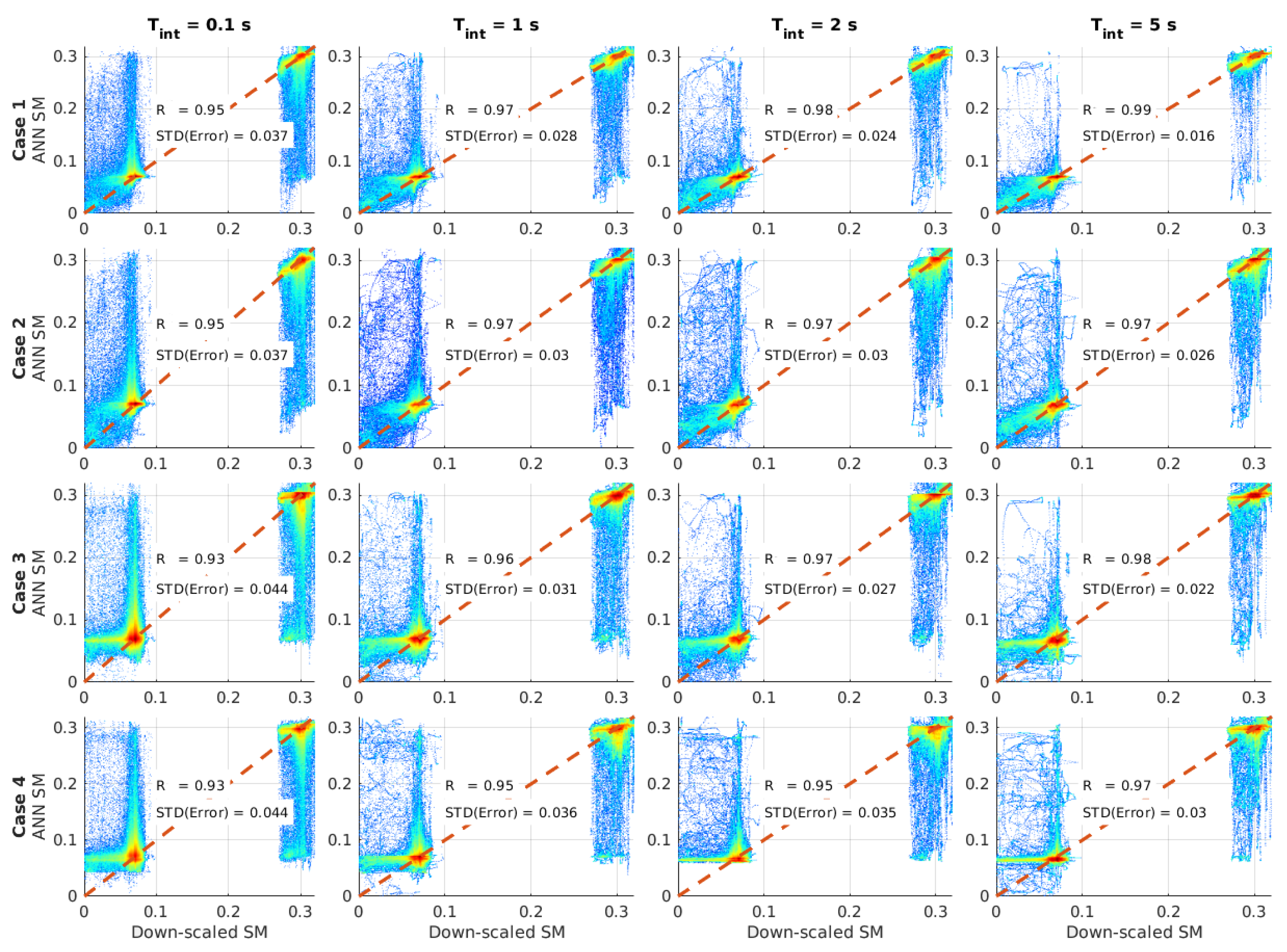
4.3. Results
4.4. Discussion
5. Conclusions
Author Contributions
Funding
Institutional Review Board Statement
Informed Consent Statement
Data Availability Statement
Acknowledgments
Conflicts of Interest
References
- Wasko, C.; Nathan, R. Influence of changes in rainfall and soil moisture on trends in flooding. J. Hydrol. 2019, 575, 432–441. [Google Scholar] [CrossRef]
- Wei, L.; Zhang, B.; Wang, M. Effects of antecedent soil moisture on runoff and soil erosion in alley cropping systems. Agric. Water Manag. 2007, 94, 54–62. [Google Scholar] [CrossRef]
- Miralles, D.G.; Gentine, P.; Seneviratne, S.I.; Teuling, A.J. Land-atmospheric feedbacks during droughts and heatwaves: State of the science and current challenges. Ann. N. Y. Acad. Sci. 2018, 1436, 19–35. [Google Scholar] [CrossRef] [PubMed]
- Kerr, Y.H.; Waldteufel, P.; Wigneron, J.P.; Delwart, S.; Cabot, F.; Boutin, J.; Escorihuela, M.J.; Font, J.; Reul, N.; Gruhier, C.; et al. The SMOS Mission: New Tool for Monitoring Key Elements ofthe Global Water Cycle. Proc. IEEE 2010, 98, 666–687. [Google Scholar] [CrossRef]
- Entekhabi, D.; Njoku, E.G.; ONeill, P.E.; Kellogg, K.H.; Crow, W.T.; Edelstein, W.N.; Entin, J.K.; Goodman, S.D.; Jackson, T.J.; Johnson, J.; et al. The Soil Moisture Active Passive (SMAP) Mission. Proc. IEEE 2010, 98, 704–716. [Google Scholar] [CrossRef]
- Array Systems Computing Inc. ATBD for SMOS Level 2 Soil Moisture Processor Development Continuation Project. Available online: https://earth.esa.int/documents/10174/1854519/SMOS_L2_SM_ATBD (accessed on 9 November 2020).
- O’Neill, P.; Bindlish, R.; Chan, S.; Chaubell, J.; Njoku, E.; Jackson, T. ATBD for Level 2 & 3 Soil Moisture (Passive)Data Products. Available online: https://smap.jpl.nasa.gov/system/internal_resources/details/original/484_L2_SM_P_ATBD_rev_F_final_Aug2020.pdf (accessed on 9 November 2020).
- Jackson, R.D. Soil Moisture Inferences from Thermal-Infrared Measurements of Vegetation Temperatures. IEEE Trans. Geosci. Remote Sens. 1982, GE-20, 282–286. [Google Scholar] [CrossRef]
- Naeimi, V.; Scipal, K.; Bartalis, Z.; Hasenauer, S.; Wagner, W. An Improved Soil Moisture Retrieval Algorithm for ERS and METOP Scatterometer Observations. IEEE Trans. Geosci. Remote Sens. 2009, 47, 1999–2013. [Google Scholar] [CrossRef]
- Srivastava, H.; Patel, P.; Sharma, Y.; Navalgund, R. Large-Area Soil Moisture Estimation Using Multi-Incidence-Angle RADARSAT-1 SAR Data. IEEE Trans. Geosci. Remote Sens. 2009, 47, 2528–2535. [Google Scholar] [CrossRef]
- Paloscia, S.; Pettinato, S.; Santi, E.; Notarnicola, C.; Pasolli, L.; Reppucci, A. Soil moisture mapping using Sentinel-1 images: Algorithm and preliminary validation. Remote Sens. Environ. 2013, 134, 234–248. [Google Scholar] [CrossRef]
- Gorrab, A.; Zribi, M.; Baghdadi, N.; Mougenot, B.; Fanise, P.; Chabaane, Z. Retrieval of Both Soil Moisture and Texture Using TerraSAR-X Images. Remote Sens. 2015, 7, 10098–10116. [Google Scholar] [CrossRef]
- Rodriguez-Alvarez, N.; Bosch-Lluis, X.; Camps, A.; Aguasca, A.; Vall-llossera, M.; Valencia, E.; Ramos-Perez, I.; Park, H. Review of crop growth and soil moisture monitoring from a ground-based instrument implementing the Interference Pattern GNSS-R Technique. Radio Sci. 2011, 46. [Google Scholar] [CrossRef]
- Yin, C.; Lopez-Baeza, E.; Martin-Neira, M.; Fernandez-Moran, R.; Yang, L.; Navarro-Camba, E.A.; Egido, A.; Mollfulleda, A.; Li, W.; Cao, Y.; et al. Intercomparison of Soil Moisture Retrieved from GNSS-R and from Passive L-Band Radiometry at the Valencia Anchor Station. Sensors 2019, 19, 1900. [Google Scholar] [CrossRef]
- Alonso-Arroyo, A.; Camps, A.; Monerris, A.; Rudiger, C.; Walker, J.P.; Forte, G.; Pascual, D.; Park, H.; Onrubia, R. The light airborne reflectometer for GNSS-R observations (LARGO) instrument: Initial results from airborne and Rover field campaigns. In Proceedings of the 2014 IEEE Geoscience and Remote Sensing Symposium, Quebec City, QC, Canada, 13–18 July 2014; pp. 4054–4057. [Google Scholar] [CrossRef]
- Egido, A.; Paloscia, S.; Motte, E.; Guerriero, L.; Pierdicca, N.; Caparrini, M.; Santi, E.; Fontanelli, G.; Floury, N. Airborne GNSS-R Polarimetric Measurements for Soil Moisture and Above-Ground Biomass Estimation. IEEE J. Sel. Top. Appl. Earth Obs. Remote Sens. 2014, 7, 1522–1532. [Google Scholar] [CrossRef]
- Camps, A.; Park, H.; Castellví, J.; Corbera, J.; Ascaso, E. Single-Pass Soil Moisture Retrievals Using GNSS-R: Lessons Learned. Remote Sens. 2020, 12, 2064. [Google Scholar] [CrossRef]
- Camps, A.; Park, H.; Pablos, M.; Foti, G.; Gommenginger, C.P.; Liu, P.; Judge, J. Sensitivity of GNSS-R Spaceborne Observations to Soil Moisture and Vegetation. IEEE J. Sel. Top. Appl. Earth Obs. Remote Sens. 2016, 9, 4730–4742. [Google Scholar] [CrossRef]
- Camps, A.; Vall·llossera, M.; Park, H.; Portal, G.; Rossato, L. Sensitivity of TDS-1 GNSS-R Reflectivity to Soil Moisture: Global and Regional Differences and Impact of Different Spatial Scales. Remote Sens. 2018, 10, 1856. [Google Scholar] [CrossRef]
- Chew, C.C.; Small, E.E. Soil Moisture Sensing Using Spaceborne GNSS Reflections: Comparison of CYGNSS Reflectivity to SMAP Soil Moisture. Geophys. Res. Lett. 2018, 45, 4049–4057. [Google Scholar] [CrossRef]
- Calabia, A.; Molina, I.; Jin, S. Soil Moisture Content from GNSS Reflectometry Using Dielectric Permittivity from Fresnel Reflection Coefficients. Remote Sens. 2020, 12, 122. [Google Scholar] [CrossRef]
- Edokossi, K.; Calabia, A.; Jin, S.; Molina, I. GNSS-Reflectometry and Remote Sensing of Soil Moisture: A Review of Measurement Techniques, Methods, and Applications. Remote Sens. 2020, 12, 614. [Google Scholar] [CrossRef]
- Clarizia, M.P.; Pierdicca, N.; Costantini, F.; Floury, N. Analysis of CYGNSS Data for Soil Moisture Retrieval. IEEE J. Sel. Top. Appl. Earth Obs. Remote Sens. 2019, 12, 2227–2235. [Google Scholar] [CrossRef]
- Chew, C.; Small, E. Description of the UCAR/CU Soil Moisture Product. Remote Sens. 2020, 12, 1558. [Google Scholar] [CrossRef]
- Camps, A. Spatial Resolution in GNSS-R Under Coherent Scattering. IEEE Geosci. Remote Sens. Lett. 2019. [Google Scholar] [CrossRef]
- Camps, A.; Munoz-Martin, J.F. Analytical Computation of the Spatial Resolution in GNSS-R and Experimental Validation at L1 and L5. Remote Sens. 2020, 12, 3910. [Google Scholar] [CrossRef]
- Gleason, S.; O’Brien, A.; Russel, A.; Al-Khaldi, M.M.; Johnson, J.T. Geolocation, Calibration and Surface Resolution of CYGNSS GNSS-R Land Observations. Remote Sens. 2020, 12, 1317. [Google Scholar] [CrossRef]
- Wang, Y.; Morton, Y.J. Coherent GNSS Reflection Signal Processing for High-Precision and High-Resolution Spaceborne Applications. IEEE Trans. Geosci. Remote Sens. 2020, 59, 831–842. [Google Scholar] [CrossRef]
- Clarizia, M.P.; Ruf, C.S. On the Spatial Resolution of GNSS Reflectometry. IEEE Geosci. Remote Sens. Lett. 2016, 13, 1064–1068. [Google Scholar] [CrossRef]
- Yan, Q.; Huang, W.; Jin, S.; Jia, Y. Pan-tropical soil moisture mapping based on a three-layer model from CYGNSS GNSS-R data. Remote Sens. Environ. 2020, 247, 111944. [Google Scholar] [CrossRef]
- Al-Khaldi, M.M.; Johnson, J.T.; O’Brien, A.J.; Balenzano, A.; Mattia, F. Time-Series Retrieval of Soil Moisture Using CYGNSS. IEEE Trans. Geosci. Remote Sens. 2019, 57, 4322–4331. [Google Scholar] [CrossRef]
- Al-Khaldi, M.M.; Johnson, J.T.; Gleason, S.; Loria, E.; O’Brien, A.J.; Yi, Y. An Algorithm for Detecting Coherence in Cyclone Global Navigation Satellite System Mission Level-1 Delay-Doppler Maps. IEEE Trans. Geosci. Remote Sens. 2020, 1–10. [Google Scholar] [CrossRef]
- Yan, Q.; Gong, S.; Jin, S.; Huang, W.; Zhang, C. Near Real-Time Soil Moisture in China Retrieved From CyGNSS Reflectivity. IEEE Geosci. Remote Sens. Lett. 2020, 1–5. [Google Scholar] [CrossRef]
- Senyurek, V.; Lei, F.; Boyd, D.; Kurum, M.; Gurbuz, A.C.; Moorhead, R. Machine Learning-Based CYGNSS Soil Moisture Estimates over ISMN sites in CONUS. Remote Sens. 2020, 12, 1168. [Google Scholar] [CrossRef]
- Rodriguez-Fernandez, N.J.; Aires, F.; Richaume, P.; Kerr, Y.H.; Prigent, C.; Kolassa, J.; Cabot, F.; Jimenez, C.; Mahmoodi, A.; Drusch, M. Soil Moisture Retrieval Using Neural Networks: Application to SMOS. IEEE Trans. Geosci. Remote Sens. 2015, 53, 5991–6007. [Google Scholar] [CrossRef]
- Choudhury, B.J.; Schmugge, T.J.; Chang, A.; Newton, R.W. Effect of surface roughness on the microwave emission from soils. J. Geophys. Res. 1979, 84, 5699. [Google Scholar] [CrossRef]
- Park, H.; Camps, A.; Castellvi, J.; Muro, J. Generic Performance Simulator of Spaceborne GNSS-Reflectometer for Land Applications. IEEE J. Sel. Top. Appl. Earth Obs. Remote Sens. 2020, 13, 3179–3191. [Google Scholar] [CrossRef]
- Zhu, J.; Tsang, L.; Xu, H.; Gu, W. A Patch Model Based on Numerical Solutions of Maxwell Equations for GNSS-R Land Applications. In Proceedings of the IGARSS 2019-2019 IEEE International Geoscience and Remote Sensing Symposium, Yokohama, Japan, 28 July–2 August 2019. [Google Scholar] [CrossRef]
- Li, F.; Peng, X.; Chen, X.; Liu, M.; Xu, L. Analysis of Key Issues on GNSS-R Soil Moisture Retrieval Based on Different Antenna Patterns. Sensors 2018, 18, 2498. [Google Scholar] [CrossRef]
- Parrens, M.; Wigneron, J.P.; Richaume, P.; Mialon, A.; Bitar, A.A.; Fernandez-Moran, R.; Al-Yaari, A.; Kerr, Y.H. Global-scale surface roughness effects at L-band as estimated from SMOS observations. Remote Sens. Environ. 2016, 181, 122–136. [Google Scholar] [CrossRef]
- Onrubia, R.; Pascual, D.; Camps, A.; Alonso-Arroyo, A.; Park, H. The Microwave Interferometric Reflectometer. Part I: Front-end and beamforming description. In Proceedings of the International Geoscience and Remote Sensing Symposium (IGARSS), Quebec City, QC, Canada, 13–18 July 2014; pp. 4046–4049. [Google Scholar] [CrossRef]
- Pascual, D.; Onrubia, R.; Alonso-Arroyo, A.; Park, H.; Camps, A. The microwave interferometric reflectometer. Part II: Back-end and processor descriptions. In Proceedings of the International Geoscience and Remote Sensing Symposium (IGARSS), Quebec City, QC, Canada, 13–18 July 2014; pp. 3782–3785. [Google Scholar] [CrossRef]
- Zavorotny, V.U.; Gleason, S.; Cardellach, E.; Camps, A. Tutorial on Remote Sensing Using GNSS Bistatic Radar of Opportunity. IEEE Geosci. Remote Sens. Mag. 2014, 2, 8–45. [Google Scholar] [CrossRef]
- Munoz-Martin, J.F.; Onrubia, R.; Pascual, D.; Park, H.; Camps, A.; Rüdiger, C.; Walker, J.; Monerris, A. Untangling the Incoherent and Coherent Scattering Components in GNSS-R and Novel Applications. Remote Sens. 2020, 12, 1208. [Google Scholar] [CrossRef]
- Munoz-Martin, J.F.; Onrubia, R.; Pascual, D.; Park, H.; Camps, A.; Rüdiger, C.; Walker, J.; Monerris, A. Experimental Evidence of Swell Signatures in Airborne L5/E5a GNSS-Reflectometry. Remote Sens. 2020, 12, 1759. [Google Scholar] [CrossRef]
- Smith, A.B.; Walker, J.P.; Western, A.W.; Young, R.I.; Ellett, K.M.; Pipunic, R.C.; Grayson, R.B.; Siriwardena, L.; Chiew, F.H.S.; Richter, H. The Murrumbidgee soil moisture monitoring network data set. Water Resour. Res. 2012, 48. [Google Scholar] [CrossRef]
- Piles, M.; Camps, A.; Vall-llossera, M.; Corbella, I.; Panciera, R.; Rüdiger, C.; Kerr, Y.H.; Walker, J. Downscaling SMOS-Derived Soil Moisture Using MODIS Visible/Infrared Data. IEEE Trans. Geosci. Remote Sens. 2011, 49, 3156–3166. [Google Scholar] [CrossRef]
- Portal, G.; Vall-llossera, M.; Piles, M.; Camps, A.; Chaparro, D.; Pablos, M.; Rossato, L. A Spatially Consistent Downscaling Approach for SMOS Using an Adaptive Moving Window. IEEE J. Sel. Top. Appl. Earth Obs. Remote Sens. 2018, 11, 1883–1894. [Google Scholar] [CrossRef]
- Pablos, M.; Piles, M.; Gonzalez-Haro, C. BEC SMOS Land Products Description. Available online: http://bec.icm.csic.es/doc/BEC-SMOS-0003-PD-Land.pdf (accessed on 22 December 2020).
- Hajj, M.E.; Baghdadi, N.; Zribi, M.; Rodríguez-Fernández, N.; Wigneron, J.; Al-Yaari, A.; Bitar, A.A.; Albergel, C.; Calvet, J.C. Evaluation of SMOS, SMAP, ASCAT and Sentinel-1 Soil Moisture Products at Sites in Southwestern France. Remote Sens. 2018, 10, 569. [Google Scholar] [CrossRef]
- Singergise Ltd. Sentinel Hub. Available online: https://www.sentinel-hub.com/ (accessed on 5 November 2020).
- Center, B.E. Barcelona Expert Center Webpage. Available online: http://bec.icm.csic.es/ (accessed on 22 December 2020).
- Giacobazzi, J. 50 - Line of sight radio systems. In Telecommunications Engineer’s Reference Book; Mazda, F., Ed.; Butterworth-Heinemann: Oxford, UK, 1993; pp. 50-1–50-17. [Google Scholar] [CrossRef]
- Ramos-Pérez, I.; Bosch-Lluis, X.; Camps, A.; Rodriguez-Alvarez, N.; Marchán-Hernandez, J.F.; Valencia-Domènech, E.; Vernich, C.; de la Rosa, S.; Pantoja, S. Correction: Ramos-Pérez, I. et al. Calibration of Correlation Radiometers Using Pseudo-Random Noise Signals. Sensors 2009, 9, 6131–6149. Sensors 2009, 9, 7430. [Google Scholar] [CrossRef]
- Pascual, D.; Onrubia, R.; Querol, J.; Park, H.; Camps, A. Calibration of GNSS-R receivers with PRN signal injection: Methodology and validation with the microwave interferometric reflectometer (MIR). In Proceedings of the 2017 IEEE International Geoscience and Remote Sensing Symposium (IGARSS), Fort Worth, TX, USA, 23–28 July 2017; pp. 5022–5025. [Google Scholar] [CrossRef]
- Onrubia, R. Advanced GNSS-R Instruments for Altimetry and Scatterometry. Ph.D. Thesis, Universitat Politècnica de Catalunya, Barcelona, Spain, 2020. [Google Scholar]
- Kaleschke, L. SMOS Sea ice retrieval study (SMOSSIce): Final report. ESA ESTEC Contract No: 4000202476/10/NL/CT. STSE SMOSIce Final. Rep. 2013. [Google Scholar] [CrossRef]
- Grant, J.; Wigneron, J.P.; Jeu, R.D.; Lawrence, H.; Mialon, A.; Richaume, P.; Bitar, A.A.; Drusch, M.; van Marle, M.; Kerr, Y. Comparison of SMOS and AMSR-E vegetation optical depth to four MODIS-based vegetation indices. Remote Sens. Environ. 2016, 172, 87–100. [Google Scholar] [CrossRef]
- Ulaby, F.; Moore, R.; Fung, A. Microwave Remote Sensing: Active and Passive; Number v. 3 in Artech House Remote Sensing Library; Addison-Wesley Publishing Company, Advanced Book Program/World Science Division: Boston, MA, USA, 1981. [Google Scholar]
- Maity, A.; Pattanaik, A.; Sagnika, S.; Pani, S. A Comparative Study on Approaches to Speckle Noise Reduction in Images. In Proceedings of the 2015 International Conference on Computational Intelligence and Networks, Odisha, India, 12–13 January 2015; pp. 148–155. [Google Scholar] [CrossRef]
- Ying, X. An Overview of Overfitting and its Solutions. J. Phys. Conf. Ser. 2019, 1168, 022022. [Google Scholar] [CrossRef]


Publisher’s Note: MDPI stays neutral with regard to jurisdictional claims in published maps and institutional affiliations. |
© 2021 by the authors. Licensee MDPI, Basel, Switzerland. This article is an open access article distributed under the terms and conditions of the Creative Commons Attribution (CC BY) license (http://creativecommons.org/licenses/by/4.0/).
Share and Cite
Munoz-Martin, J.F.; Onrubia, R.; Pascual, D.; Park, H.; Pablos, M.; Camps, A.; Rüdiger, C.; Walker, J.; Monerris, A. Single-Pass Soil Moisture Retrieval Using GNSS-R at L1 and L5 Bands: Results from Airborne Experiment. Remote Sens. 2021, 13, 797. https://doi.org/10.3390/rs13040797
Munoz-Martin JF, Onrubia R, Pascual D, Park H, Pablos M, Camps A, Rüdiger C, Walker J, Monerris A. Single-Pass Soil Moisture Retrieval Using GNSS-R at L1 and L5 Bands: Results from Airborne Experiment. Remote Sensing. 2021; 13(4):797. https://doi.org/10.3390/rs13040797
Chicago/Turabian StyleMunoz-Martin, Joan Francesc, Raul Onrubia, Daniel Pascual, Hyuk Park, Miriam Pablos, Adriano Camps, Christoph Rüdiger, Jeffrey Walker, and Alessandra Monerris. 2021. "Single-Pass Soil Moisture Retrieval Using GNSS-R at L1 and L5 Bands: Results from Airborne Experiment" Remote Sensing 13, no. 4: 797. https://doi.org/10.3390/rs13040797
APA StyleMunoz-Martin, J. F., Onrubia, R., Pascual, D., Park, H., Pablos, M., Camps, A., Rüdiger, C., Walker, J., & Monerris, A. (2021). Single-Pass Soil Moisture Retrieval Using GNSS-R at L1 and L5 Bands: Results from Airborne Experiment. Remote Sensing, 13(4), 797. https://doi.org/10.3390/rs13040797