Landsat 8 OLI Broadband Albedo Validation in Antarctica and Greenland

Abstract

The albedo is a fundamental component of the processes that govern the energy budget, and particularly important in the context of climate change. However, a satellite-based high-resolution (30 m) albedo product which can be used in the polar regions up to 82.5° latitude during the summer seasons is lacking. To cover this gap, in this study we calculate satellite-based broadband albedo from Landsat 8 OLI and validate it against broadband albedo measurements from in situ stations located on the Antarctic and Greenland icesheets. The model to derive the albedo from raw satellite data includes an atmospheric and topographic correction and conversion from narrow-band to broadband albedo, and at each step different options were taken into account, in order to provide the best combination of corrections. Results, after being cleaned from anomalous data, show a good agreement with in situ albedo measurements, with a mean absolute error between in situ and satellite albedo of 0.021, a root mean square error of 0.026, a standard deviation of 0.015, a correlation coefficient of 0.995 (p < 0.01) and a bias estimate of −0.005. Considering the structure of the model, it could be applied to data from previous sensors of the Landsat family and help construct a record to analyze albedo variations in the polar regions.

1. Introduction

The albedo has a relevant role in the energy budget studies above all at the Poles, where it is generally high owing to the large fraction of surface area covered with snow and ice. Variations from these high albedo values could deeply affect the surface mass balance, leading to serious consequences, considering that the Antarctic and Greenland ice sheets have a crucial role on sea level control. The albedo (α), also called bi-hemispherical reflectance, is defined as the ratio of the radiant flux reflected from a unit surface area into the whole hemisphere to the incident radiant flux of hemispherical angular extent [1] in the approximate spectral range 350–3000 nm [2]. On the ice sheets, it depends on different factors, i.e., snow metamorphism, including changes in the size and shape of snow grains [3,4,5,6,7], snow density and stratification, the occurrence of various surface morphologies owing to strong and persistent winds (e.g., sastrugi, snow dunes and wind glaze areas), or the presence of blue ice [8,9,10]. In turn, the rate of snow metamorphism is influenced by temperature, relative humidity and wind [11,12,13]. Historically, the albedo has been acquired, especially on the ice sheets and ice shelves, by instruments mounted on automatic weather stations (AWSs), that record measures of albedo at a hourly or sub-hourly temporal resolution [14,15,16,17,18]. However, while the surface covered by these punctual records can approximate a Landsat satellite pixel [19], it cannot be considered representative of a large area, i.e., an entire glacier or ice sheet [20]. Alternatively, during field campaigns, distributed measurements can be acquired by using portable radiometers [21,22]. However, many of these instruments would be required to cover such a wide area as a glacier, more so an ice sheet. In this context, remote sensing acquires relevance. NASA already provides a series of albedo products obtained by combining observations from the Moderate Resolution Imaging Spectroradiometer (MODIS) sensors on board the Terra and Aqua satellites. MODIS was used in the past to study the ice sheets, both in Greenland [23,24,25] and in Antarctica [6,26,27], but its spatial resolution is too coarse (i.e., at most, 500 m) to satisfactorily represent albedo variability of local features of the ice sheet (e.g., blue ice, wind glaze zones).

The Landsat family of satellites provides data at a higher resolution (30 m) and thus allows researchers to study the ice sheet surfaces in finer detail. Many albedo models based on Landsat data exist [19,28,29,30,31,32,33], but none of them has been thoroughly tested on the ice sheets. For these reasons, the purpose of our study is to provide a model to derive broadband albedo of ice and snow-covered surfaces from satellite data at a high spatial resolution (i.e., 30 m), and validate it against ground observations from in situ stations located on the ice sheets, in order to support future ice sheet studies.

In our research, we start from the model proposed by Klok et al. (2003) [29] and recently adjusted by Fugazza et al. (2016) [19]. The model includes several correction steps to derive albedo from the raw satellite data, and at each step we evaluate different possible inputs and parameters to provide the most suitable set of corrections. We take advantage from data acquired by the Landsat 8 OLI sensor, available from 2013 for latitudes up to ±82.5°. The entirety of our satellite data was then validated using different available in situ albedo datasets in both Antarctica (IMAU [18] and BSRN [17] datasets) and Greenland (PROMICE AWSs [16]).

2. Materials and Methods

Landsat 8 OLI data for the period 2013–2020 were downloaded from the Landsat Collection 2 dataset from the USGS Earth Explorer website (https://earthexplorer.usgs.gov/ (accessed date 19 February 2021)). The data are preprocessed by USGS to obtain an absolute geolocation accuracy of 12 m, orthorectified using global digital elevation model sources and radiometrically calibrated. The spatial resolution of Landsat 8 image bands is 30 m except for band 8 (panchromatic, 15 m spatial resolution) and the two thermal bands 10–11 (100 m). Bands 2, 4, 5, 6, 7 (i.e., blue, red, near-infrared and shortwave-infrared) were used to comply with Liang’s broadband albedo algorithm [34] while Band 3 was used for the evaluation of another broadband albedo model [35]. In each case, we used only those satellite images where cloud cover was absent or low (<10%), that covered the in situ station and corresponded by date and time with ground observations (in situ stations report hourly data). Cloud cover is reported in the Landsat metadata, as determined by the CFMask (C code of the function of mask) algorithm [36]. However, since CFMask may be inaccurate over bright targets such as snow, an additional visual check for each analyzed image was necessary. Additionally, we excluded coastal scenes where measurements of aerosol optical thickness (AOT) were not available and scenes with exceedingly high values of solar zenith angle (SZA, >80°). Only polar “spring–summer” periods were considered: October-March in Antarctica and April-August in Greenland. The final dataset includes 86 scenes (53 in Antarctica and 33 in Greenland). To calculate the albedo, we started from other albedo models available in literature and applied in other regions of Earth [19,29,31,32], such as the Alps, and modified them to obtain the best results in the polar regions, for instance by adding a pixel-specific correction for the SZA. The statistics used to validate satellite albedo against AWS observations were the mean absolute error (MAE), the standard deviation (STD), the root–mean–square Error (RMSE), the bias-removed root–mean–square error (BRRMSE), the bias estimate (BE) [22] and the correlation coefficient (Cc), where the last one is defined as follows:

$$Cc= \frac{\sum (x-\overline{x})\left(y-\overline{y}\right)}{\sqrt{\sum {\left(x-\overline{x}\right)}^2\sum {\left(y-\overline{y}\right)}^2}}$$

(1)

where x and y are the first and the second sets of measurements and $\overline{x}$ and $\overline{y}$ their averages. As concerns the BE, it is calculated as:

$$BE=\frac{1}{N}\sum \left(y-x\right)$$

(2)

where N is defined as the sample size. The MAE is estimated as:

$$MAE=\frac{1}{N}\sum \left|y-x\right|$$

(3)

The RMSE is described as:

$$RMSE={\left[\frac{1}{N}\sum {\left(y-x\right)}^2\right]}^{0.5}$$

(4)

and the BRRMSE as:

$$BRRMSE={\left[\frac{1}{N}\sum {\left(y-x-BE\right)}^2\right]}^{0.5}$$

(5)

The first part of this section describes the steps followed to process the original satellite images to obtain albedo: radiometric calibration, zenith, atmospheric and topographic corrections, and narrowband to broadband conversion. While other studies [19,32,33] have also employed bidirectional reflectance distribution functions (BRDF) to correct for the anisotropic reflectance of snow/ice surfaces under varying illumination conditions, we omit this step because of the lack of a directly applicable method to include BRDF corrections for such high albedo and SZA as are normally found on the icesheets.

At each step of the process to derive albedo from satellite data, different variants of the same corrections were proposed, in order to obtain the combination of corrections that provides the lowest statistical errors and highest correlation with in situ observations. The complete proposed model, and all the variants for each step, are shown in the workflow in Figure 1.

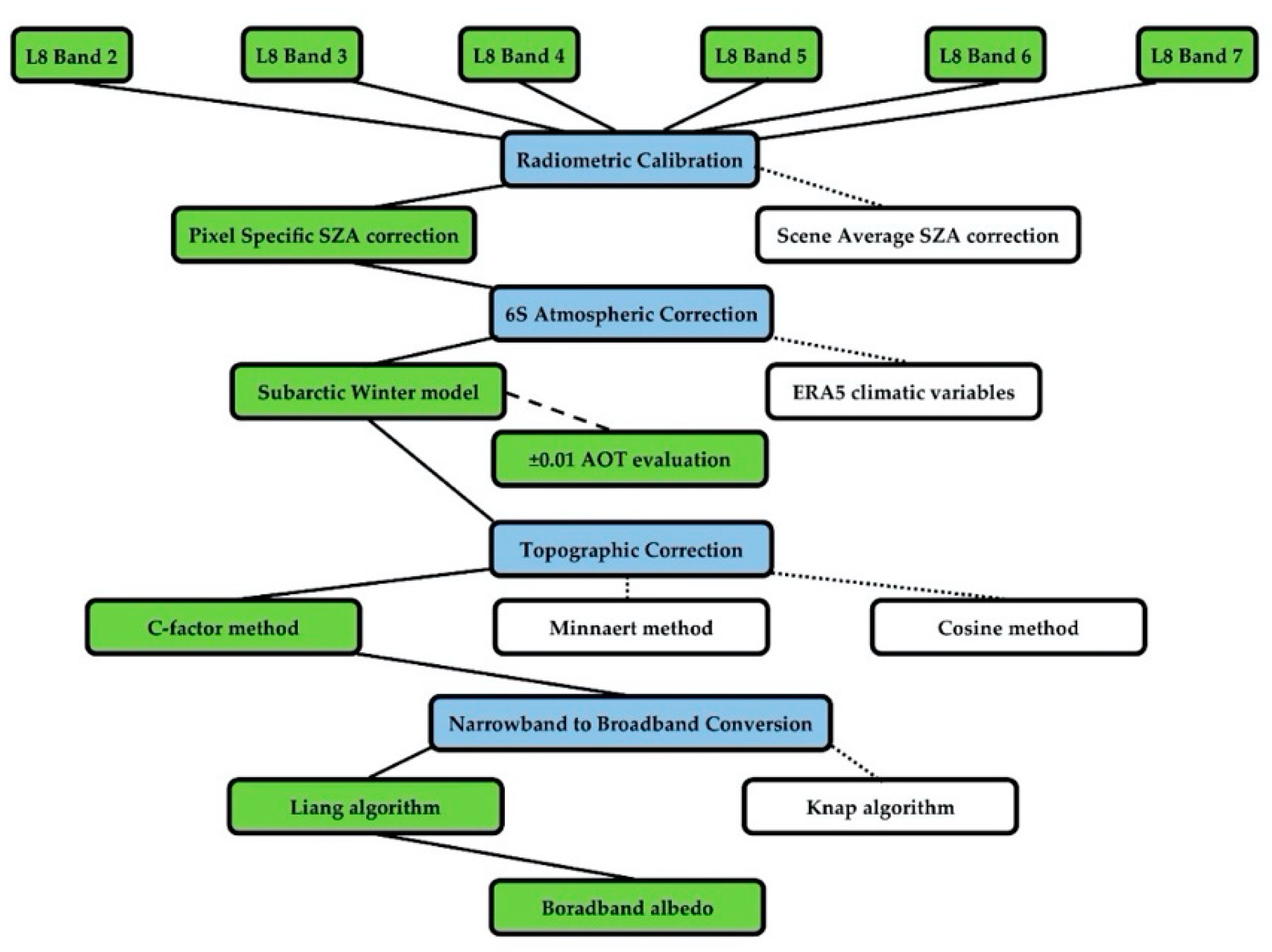
2.1. Satellite Data Processing

2.1.1. Radiometric Calibration and SZA Correction

In order to be stored and transmitted efficiently, radiance measured by the Landsat sensor is converted to a quantized digital number (DN, dimensionless) and needs to be scaled back to the original value. First, Landsat DNs in each band were converted to top of atmosphere (TOA) reflectance, following the Landsat 8 (L8) Data User Handbook [37] using the rescaling coefficients in the metadata as follows:

$${{\rho }_{\lambda }}^{\prime }=M_{\rho }{Q}_{cal}+A_{\rho }$$

(6)

where ${{\rho }_{\lambda }}^{\prime }$ is the TOA planetary reflectance in band λ (without SZA correction), $M_{\rho }$ is the band-specific multiplicative rescaling factor, $A_{\rho }$ the band-specific additive factor from the Metadata file and $Q_{cal}$ is the quantized and calibrated standard product pixel values (DN). Two possible corrections were then evaluated: one using an average SZA correction for each scene, and the other using the SZA band generated from the Angle file of Landsat 8 (scene average SZA). The zenith correction on TOA reflectance is calculated as:

$${\rho }_{\lambda }=\frac{{{\rho }_{\lambda }}^{\prime }}{\cos \left({\theta }_{SZA}\right)}=\frac{{{\rho }_{\lambda }}^{\prime }}{\sin \left({\theta }_{SEA}\right)}$$

(7)

where ${\rho }_{\lambda }$ is the TOA reflectance in band λ with correction for the SZA, ${\theta }_{SEA}$ is the local sun elevation angle in degrees and ${\theta }_{SZA}$ is the local SZA (${\theta }_{SZA}$ = 90° − ${\theta }_{SEA}$) provided either as the average value for the scene (obtained from the metadata) or in the solar zenith band for each single pixel. A pixel-specific correction could be relevant to calculate the albedo in polar regions since the SZA can vary across a Landsat scene (±2°) and the scene-average SZA might not be sufficient to provide an accurate model of albedo in the study area, especially when SZA is very high (>60°) [38].

2.1.2. Atmospheric Correction

For the retrieval of surface reflectance, we carried out a correction of reflectance for atmospheric interference using the 6S radiative transfer code [39]. This correction was performed using GRASS i.atcorr tool, which provides standard atmospheric profiles, but also accepts user defined values to characterize the atmospheric layer above a given area. The required inputs are: (i) the geometrical conditions, that is the satellite source (in our case Landsat 8 OLI); (ii) date, time and central coordinates (longitude and latitude); (iii) the atmospheric model; (iv) an aerosol model, where we selected the continental one; (v) visibility (km) or aerosol optical thickness (AOT) at 550 nm to estimate attenuation of direct solar irradiance by aerosols. As regards the atmospheric model, we tested two possible models: subarctic winter, which was chosen despite the fact that our scenes only cover the summer period because it best resembles the climatological conditions of the polar areas, and a scene specific model with user-defined values. The inputs for the user-defined model are altitude (m), pressure (hPa), temperature (°C), H₂O and O₃ density (g/m³), which were retrieved from the ERA5 [40] atmospheric reanalysis global climate dataset produced by the European Centre for Medium-Range Weather Forecasts (ECMWF). AOT is generally very low for the Antarctic continent, from observations in the AERONET Aerosol Robotic Network datasets (https://aeronet.gsfc.nasa.gov/cgi-bin/draw_map_display_aod_v3 (accessed date 19 February 2021)), based on 7 stations distributed across the continent, i.e., Marambio (64.240°S, 56.625°W), ARM WAIS (79.471°S, 112.083°W), Utsteinen (71.950°S, 23.333°E), Vechernaya Hill (67.660°S, 46.158°E), Progress (69.378°S, 76.389°E), South Pole Obs NOAA (90.000°S, 70.300°E) and ARM McMurdo (77.849°S, 166.730°E), that provide AOT between the summer seasons 2013–2020. Here, the AOT ranges from 0.01 to 0.03, showing an average of 0.02. This value was used for the entire continent, given the low variability of AOT across Antarctica (both coastal areas and inland) and the absence of other ground stations in the vicinity of the in situ stations and corresponding LANDSAT scenes. Regarding the Greenland Ice Sheet, AOT is more heterogeneous: in the inland, given the lack of available AOT values from aerosol observing networks, we used data from the Modern-Era Retrospective analysis for Research and Applications, Version 2 reanalysis product (MERRA-2, [41]). On the dates analyzed, the AOT from MERRA-2 is on average 0.02, and such value was therefore applied in the inland of Greenland. In the coastal zones, AOT shows a larger variability; thus, we selected AOT measurements from the closest stations from the AERONET network. To test the sensitivity of the albedo model to the chosen AOT values, we compared the albedo obtained with the selected values with two additional runs obtained by adding and subtracting 0.01 to the AOT (e.g., in Antarctica, we provide two comparisons with models retrieved using an AOT of 0.01 or 0.03). Finally, vi) the mean target elevation a.s.l. (km) was derived from the Reference Elevation Model of Antarctica (REMA) Digital Terrain Model (DEM) [42] for Antarctica, resampled to 30 m spatial resolution and the Greenland Ice Mapping Project (GIMP) DEM [43] for the Greenland icesheet, also resampled to 30 m. This correction provides a surface reflectance dataset lacking topographic correction.

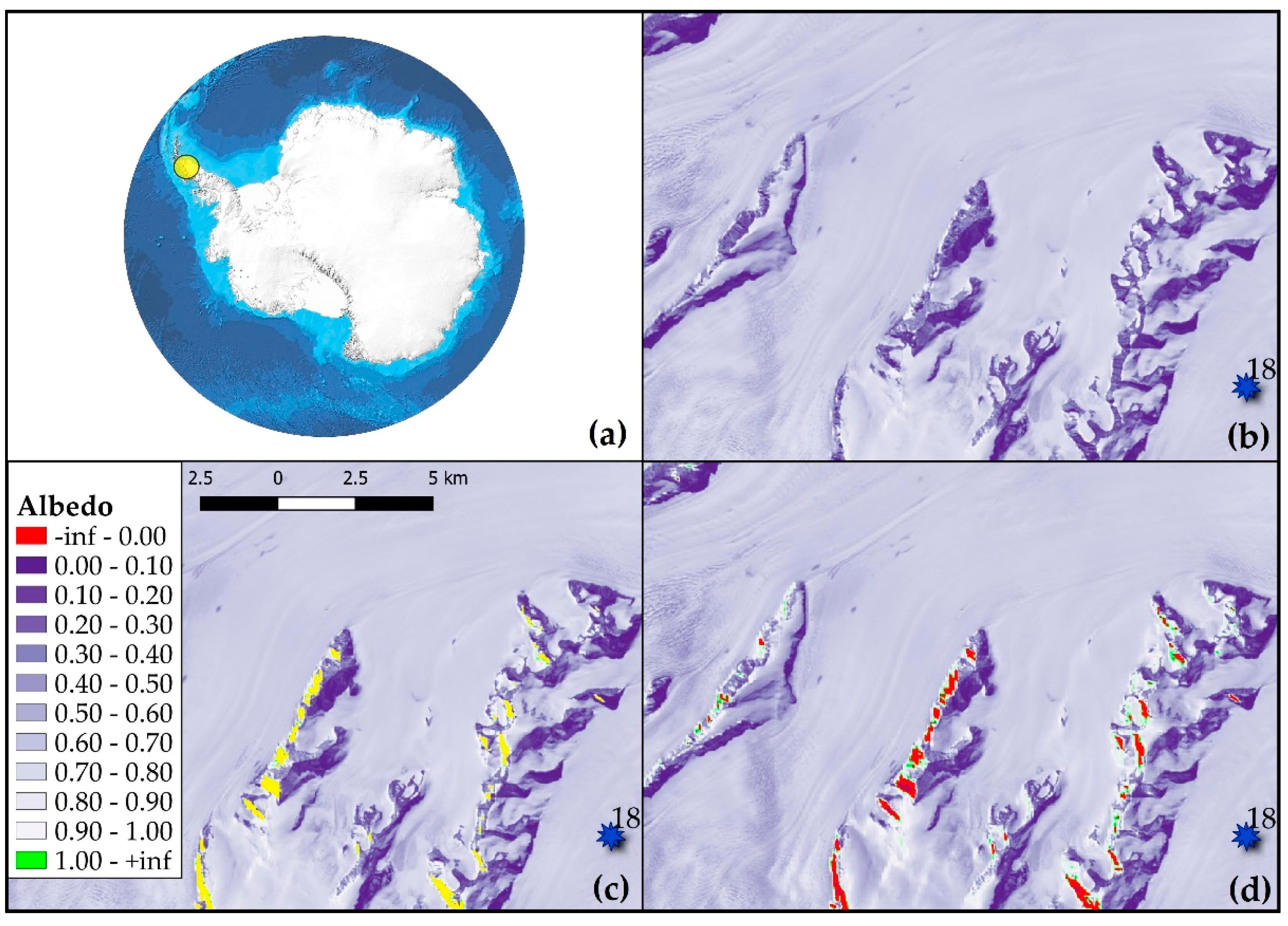
2.1.3. Topographic Correction

To compute the topographic correction of surface reflectance, different methods are available in GRASS GIS i.topo.corr tool, and we compared the following ones: c-factor, cosine and Minnaert. The first step is to produce an illumination model, which represents the cosine of the solar incident angle starting from the DEM. The formula is:

$$\cos i=\cos s\cos z+\sin s\sin z\cos \left(a-o\right)$$

(8)

where i is the incident angle, s is the terrain slope angle, z is the SZA, a is the solar azimuth angle and o is the terrain aspect angle.

Once the illumination model is calculated, it is possible to apply the topographic correction. The c-factor method is based on the following formula:

$$re{f}_c=re{f}_o\frac{\cos z+c}{\cos i+c}$$

(9)

where $re{f}_c$ is the corrected reflectance, $re{f}_o$ is the original reflectance and c is equal to a m⁻¹ from

$$re{f}_o=a+m\cos i$$

(10)

In summary, the tool needs a DEM and a value of SZA and solar azimuth angle, which are available from the Landsat metadata.

The cosine method is the simplest topographic correction, since it is represented by the following algorithm:

$$re{f}_c=\frac{re{f}_o\ast \cos z}{\cos i}$$

(11)

while the Minnaert method is described by:

$$re{f}_c=re{f}_o\ast {\left(\frac{\cos z}{\cos i}\right)}^k$$

(12)

where k is obtained by linear regression of

$$\ln \left(re{f}_o\right)=\ln \left(re{f}_c\right)-k\ast \ln \left(\frac{\cos i}{\cos z}\right)$$

(13)

2.1.4. Narrowband to Broadband Albedo Conversion

The final step concerns the estimation of broadband albedo (α), i.e., the albedo integrated over the entire solar spectrum. In our model, we used Liang albedo algorithm [34], which considers bands 2, 4, 5, 6 and 7 of the Landsat 8 OLI sensor, as suggested also by Naegeli et al. (2017) [32]. The algorithm is:

$$\alpha =0.356{\alpha }_2+0.130{\alpha }_4+0.373{\alpha }_5+0.085{\alpha }_6+0.072{\alpha }_7-0.0018$$

(14)

where α_x is the specific reflectance (equal to $re{f}_c$) of each band (and x the band number). The main advantage of this algorithm is that it considers contribution from a wider range of the spectrum than the others, allowing to capture the albedo changes due to changes in grain size, which have particularly large impact on near-infrared and shortwave infrared wavelengths [44]. We also evaluated the Knap algorithm [35], which is represented by the following equation:

$$\alpha =0.726{\alpha }_3-0.322{\alpha }_3^2-0.051{\alpha }_5+0.581{\alpha }_5^2$$

(15)

2.2. In Situ Broadband Albedo Data

With the intention of validating our satellite derived albedo after the correction process, we considered broadband albedo data from in situ stations located on the Antarctic and Greenland Ice Sheets (Figure 2). In detail, for the Antarctica we used broadband albedo from 7 AWSs owned by the Institute for Marine and Atmospheric Research Utrecht (IMAU) [18] in different zones of the Antarctic continent (Dronning Maud Land and Antarctic Peninsula) from 2013 to 2018 and 3 in situ stations from the World Radiation Monitoring Center—Baseline Surface Radiation Network (WRMC-BSRN, [17]), i.e., Concordia (DOM, [45]), Neumayer (GVN, [46]) and Syowa (SYO, [47]) Stations (respectively, located in Dome C, Dronning Maud Land and in proximity of Cosmonaut Sea). Regarding the 7 IMAU AWSs, they are equipped with Kipp and Zonen CNR1 or CNR4 radiometers, with a stated accuracy of ±10%. The sensor acquisition rate is 6 min, but the albedo values are then calculated as a 24 h moving average (in order to reduce errors due to sensor tilt and rime formation) [18]. The three BSRN stations are equipped with Kipp and Zonen pyranometers, respectively, CM22 for Concordia St., CMP22 for Neumayer St. and CMP21 for Syowa St. In each of the three BSRN stations, the pyranometer is situated at a height of 2 m and the sensor acquisition rate is 1 min, reporting separately the shortwave downwelling and upwelling radiation [45,46,47], from which we derived the albedo as a 24 h moving average for consistency with measurements from the IMAU network. On 9 out of 20 dates, the SZA at Neumayer and Syowa was higher than 60°, and the albedo appeared to increase compared to the dates with lower SZA (0.79 ± 0.027 at Neumayer and 0.76 ± 0.049 at Syowa when the SZA was < 60° compared to 0.88 ± 0.010 and 0.81 ± 0.035 when it was > 60°). This also led to much higher in situ albedo (up to 0.11) compared to satellite-derived albedo on these dates. We therefore assumed in situ albedo to be overestimated when the SZA was higher than 60°; in fact, this influence of high SZA on the albedo measured at in situ stations is well known and caused by an underestimation of the incoming radiation flux owing to the imperfect cosine response of the upward looking pyranometer [38]. To correct the values from these stations, we adopted the algorithm proposed by Briegleb et al. (1986) [48], derived by a scheme proposed by Dickinson (1983) [49], which normalizes albedo to a SZA of 60°. The algorithm was originally developed for vegetated surfaces and TOA reflectance, but was also used to estimate surface albedo by Pinker and Laszlo (1992) [50]. It is described as follows:

$${\alpha }_{60}={\alpha }_{SZA}\frac{1+2d\cos {\theta }_{SZA}}{1+d}$$

(16)

where α₆₀ is the normalized albedo considering SZA = 60°, ${\alpha }_{SZA}$ is the albedo measured at the in situ station at a specific SZA and d is equal to a constant, which varies between 0.1 and 0.4 depending on the type of surface and its dependence on SZA. [48,51,52]. We set d to 0.4 following Yang et al. (2008) [52], who suggests using this value for surface types with a high SZA dependence.

As regards the Greenland Ice Sheet, we used 4 AWSs of the Program for Monitoring of the Greenland Ice Sheet (PROMICE) [16], equipped with Kipp and Zonen CNR1 or CNR4 radiometers, acquiring data every 10 minutes (hourly averages transmitted). The stated accuracy is < 10% [53]. Again, even if some data are available since 2011, we analyzed albedo measurements acquired between 2014 and 2018. In

Table 1. Details of in situ stations considered in this study with the respective number of L8 scenes used for validation. * indicates dates excluded from the comparison (see Section 3.5). AWS stands for Automatic Weather Station, SZA for Solar zenith angle, DOM for Concordia Station, GVN for Neumayer Station, SYO for Syowa Station, EGP for EastGRIP Station, KAN B for Kangerlussuaq Station, QAS L for Quassimiut low Station and THU L for Thule low Station.

Dataset	In Situ Stations	Coordinates (Lat°; Long°)	Elevation (m a.s.l.)	Period	Landsat Scene	Landsat Dates	SZA (Deg)	Surface Type
IMAU
	AWS 05	−73.10; −13.17	360	1998–2014	178112	21/11/2013	62	Snow
						07/12/2013	61
	AWS 11	−71.17; −6.80	690	2007–2019	178110	07/12/2013 *	58	Snow
						24/01/2014 *	63
						27/01/2015 *	66
						28/02/2015 *	76
						15/02/2016 *	71
						12/10/2016 *	74
						16/01/2017 *	63
	AWS 14	−67.02; −61.50	50	2009–2015	217107	13/02/2015	68	Snow
	AWS 16	−71.95; 23.33	1300	2009–2015	156111	27/11/2013	64	Snow
						30/01/2014	69
						03/03/2014	79
						13/10/2014	76
						29/10/2014	70
						14/11/2014	66
						16/10/2015	74
						17/11/2015	65
						03/12/2015	63
	AWS 17	−65.93; −61.85	50	2011–2016	217106	11/10/2015	70	Snow
	AWS 18	−66.40; −63.73	70	2014–2018	217107	11/10/2015 *	71	Snow
						03/12/2017 *	58
						03/10/2018 *	74
	AWS 19	−70.95; 26.27	50	2014–2016	156110	16/10/2015	76	Snow
						17/11/2015	67
						03/12/2015	64
BSRN
	DOM	−75.10; 123.38	3233	2006–2020	089113	24/11/2014	61	Snow
						12/02/2015	70
						29/12/2015	60
						28/10/2016	68
						18/12/2017	59
						20/02/2018	73
						21/10/2019	71
	GVN	−70.65; −8.25	42	1992–2020	178110	07/12/2013	56	Snow
						29/12/2015	56
						15/02/2016	67
						02/03/2016	72
						12/10/2016	70
						16/01/2017	59
						05/12/2018	56
						09/01/2020	57
	SYO	−69.01; 39.59	18	1994–2019	148109	12/10/2014	69	Snow
						28/10/2014	63
						13/11/2014	59
						29/11/2014	56
						16/11/2015	58
						03/01/2016	55
						07/03/2016	73
						04/12/206	55
						22/02/2017	68
						20/10/2017	66
						08/01/2018	56
						23/10/2018	65
PROMICE
	EGP	75.62; −35.97	2660	2016–2019	007006	26/07/2016	57	Snow
						26/05/2017	55
						11/06/2017	53
						29/07/2017	57
						29/05/2018	54
	KAN B	67.13; −50.18	350	2011–2019	007013	29/04/2013 *	52	Rock
						31/05/2013	45
						19/08/2013	55
						06/08/2014	51
						23/05/2016	46
						08/06/2016	44
						10/07/2016	45
						26/07/2016	48
						10/05/2017	49
						27/06/2017	44
						29/07/2017	49
						14/08/2017	53
	QAS L	61.03; −46.85	280	2007–2019	002017	02/07/2014	39	Ice
						03/08/2014	45
						03/06/2015	40
						21/06/2016	39
						05/04/2017	56
						07/05/2017	45
						24/06/2017	39
						10/05/2018	44
						13/07/2018	41
						29/07/2018	44
						29/05/2019	41
	THU L	76.40; −68.27	570	2010–2019	032005	04/07/2014	54	Ice
						04/05/2015	61
						20/05/2015	57
						23/07/2015	57
						24/08/2015	66

further information about all the used in situ stations are reported and Figure 2 shows their locations. In general, all the satellite values of albedo used for the validation with the in situ data were averages of the 9 pixels surrounding the station, where the station is located in the center pixel. The only exception is represented by the Syowa Station, as it is in proximity of uncovered rock (distance lower than Landsat pixel resolution). For this station, we performed a comparison of a 9-pixel area NW of the station (approximately 60 m) to avoid rock disturbance. We also compared the average of the 4 surrounding pixels and the value of the specific pixel of the station. In both study areas, not all available in situ stations from the IMAU, WRMC-BSRN and PROMICE networks have been considered in this research, as for some of them we could not obtain a sufficient number of Landsat scenes for validation, owing to the absence of AOT values from nearby AERONET stations or excessive cloud cover in specific dates, also confirmed by the cloud cover value of the station datasets.

3. Results and Discussion

The results are displayed in five different subsections: the first concerns the validation of the albedo retrieval method in comparison with all in situ stations; then, each specific station dataset is considered, i.e., (i) IMAU AWSs [18] and (ii) BSRN stations [17] in Antarctica and (iii) PROMICE AWSs [16] in Greenland. Finally, we discuss possible reasons of discrepancy between satellite derived albedo and in situ observations.

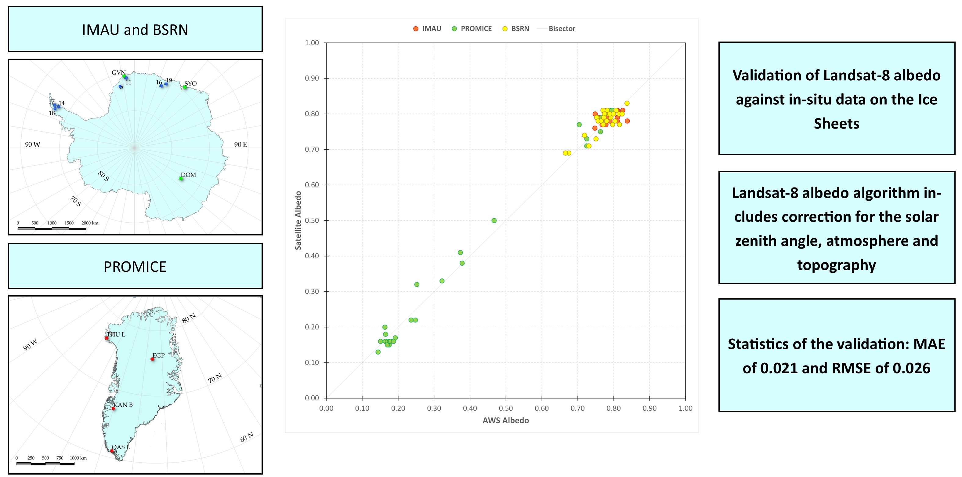
3.1. Method Validation

As described in Section 2, in order to validate the different combinations of input data or correction approaches for obtaining accurate albedo from satellite data, we compared different albedo values calculated following the same procedure, but varying the required inputs or parameters, as shown in the workflow of Figure 1. The specific statistics of the best combination and of each correction step are shown in

Table 2. Statistics of the albedo retrieval procedure, with the best combination in the first row and all other variants used for comparison (86 values). Statistics are: mean absolute error (MAE), standard deviation (STD), bias estimate (BE), correlation coefficient (Cc), root–mean–square error (RMSE) and bias-removed root–mean–square error (BRRMSE). Correlation is always significant at the 99% confidence level.

Dataset	MAE tot	MAE Antarctica	MAE Greenland	STD	BE	Cc	RMSE	BRRMSE
Proposed model	0.027	0.026	0.029	0.029	0.005	0.987	0.040	0.039
Ave. SZA c.	0.030	0.028	0.033	0.029	0.003	0.986	0.042	0.041
ERA5	0.028	0.028	0.028	0.030	0.011	0.987	0.041	0.040
AOT -0.01	0.028	0.027	0.030	0.029	0.007	0.987	0.040	0.040
AOT +0.01	0.028	0.026	0.031	0.028	0.002	0.987	0.040	0.040
Cosine c.	0.026	0.026	0.027	0.025	0.009	0.990	0.036	0.035
Minnaert c.	0.027	0.025	0.030	0.028	0.007	0.988	0.039	0.038
Knap a.	0.047	0.043	0.053	0.039	0.040	0.984	0.061	0.046
1 pixel	0.028	0.027	0.030	0.030	0.004	0.986	0.041	0.041
4 pixels	0.028	0.026	0.031	0.031	0.005	0.986	0.042	0.041

.

Examining the differences in albedo when changing inputs and parameters in the workflow, firstly, we calculated the albedo applying the pixel-specific SZA or scene average SZA corrections. The difference between the albedo calculated with the average and pixel specific SZA was very low, as the two datasets differed statistically (MAE) by 0.003, with only slightly worse values when using the average SZA, probably because of the low range of possible SZA within a Landsat image (±2°). The small statistical differences between the correction with scene-average and pixel specific SZA suggests that the pixel-specific SZA correction step is not crucial for albedo retrieval at high latitudes, although it did provide slightly better results.

As regards the atmospheric correction, we compared the albedo retrieved by using ERA5 climatic variables, against the one obtained when using the subarctic winter model in GRASS GIS. Again, the statistics were very similar, even if the atmospheric correction using the atmospheric model based on ERA5 variables showed slightly worse results. The standard deviation between in situ and satellite albedo processed by using ERA5 data was 0.030, the RMSE 0.041 and the BE increased to 0.011. (Best model: 0.029, 0.040 and 0.005, respectively). In addition, the statistics for the validation with Antarctic observations were worse since the MAE increased to 0.028, while the MAE for Greenland stations was slightly better (0.028). In this context, we demonstrated that the use of an available generic model for atmospheric correction, i.e., subarctic winter, provided the same, or even better, results than using detailed parameters, e.g., from ERA5 dataset. This might be caused by an incorrect representation of atmospheric layers at high latitudes in ERA5, given the scarcity of ground observations in the polar areas. Thus, the use of specific parameters in the 6S model might not be necessary at such high latitudes.

We also compared the results obtained by adding or subtracting 0.01 from the applied value of AOT. In fact, in the 6S model used for atmospheric correction, we simplified the AOT parameter by using a mean of 0.02 in Antarctica, considering that the parameter is constant throughout the average summer season, especially in the inland. According to Klok et al. (2003) [29], the uncertainty in AOT can propagate to the final albedo retrieval, leading to an error of 0.01. Thus, with the aim of minimizing the uncertainty, future research could better quantify AOT at the poles with specific campaigns. We did not find large differences among the three runs with different AOT, even if the default model provided always better statistics, especially compared to the albedo obtained when lowering the AOT by 0.01, apart from the BE. Nevertheless, looking at the two satellite albedo datasets obtained by varying the AOT by ±0.01, it is evident that an error of this magnitude in AOT should not cause a significant error in the calculated albedo. In addition, the strong correlation (0.985 99% confidence) between the proposed model and the one obtained when adding +0.01 to the AOT might suggest that AOT in Antarctica is well represented by an average range of 0.02–0.03.

As regards the topographic correction, in addition to the c-factor method, we also calculated the albedo by using two other methods: the cosine and the Minnaert methods. The cosine method showed good results, with statistics similar to the c-factor. Here, even if the model is more basic than c-factor (see Section 2.1.3) and the BE was higher by 0.004 and MAE by 0.001, the STD turned out to be slightly lower (0.025), as did the RMSE (0.036) and BRRMSE (0.035). Minimal statistical differences were also found between the c-factor and Minnaert method. However, looking at highly sloped areas (>15°) facing the same direction as the solar azimuth, e.g., mountain zones (Figure 3), the albedo from the cosine and Minnaert algorithms show some relevant problems.

In fact, compared to the c-factor method which provides albedo values for all kind of surfaces (Figure 3b), the Minnaert method cannot process area with high acclivity, which result in no data (yellow areas in Figure 3c). This is probably because Equation (12) uses a power function that can lead the values to overflow outside the possible ranges of floating-point numbers; in contrast, the cosine method overestimated or underestimated albedo in these zones (with values much higher than 1 or much lower than 0, green and red areas in Figure 3d, respectively).

In view of these differences, even if these sloped areas are quite uncommon across the ice sheets, we suggest using the c-factor method, since it provides at the same time results that are in agreement with in situ observations, while being able to obtain albedo values also for sloped surfaces, e.g., the ones represented in Figure 3.

Further still, we tested two separate algorithms to convert narrowband to broadband albedo: the Liang and Knap algorithms [34,35]. Broadband albedo calculated using the Knap algorithm (${\alpha }_{Knap}$) showed much worse statistics than the conversion using Liang algorithm (${\alpha }_{Liang}$). The MAE for ${\alpha }_{Knap}$ was 0.047, almost doubled compared to the MAE for ${\alpha }_{Liang}$ (0.027). Furthermore, for ${\alpha }_{Knap}$ the STD was 0.039, the RMSE increased to 0.061 and the BE to 0.040. In summary, the comparison between the two albedo datasets calculated using either Liang algorithm [34] or Knap algorithm [35], showed clear results in support of Liang algorithm. This is probably because Knap algorithm considers a lower number of bands than Liang algorithm (2 bands vs. 5), and might not be able to adequately represent albedo changes due to changes in grain size in the near-infrared and shortwave infrared wavelengths. Moreover, we checked whether there were any significant differences when considering 9, 4 or 1 pixels in the satellite image around the in situ station. Once more, the three datasets were very similar and the use of 9 pixels shows a minor improvement in results. The general statistics present only variations of a few thousandths. This might depend on the great homogeneity of the polar areas, characterized by wide, highly reflective surfaces.

In summary, our proposed model, i.e., the best combination of corrections reported in green in Figure 1 and in the first row in Table 2, showed a RMSE and a BRRMSE of 0.040 and 0.039 respectively, a BE of 0.005, an STD of 0.029, a correlation of 0.987 (p < 0.01) between in situ and satellite data and a MAE of 0.027. The MAE from the validation of satellite- albedo using in situ data was lower for the Antarctic Ice Sheet (IMAU and BSRN in situ stations, 53 scenes), than in the Greenland Ice sheet (PROMICE AWSs, 33 scenes), with a value of 0.026 against 0.029.

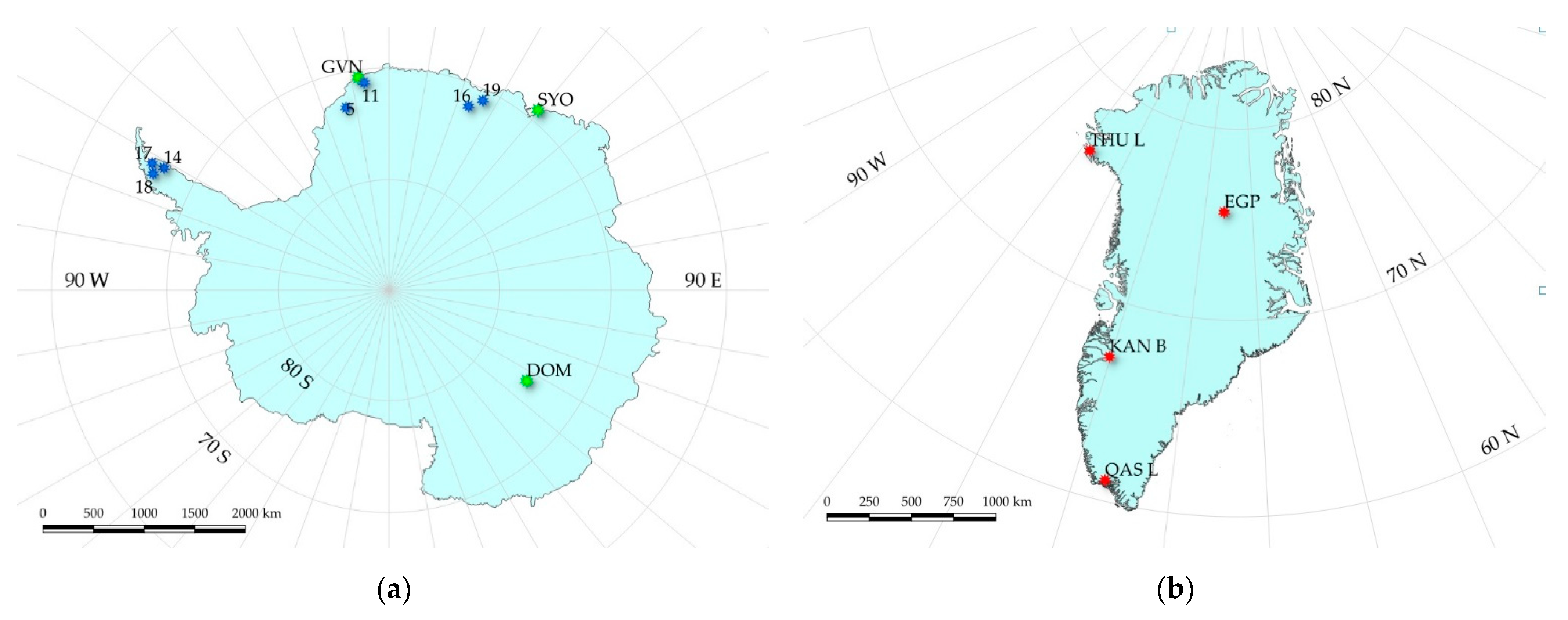
3.2. IMAU AWSs (Antarctica)

We considered seven IMAU AWSs in Antarctica [18], obtaining data consistent with Landsat 8 temporal range (2013–present). These AWSs provide broadband albedo, thus we compared the data with those calculated using Liang algorithm [34]. The total MAE between AWS observations and satellite derived albedo was 0.033 and STD was 0.026, based on 26 measurements. However, such an MAE might be due to the high MAE at AWS 11 (0.043 MAE) and 18 (0.077 MAE), which generally showed larger differences in comparison with the other stations. In fact, no other AWS reached a MAE of 0.040.

AWSs 5 and 11 are situated in western Dronning Maud Land, in proximity of the sea (Atlantic Ocean). 2 Landsat scenes were used for comparison with AWS 5, resulting in a MAE of 0.020 and 0.030 (thus a mean of 0.025); here, satellite albedo was generally slightly lower than AWS albedo. For AWS 11, we considered 7 Landsat scenes. The MAE of the difference between satellite and in situ albedo on these 7 dates was 0.043 and in every case the satellite derived albedo was lower than ground observations, and was on average 0.80, consistently with the typical Antarctic snow albedo [11,23]. AWS-based albedo had much higher values, even higher than 0.85 (which is typical of fresh snow). All dates of this station were affected by cloud cover, which was always >20%, which might explain the higher values compared to satellite-derived albedo, as the albedo is usually larger under clouds than in clear-sky conditions [55,56].

AWSs 14, 17 and 18 are situated in the northern part of Antarctic peninsula. AWS 14 and 17 had 1 coincident Landsat scene; at AWS14, Landsat derived and in situ albedo showed the same value, while the MAE was 0.030 at AWS 17. The albedo from 3 Landsat scenes was used for comparison with AWS 18, showing the highest absolute difference (0.077), as visible in Figure 4a.

In fact, while the observations from AWS18 showed a value typical of dry snow (>0.80), satellite derived albedo was always lower, showing values more typical of metamorphosized or wet snow (0.70–0.77, [57]). In particular, the MAE was 0.115, recorded on 11 October 2015. On that date, the satellite image showed lower albedo values in the proximity of the AWS, even typical of blue ice [58] while a value of 0.83 was measured at the AWS. The large difference at AWS 18 could be caused by the variations in surface conditions at the AWS, an inaccurate location recorded for this AWS due to ice flow, or residual sensor tilt that was not corrected by the 24 h moving average. This AWS is located at the base of an outlet glacier, where surface conditions could vary significantly over time: blue ice exposure can occur at the beginning of the summer season due to the effect of winter wind scouring, while in summer snow/ice melt can lead to the presence of superficial water. In addition, according to MEaSUREs ice flow velocity map (mostly derived from 2007–2016 data at 450 m spatial resolution [59]), the flow velocity of ice is 141 m/yr around the AWS, which might lead to a shift in the location of the station over time.

Finally, the last two AWSs (16 and 19) are situated in central-eastern Dronning Maud Land. AWS 16, used to validate the albedo from 9 Landsat scenes, showed a low MAE, 0.016. In addition, for 4 of these scenes, the error was even lower than 0.010. AWS 19 showed a MAE of 0.031 between AWS observations and satellite derived albedo, based on the validation of 3 Landsat scenes. Considering AWS16 and AWS19, we did not detect a bias between in situ and satellite data, since sometimes satellite-derived albedo underestimated in situ observations, sometimes overestimated them.

3.3. BSRN AWSs (Antarctica)

The best statistics were found for the validation of satellite albedo against BSRN in situ stations, based on a dataset of 27 Landsat scenes. In fact, the MAE for this dataset was 0.020 and the STD 0.012. 3 in situ stations were used for validation: DOM, GVN and SYO. The first one, DOM at Concordia Station, is the only one situated in the inner part of the continent and 7 dates were found to be suitable for the validation of satellite albedo, showing a MAE of 0.028, the highest of all three in situ stations. Here, 6 satellite-derived albedo values out of 7 were lower than field observations. In contrast, SYO showed no bias while at GVN satellite albedo was higher for most dates. At Neumayer and Syowa stations, the MAE was lower than 0.020: 0.019 and 0.015, respectively. 8 Landsat scenes were validated with data from GVN, and 12 with data from SYO (the most numerous dataset with KAN B AWS, see Section 3.4). As regards SYO in situ station, none of the data used for validation showed an absolute error greater than 0.030, while GVN station showed only one date with an absolute error > 0.030, on 16 January 2017.

3.4. PROMICE AWSs (Greenland)

As concerns the Greenland Ice Sheet, we compared Landsat derived albedo with data from four PROMICE AWSs [16], obtaining a dataset with 33 dates. In this case, the MAE between AWS measurements and satellite derived albedo was 0.029 and its standard deviation was 0.038. The only AWS situated in the inland is the EastGRIP Greenland site (EGP) AWS, at an average altitude of 2660 m a.s.l. Five dates were considered for EGP, resulting in a MAE of 0.020. Kangerlussuaq on land Station (KAN B), on the South-West of the Ice sheet, showed albedo values typical of rock (<0.20). A good agreement was found between albedo from this AWS and the one obtained from Landsat, except for the albedo from the first date used for validation (29 April 2013), that diverged from all the others, showing an absolute error of 0.222. Thus, the final MAE for the entire AWS is 0.035. Qassimiut low Station (QAS L), in the southernmost area of Greenland, showed a MAE of 0.024, based on 11 dates. The last considered station was the Thule low AWS (THU L), on the north-western tip of Greenland. As for EGP, since the station is located at high latitude (over 75° N), we could validate fewer Landsat 8 images (5). The MAE here was quite high, i.e., 0.034.

3.5. Analysis of the Cleaned Dataset

As discussed in the previous subsections, some of the scenes presented strong anomalies in the validation of satellite albedo using AWS observations from the IMAU dataset. In detail, AWSs 11 and 18 showed the largest differences. The former always shows high values typical of fresh snow (>0.85), which tend to be very unusual in Antarctica, and in fact, previous studies found lower albedo values for snow on the Antarctic plateau, around 0.80 or just slightly higher [3,11,27]. Moreover, high values of longwave-equivalent cloud cover (20–30%) were recorded at AWS 11 on several dates, even if the satellite imagery was cloud-free (according to the Landsat Metadata and visual check). Longwave equivalent cloud cover is not an observed value of cloudiness but is modelled from hourly values of downward longwave radiation and air temperature (at 2 m) [56,60]. According to Munneke et al. (2011) [61], this modeled cloud cover could differ from observed cloudiness (e.g., from satellite), leading to differences in modeled and observed net shortwave radiation at the surface and thus in albedo. In general, clouds have a relevant effect on albedo [62], especially when it is very high (e.g., for snowy surfaces, [44]). They alter the broadband albedo of a snow surface mainly by filtering out radiation at near-infrared (IR) wavelengths (>800 nm) more effectively than radiation in the visible region, thus changing the spectral composition of incoming radiation. The spectrally integrated albedo increases because the spectral albedo for visible wavelengths is higher than for near-IR wavelengths [56]. Cloudiness has been proposed as an explanation for higher variability in albedo measured at weather stations on the Antarctic shores [11], where most AWSs showing anomalous results are located. In addition to this cloud-cover issue, another station presented anomalous observations, with a MAE of 0.077, i.e., IMAU AWS 18 (see Section 3.2). In order to clean our dataset from the stations that showed anomalous data, we decided to exclude from the IMAU dataset AWS 11 (7 data) and 18 (3 data), providing a 43-scene dataset for Antarctica. Removing from the statistical calculations these 10 albedo values from AWS11 and AWS18, the MAE of Antarctic area dropped to 0.021. As concerns the Greenland Ice Sheet, one case of Landsat-derived albedo presented a large difference compared to field measurements, i.e., KAN B AWS on 29 April 2013, when the albedo observed at the station was much lower than the satellite derived one (0.55 against 0.77, a difference of 0.222). By examining the AWS dataset, we found high albedo variability in the week of satellite image acquisition, due to a snowfall event at the end of the boreal winter on the otherwise rocky surface where the station is located. In fact, albedo changed by more than 0.500 over a few days and since the PROMICE stations record hourly averages, such a difference can lead to an inaccurate validation of Landsat-derived albedo. Excluding the albedo from this date from the comparison, the MAE dropped to 0.023, based on a 32-scene dataset.

In general, excluding from the total statistics all these outliers, i.e., the data of 10 scenes in the Antarctic dataset and of 1 scene in the Greenland dataset, we obtained improved statistics for a 75-scene dataset (Figure 4b): a MAE of 0.021, STD of 0.015, RMSE of 0.026, BBRMSE of 0.025, a BE of −0.005 and a correlation coefficient of 0.995, with p < 0.01 (

Table 3. Statistics of the validation of satellite-albedo with in situ observations for the cleaned dataset, with the best option and all other variants used for comparison (75 values). Statistics are: mean absolute error (MAE), standard deviation (STD), bias (BE), correlation coefficient (Cc), root–mean–square error (RMSE) and bias-removed root–mean–square error (BRRMSE). Correlation is always significant at the 99% confidence level.

Dataset	MAE tot	MAE Antarctica	MAE Greenland	STD	BE	Cc	RMSE	BRRMSE
Proposed model	0.021	0.020	0.023	0.015	−0.005	0.995	0.026	0.025
Ave. SZA c.	0.024	0.022	0.027	0.017	−0.006	0.994	0.030	0.029
ERA5	0.021	0.021	0.022	0.016	0.001	0.995	0.026	0.026
AOT -0.01	0.022	0.020	0.024	0.015	−0.002	0.995	0.026	0.026
AOT +0.01	0.023	0.021	0.025	0.015	−0.007	0.995	0.027	0.027
Cosine c.	0.021	0.021	0.022	0.014	0.001	0.995	0.026	0.026
Minnaert c.	0.021	0.019	0.025	0.015	−0.002	0.995	0.026	0.026
Knap a.	0.040	0.035	0.047	0.029	0.032	0.992	0.049	0.037
1 pixel	0.022	0.021	0.024	0.017	−0.006	0.994	0.028	0.027
4 pixels	0.022	0.019	0.025	0.016	−0.004	0.995	0.027	0.027

).

Comparing these results with previous studies on polar ice sheets, Gusain et al. (2018) [63] found that MODIS albedo (from the MOD43B3 product) always overestimated AWS measurements in Antarctica, with a correlation coefficient of 0.86, a BE of 0.01 and a RMSE of 0.09; similar results were found by Stroeve et al. (2006) [64] in Greenland (RMSE > 0.06, BE < 0.02); Liang et al. (2005) [25] also reported a higher BE, slightly < 0.02 in Greenland. In other Earth regions (i.e., United States of America), Li et al. (2018) [65] found a lower BE and RMSE using higher spatial resolution satellite images (Sentinel-2A) compared to MODIS. Higher spatial resolution images are in fact less impacted by the spatial distribution of landscape features and structural changes across the surface (typical of coarser resolution images) and they are able to detect micro-scale differences as well.

Concerning possible reasons of discrepancies between our final satellite dataset and the in situ observations, surely relevant is the fact that data from in situ stations may represent local features that are averaged up in satellite-derived products with larger footprints, a problem that is likely to increase when coarser resolution data (e.g., MODIS, 500 m) are used in place of Landsat. In fact, our satellite data presented generally more constant values than the ones measured by the stations. Other sources of uncertainty for in situ albedo observations employed in this study include the intrinsic instrument measurement uncertainty, residual tilt errors, shifts in the station location over time and the correction of SZA dependence for albedo measured at GVN and SYO stations, using a formula that was originally developed for vegetated surfaces. However, this latter uncertainty only concerns 9 out of 86 measurements in our validation data set. While observations from ground stations are usually considered the most accurate and the standard method to assess the accuracy of satellite-derived products, our study shows that observations from AWSs might still be affected by large uncertainty, and that using manned stations (such as those from the BSRN network) might be more appropriate for validation. Besides, ground stations might show values that are not completely representative of their surroundings, and their use for validation of satellite data on the icesheets should be carefully evaluated.

As regards satellite-derived albedo, topographic correction and the related geolocation accuracy are considered to be the most important sources of errors, with an uncertainty up to 5% [29], depending on the incorrect co-registration of each DEM, even if in Antarctica such issue could be less relevant as large variations in altitude and slope are limited to very few areas. In addition, using Landsat 8 imagery, the DEMs proposed in this research represent the only available choices to maintain a similar spatial resolution between Landsat and DEM datasets. In fact, all other existing products in polar areas have a much coarser resolution (an order of magnitude larger), which would require down sampling to obtain a 30 m spatial resolution, likely introducing larger uncertainty.

A further correction not implemented in this study is anisotropic correction using BRDF models, which can be important in the retrieval of albedo from satellite data; its lack in our model could have negatively affected our satellite derived albedo and the observed differences might also be caused by its absence, according to Knap et al. (1999) [66]. While an anisotropic effect is certainly present on ice and snow surfaces in the polar regions, it has been omitted in this study because of the lack of a directly applicable correction model for Landsat data for such high values of albedo and SZA as are normally found on the ice sheets. In future research, approaches combining Landsat data with BRDF from MODIS, as done e.g., by He et al. (2018) [67], could be tested to evaluate whether including the anisotropic correction actually improves the agreement between satellite-derived albedo and in situ observations.

4. Conclusions

In this study, we employed the methodology proposed by Klok et al. (2003) [29] and also used by Fugazza et al. (2016) [19] to derive broadband albedo from Landsat 8 OLI satellite data at 30 m spatial resolution and validate it using observations from in situ stations located on the Antarctic and Greenland Ice Sheets. This model could allow future research to study local surface features by an optical point of view, considering that previous attempts provided only coarser resolution products (≥250 m) based on MODIS observations [6,23,24,25,26].

To validate satellite derived albedo, we performed a comparison between Landsat-retrieved albedo and different ground-based datasets, for a total of 86 scenes, while Fugazza et al. (2016) [19] only compared satellite albedo against data from one AWS and Wang et al. (2014) [27] performed a satellite inter-comparison between Landsat and MODIS albedo, following the method proposed by Klok et al. (2003) [29]. The difference from the latter research lies in a more detailed correction for the SZA, taking into account pixel-specific values, and in the narrowband to broadband albedo conversion. In fact, we found that Liang algorithm [34] provided better ground truth validation in the polar regions than Knap algorithm from the comparison with in situ observations [35]. The final proposed workflow (Figure 1) was obtained after we tested different variants of the model, by changing inputs and parameters at each stage of the albedo calculation, i.e., with average or pixel-specific SZA correction, atmospheric correction using a pre-defined model or with specific parameters from a reanalysis product, three different topographic correction approaches and two different algorithms for conversion of narrowband to broadband albedo. These comparisons allowed us to define the combination of corrections that could provide the best agreement with ground observations by in situ stations.

Three ground observation datasets were employed: (i) a dataset of seven AWSs from IMAU [18] located on the Antarctic Peninsula and Dronning Maud Land (Antarctica) and providing broadband albedo from 2014 to 2018, (ii) three stations from BSRN [17], located in three different areas of the continent, i.e., DOM (Dome C area), SYO (in the proximity of Cosmonaut sea) and GVN (Dronning Maud Land) from 2013 to present and iii) a dataset from PROMICE [16] of four AWSs located on the Greenland icesheet (both inland and coastal and southern and northern areas) from 2013 to 2019. In total, using data from 14 different in situ stations, we compared 86 albedo measurements on the Greenland and Antarctic icesheets, 33 in Greenland and 53 in Antarctica, obtaining a MAE between ground observations and satellite derived albedo of 0.027. In detail, the validation for stations on the Antarctic Ice Sheet showed a lower value compared to the Greenland Ice Sheet, with a MAE of 0.026 against 0.029. However, excluding 10 anomalous albedo values from the IMAU dataset and one from PROMICE, we compared a cleaned 75-scene dataset, which showed a lower MAE of 0.021 (0.020 for Antarctica and 0.023 for Greenland), a STD of 0.015, a RMSE of 0.026 and BRRMSE of 0.025, a BE of −0.005 and a correlation coefficient of 0.995 (p < 0.01).

Our study provides relevant findings for future polar sciences analysis at high resolution; to further extend and validate it, our model could be tested on previous satellites of the Landsat family, i.e., Landsat 5 ETM and Landsat 7 ETM+ as well as other satellite products at a similar spatial resolution, e.g., Sentinel 2 or ASTER.

References

1. Schaepman-Strub, G.; Schaepman, M.E.; Painter, T.H.; Dangel, S.; Martonchik, J.V. Reflectance Quantities in Optical Remote Sensing—Definitions and Case Studies. Remote Sens. Environ. 2006, 103, 27–42. [Google Scholar] [CrossRef]
2. Grenfell, T.C. Albedo. Encyclopedia of Snow, Ice and Glaciers; Singh, V., Singh, P., Haritahya, U., Eds.; Springer: Dordrecht, The Netherlands, 2011. [Google Scholar]
3. Grenfell, T.C.; Warren, S.G.; Mullen, P.C. Warren Reflection of Solar Radiation by the Antarctic Snow Surface at Ultraviolet, Visible, and near-Infrared Wavelengths. J. Geophys. Res. 1994, 99, 18669–18684. [Google Scholar] [CrossRef]
4. Gay, M.; Fily, M.; Genthon, C.; Frezzotti, M.; Oerter, H.; Winther, J.-G. Snow Grain-Size Measurements in Antarctica. J. Glaciol. 2002, 48, 527–535. [Google Scholar] [CrossRef] [Green Version]
5. Warren, S.G.; Brandt, R.E.; Grenfell, T.C. Visible and Near-Ultraviolet Absorption Spectrum of Ice from Transmission of Solar Radiation into Snow. Appl. Opt. 2006, 45, 5320–5334. [Google Scholar] [CrossRef] [PubMed] [Green Version]
6. Gallet, J.-C.; Domine, F.; Arnaud, L.; Picard, G.; Savarino, J. Vertical Profile of the Specific Surface Area and Density of the Snow at Dome C and on a Transect to Dumont D’Urville, Antarctica—Albedo Calculations and Comparison to Remote Sensing Products. Cryosphere 2011, 5, 631–649. [Google Scholar] [CrossRef] [Green Version]
7. Picard, G.; Libois, Q.; Arnaud, L.; Verin, G.; Dumont, M. Development and Calibration of an Automatic Spectral Albedometer to Estimate Near-Surface Snow SSA Time Series. Cryosphere 2016, 10, 1297–1316. [Google Scholar] [CrossRef] [Green Version]
8. Frezzotti, M.; Gandolfi, S.; Marca, F.L.; Urbini, S. Snow Dunes and Glazed Surfaces in Antarctica: New Field and Remote-Sensing Data. Ann. Glaciol. 2002, 34, 81–88. [Google Scholar] [CrossRef] [Green Version]
9. Scambos, T.A.; Frezzotti, M.; Haran, T.; Bohlander, J.; Lenaerts, J.T.M.; Van Den Broeke, M.R.; Jezek, K.; Long, D.; Urbini, S.; Farness, K.; et al. Extent of Low-Accumulation “wind Glaze” Areas on the East Antarctic Plateau: Implications for Continental Ice Mass Balance. J. Glaciol. 2012, 58, 633–647. [Google Scholar] [CrossRef] [Green Version]
10. Das, I.; Bell, R.E.; Scambos, T.A.; Wolovick, M.; Creyts, T.T.; Studinger, M.; Frearson, N.; Nicolas, J.P.; Lenaerts, J.T.M.; van den Broeke, M.R. Influence of Persistent Wind Scour on the Surface Mass Balance of Antarctica. Nat. Geosci. 2013, 6, 367–371. [Google Scholar] [CrossRef] [Green Version]
11. Pirazzini, R. Surface Albedo Measurements over Antarctic Sites in Summer. J. Geophys. Res. 2004, 109, D20118. [Google Scholar] [CrossRef]
12. Picard, G.; Domine, F.; Krinner, G.; Arnaud, L.; Lefebvre, E. Inhibition of the Positive Snow-Albedo Feedback by Precipitation in Interior Antarctica. Nat. Clim. Chang. 2012, 2, 795–798. [Google Scholar] [CrossRef]
13. Lenaerts, J.T.M.; Lhermitte, S.; Drews, R.; Ligtenberg, S.R.M.; Berger, S.; Helm, V.; Smeets, C.; Van Den Broeke, M.R.; Van De Berg, W.J.; Van Meijgaard, E. Meltwater Produced by Wind–Albedo Interaction Stored in an East Antarctic Ice Shelf. Nat. Clim. Chang. 2017, 7, 58–62. [Google Scholar] [CrossRef] [Green Version]
14. Rusin, N.P. Meteorological and Radiational Regime of Antarctica. Jerus. Isr. Program Sci. Transl. 1961. [Google Scholar]
15. Bintanja, R.; Van Den Broeke, M.R. The Surface Energy Balance of Antarctic Snow and Blue Ice. J. Appl. Meteorol. Climatol. 1995, 34, 902–926. [Google Scholar] [CrossRef]
16. van As, D.; Ahlstrøm, A.P.; Andersen, M.L.; Citterio, M.; Edelvang, K.; Gravesen, P.; Machguth, H.; Nick, F.M. Programme for Monitoring of the Greenland Ice Sheet (PROMICE): First Temperature and Ablation Records. Geol. Surv. Den. Greenl. Bull. 2011, 23, 73–76. [Google Scholar]
17. Driemel, A.; Augustine, J.; Behrens, K.; Colle, S.; Cox, C.; Cuevas-Agulló, E.; Denn, F.M.; Duprat, T.; Fukuda, M.; Grobe, H.; et al. Baseline Surface Radiation Network (BSRN): Structure and Data Description (1992–2017). Earth Syst. Sci. Data 2018, 10, 1491–1501. [Google Scholar] [CrossRef] [Green Version]
18. Jakobs, C.L.; Reijmer, C.H.; Smeets, C.J.P.P.; Trusel, L.D.; van de Berg, W.J.; van den Broeke, M.R.; van Wessem, J.M. A Benchmark Dataset of in Situ Antarctic Surface Melt Rates and Energy Balance. J. Glaciol. 2020, 66, 291–302. [Google Scholar] [CrossRef] [Green Version]
19. Fugazza, D.; Senese, A.; Azzoni, R.S.; Maugeri, M.; Diolaiuti, G.A. Spatial Distribution of Surface Albedo at the Forni Glacier (Stelvio National Park, Central Italian Alps). Cold Reg. Sci. Technol. 2016, 125, 128–137. [Google Scholar] [CrossRef]
20. Azzoni, R.S.; Senese, A.; Zerboni, A.; Maugeri, M.; Smiraglia, C.; Diolaiuti, G.A. Estimating Ice Albedo from Fine Debris Cover Quantified by a Semi-Automatic Method: The Case Study of Forni Glacier, Italian Alps. Cryosphere 2016, 10, 665–679. [Google Scholar] [CrossRef] [Green Version]
21. Brock, B.W.; Willis, I.C.; Sharp, M.J. Measurement and Parameterization of Albedo Variations at Haut Glacier d’Arolla, Switzerland. J. Glaciol. 2000, 46, 675–688. [Google Scholar] [CrossRef] [Green Version]
22. Senese, A.; Maugeri, M.; Ferrari, S.; Confortola, G.; Soncini, A.; Bocchiola, D.; Diolaiuti, G. Modelling Shortwave and Longwave Downward Radiation and Air Temperature Driving Ablation at the Forni Glacier (Stelvio National Park, Italy). Geogr. Fis. Dinam. Quat. 2016, 39, 89–100. [Google Scholar]
23. Stroeve, J.; Box, J.E.; Wang, Z.; Schaaf, C.; Barrett, A. Re-Evaluation of MODIS MCD43 Greenland Albedo Accuracy and Trends. Remote Sens. Environ. 2013, 138, 199–214. [Google Scholar] [CrossRef]
24. Box, J.E.; van As, D.; Steffen, K. Greenland, Canadian and Icelandic Land-Ice Albedo Grids (2000–2016). Geol. Surv. Den. Greenl. Bull. 2017, 4, 53–56. [Google Scholar] [CrossRef] [Green Version]
25. Liang, S. Mapping Daily Snow/Ice Shortwave Broadband Albedo from Moderate Resolution Imaging Spectroradiometer (MODIS): The Improved Direct Retrieval Algorithm and Validation with Greenland in Situ Measurement. J. Geophys. Res. 2005, 110, D10109. [Google Scholar] [CrossRef] [Green Version]
26. Hui, F.; Ci, T.; Cheng, X.; Scambos, T.A.; Liu, Y.; Zhang, Y.; Chi, Z.; Huang, H.; Wang, X.; Wang, F. Mapping Blue-Ice Areas in Antarctica Using ETM+ and MODIS Data. Ann. Glaciol. 2014, 55, 129–137. [Google Scholar] [CrossRef] [Green Version]
27. Traversa, G.; Fugazza, D.; Senese, A.; Diolaiuti, G.A. Preliminary Results on Antarctic Albedo from Remote Sensing Observations. Geogr. Fis. Din. Quat. 2019, 42, 245–254. [Google Scholar]
28. Reijmer, C.H.; Bintanja, R.; Greuell, W. Surface Albedo Measurements over Snow and Blue Ice in Thematic Mapper Bands 2 and 4 in Dronning Maud Land, Antarctica. J. Geophys. Res. Atmos. 2001, 106, 9661–9672. [Google Scholar] [CrossRef] [Green Version]
29. Klok, E.L.; Greuell, W.; Oerlemans, J. Temporal and Spatial Variation of the Surface Albedo of Morteratschgletscher, Switzerland, as Derived from 12 Landsat Images. J. Glaciol. 2003, 49, 491–502. [Google Scholar] [CrossRef] [Green Version]
30. Shuai, Y.; Masek, J.G.; Gao, F.; Schaaf, C.B. An Algorithm for the Retrieval of 30-m Snow-Free Albedo from Landsat Surface Reflectance and MODIS BRDF. Remote Sens. Environ. 2011, 115, 2204–2216. [Google Scholar] [CrossRef]
31. Wang, J.; Ye, B.; Cui, Y.; He, X.; Yang, G. Spatial and Temporal Variations of Albedo on Nine Glaciers in Western China from 2000 to 2011. Hydrol. Process. 2014, 28, 3454–3465. [Google Scholar] [CrossRef]
32. Naegeli, K.; Damm, A.; Huss, M.; Wulf, H.; Schaepman, M.; Hoelzle, M. Cross-Comparison of Albedo Products for Glacier Surfaces Derived from Airborne and Satellite (Sentinel-2 and Landsat 8) Optical Data. Remote Sens. 2017, 9, 110. [Google Scholar] [CrossRef] [Green Version]
33. Fugazza, D.; Senese, A.; Azzoni, R.S.; Maugeri, M.; Maragno, D.; Diolaiuti, G.A. New Evidence of Glacier Darkening in the Ortles-Cevedale Group from Landsat Observations. Glob. Planet. Chang. 2019, 178, 35–45. [Google Scholar] [CrossRef]
34. Liang, S. Narrowband to Broadband Conversions of Land Surface Albedo I: Algorithms. Remote Sens. Environ. 2001, 76, 213–238. [Google Scholar] [CrossRef]
35. Knap, W.H.; Reijmer, C.H.; Oerlemans, J. Narrowband to Broadband Conversion of Landsat TM Glacier Albedos. Int. J. Remote Sens. 1999, 20, 2091–2110. [Google Scholar] [CrossRef]
36. Foga, S.; Scaramuzza, P.L.; Guo, S.; Zhu, Z.; Dilley, R.D., Jr.; Beckmann, T.; Schmidt, G.L.; Dwyer, J.L.; Hughes, M.J.; Laue, B. Cloud Detection Algorithm Comparison and Validation for Operational Landsat Data Products. Remote Sens. Environ. 2017, 194, 379–390. [Google Scholar] [CrossRef] [Green Version]
37. Zanter, K. Landsat 8 (L8) Data Users Handbook. In Landsat Sci. Off. Website. Available online: https://www.usgs.gov/media/files/landsat-8-data-users-handbook (accessed on 19 February 2021).
38. Picard, G.; Libois, Q.; Arnaud, L.; Vérin, G.; Dumont, M. Estimation of Superficial Snow Specific Surface Area from Spectral Albedo Time-Series at Dome C, Antarctica. Cryosphere Discuss 2016, 1–39. [Google Scholar] [CrossRef]
39. Vermote, E.F.; Tanré, D.; Deuze, J.L.; Herman, M.; Morcette, J.-J. Second Simulation of the Satellite Signal in the Solar Spectrum, 6S: An Overview. IEEE Trans. Geosci. Remote Sens. 1997, 35, 675–686. [Google Scholar] [CrossRef] [Green Version]
40. Hersbach, H.; Bell, B.; Berrisford, P.; Hirahara, S.; Horányi, A.; Muñoz-Sabater, J.; Nicolas, J.; Peubey, C.; Radu, R.; Schepers, D.; et al. The ERA5 Global Reanalysis. Q. J. R. Meteorol. Soc. 2020, 146, 1999–2049. [Google Scholar] [CrossRef]
41. Gelaro, R.; McCarty, W.; Suárez, M.J.; Todling, R.; Molod, A.; Takacs, L.; Randles, C.A.; Darmenov, A.; Bosilovich, M.G.; Reichle, R. The Modern-Era Retrospective Analysis for Research and Applications, Version 2 (MERRA-2). J. Clim. 2017, 30, 5419–5454. [Google Scholar] [CrossRef] [PubMed]
42. Howat, I.M.; Porter, C.; Smith, B.E.; Noh, M.-J.; Morin, P. The Reference Elevation Model of Antarctica. Cryosphere 2019, 13, 665–674. [Google Scholar] [CrossRef] [Green Version]
43. Howat, I.M.; Negrete, A.; Smith, B.E. The Greenland Ice Mapping Project (GIMP) Land Classification and Surface Elevation Data Sets. Cryosphere 2014, 8, 1509–1518. [Google Scholar] [CrossRef] [Green Version]
44. Wiscombe, W.J.; Warren, S.G. A Model for the Spectral Albedo of Snow. I: Pure Snow. J. Atmos. Sci. 1980, 37, 2712–2733. [Google Scholar] [CrossRef] [Green Version]
45. Lupi, A. Basic and Other Measurements of Radiation at Concordia Station; Institute of Atmospheric Sciences and Climate of the Italian National Research Council: Bologna, Italy, 2020. [Google Scholar]
46. Schmithüsen, H. Basic and Other Measurements of Radiation at Neumayer Station; Alfred Wegener Institute, Helmholtz Centre for Polar and Marine Research: Bremerhaven, Germany, 2020. [Google Scholar]
47. Ogihara, H. Basic and Other Measurements of Radiation at Station Syowa; National Institute of Polar Research: Tokyo, Japan, 2019. [Google Scholar]
48. Briegleb, B.P.; Minnis, P.; Ramanathan, V.; Harrison, E. Comparison of Regional Clear-Sky Albedos Inferred from Satellite Observations and Model Computations. J. Clim. Appl. Meteorol. 1986, 25, 214–226. [Google Scholar] [CrossRef]
49. Dickinson, R.E. Land surface processes and climate—Surface albedos and energy balance. In Advances in Geophysics, Proceedings of the A Symposium Commemorating the Two-Hundredth Anniversary of the Academy of Sciences of Lisbon, Lisbon, Portugal, 12–14 October 1981; Academic Press: Cambridge, MI, USA, 1983; Volume 25, pp. 305–353. [Google Scholar]
50. Pinker, R.T.; Laszlo, I. Modeling Surface Solar Irradiance for Satellite Applications on a Global Scale. J. Appl. Meteorol. Climatol. 1992, 31, 194–211. [Google Scholar] [CrossRef] [Green Version]
51. Wang, Z.; Barlage, M.; Zeng, X.; Dickinson, R.E.; Schaaf, C.B. The Solar Zenith Angle Dependence of Desert Albedo. Geophys. Res. Lett. 2005, 32. [Google Scholar] [CrossRef]
52. Yang, F.; Mitchell, K.; Hou, Y.-T.; Dai, Y.; Zeng, X.; Wang, Z.; Liang, X.-Z. Dependence of Land Surface Albedo on Solar Zenith Angle: Observations and Model Parameterization. J. Appl. Meteor. Climatol. 2008, 47, 2963–2982. [Google Scholar] [CrossRef] [Green Version]
53. Citterio, M.; Van As, D.; Ahlstrøm, A.P.; Andersen, M.L.; Andersen, S.B.; Box, J.E.; Charalampidis, C.; Colgan, W.T.; Fausto, R.S.; Nielsen, S.; et al. Automatic Weather Stations for Basic and Applied Glaciological Research. GEUS Bull. 2015, 69–72. [Google Scholar] [CrossRef] [Green Version]
54. Arndt, J.E.; Schenke, H.W.; Jakobsson, M.; Nitsche, F.O.; Buys, G.; Goleby, B.; Rebesco, M.; Bohoyo, F.; Hong, J.; Black, J.; et al. The International Bathymetric Chart of the Southern Ocean (IBCSO) Version 1.0—A New Bathymetric Compilation Covering Circum-Antarctic Waters. Geophys. Res. Lett. 2013, 40, 3111–3117. [Google Scholar] [CrossRef] [Green Version]
55. Yamanouchi, T. Variations of Incident Solar Flux and Snow Albedo on the Solar Zenith Angle and Cloud Cover, at Mizuho Station, Antarctica. J. Meteorol. Soc. Jpn. Ser. II 1983, 61, 879–893. [Google Scholar] [CrossRef] [Green Version]
56. Munneke, P.K.; Reijmer, C.H.; Van den Broeke, M.R. Assessing the Retrieval of Cloud Properties from Radiation Measurements over Snow and Ice. Int. J. Climatol. 2011, 31, 756–769. [Google Scholar] [CrossRef] [Green Version]
57. Cuffey, K.M.; Paterson, W.S.B. The Physics of Glaciers; Academic Press: Amsterdam, The Netherlands, 2010. [Google Scholar]
58. Bintanja, R. On the Glaciological, Meteorological, and Climatological Significance of Antarctic Blue Ice Areas. Rev. Geophys. 1999, 37, 337–359. [Google Scholar] [CrossRef]
59. Rignot, E.; Mouginot, J.; Scheuchl, B. MEaSUREs InSAR-Based Antarctica Ice Velocity Map, Version 2; NASA DAAC at the National Snow and Ice Data Center: Boulder, CO, USA, 2017. [Google Scholar]
60. Jakobs, C.L.; Reijmer, C.H.; Kuipers Munneke, P.; König-Langlo, G.; Van Den Broeke, M.R. Quantifying the Snowmelt-Albedo Feedback at Neumayer Station, East Antarctica. Cryosphere 2019, 13, 1473–1485. [Google Scholar] [CrossRef] [Green Version]
61. Munneke, P.K.; van den Broeke, M.R.; Lenaerts, J.T.M.; Flanner, M.G.; Gardner, A.S.; van de Berg, W.J. A New Albedo Parameterization for Use in Climate Models over the Antarctic Ice Sheet. J. Geophys. Res. Atmos. 2011, 116. [Google Scholar] [CrossRef] [Green Version]
62. Oerlemans, J. The Microclimate of Valley Glaciers; Igitur, Utrecht Publishing & Archiving Services: Utrecht, The Netherlands, 2010. [Google Scholar]
63. Gusain, H.S.; Singh, D.K.; Mishra, V.D.; Arora, M.K. Estimation of Net Radiation Flux of Antarctic Ice Sheet in East Dronning Maud Land, Antarctica, During Clear Sky Days Using Remote Sensing and Meteorological Data. Remote Sens. Earth Syst. Sci. 2018, 1, 89–99. [Google Scholar] [CrossRef]
64. Stroeve, J.C.; Box, J.E.; Haran, T. Evaluation of the MODIS (MOD10A1) Daily Snow Albedo Product over the Greenland Ice Sheet. Remote Sens. Environ. 2006, 105, 155–171. [Google Scholar] [CrossRef]
65. Li, Z.; Erb, A.; Sun, Q.; Liu, Y.; Shuai, Y.; Wang, Z.; Boucher, P.; Schaaf, C. Preliminary Assessment of 20-m Surface Albedo Retrievals from Sentinel-2A Surface Reflectance and MODIS/VIIRS Surface Anisotropy Measures. Remote Sens. Environ. 2018, 217, 352–365. [Google Scholar] [CrossRef]
66. Knap, W.H.; Brock, B.W.; Oerlemans, J.; Willis, I.C. Comparison of Landsat TM-Derived and Ground-Based Albedos of Haut Glacier d’Arolla, Switzerland. Int. J. Remote Sens. 1999, 20, 3293–3310. [Google Scholar] [CrossRef]
67. He, T.; Liang, S.; Wang, D.; Cao, Y.; Gao, F.; Yu, Y.; Feng, M. Evaluating Land Surface Albedo Estimation from Landsat MSS, TM, ETM+, and OLI Data Based on the Unified Direct Estimation Approach. Remote Sens. Environ. 2018, 204, 181–196. [Google Scholar] [CrossRef]
Figure 1. Workflow of albedo calculation through the main 4 steps (blue boxes), with each corresponding tested variant (best ones in green boxes, others evaluated in white boxes); solid lines stand for best workflow, dotted lines for other tested variants and dashed line for the evaluation of different AOT values.
Remotesensing 13 00799 g001
Figure 2. Location of the in situ stations employed in this study, in Antarctica (IMAU–Institute for Marine and Atmospheric Research Utrecht in blue and BSRN–Baseline Surface Radiation Network in green) on the left (a) and in Greenland (PROMICE–Programme for Monitoring of the Greenland Ice Sheet in red) on the right (b).
Remotesensing 13 00799 g002
Figure 3. (a) International bathymetric chart of the Southern Ocean (IBCSO, [54]) showing the mountainous area in the Antarctic Peninsula (within the yellow circle) in proximity of IMAU AWS 18; (bd) broadband albedo raster maps of the yellow area, respectively calculated using: the c-factor method (b), Minnaert method (c) and the cosine method (d). No-data:represented in yellow.
Remotesensing 13 00799 g003
Figure 4. The plots show the validation of satellite retrieved albedo (Landsat 8 OLI) using in situ observations: (a) IMAU in red, BSRN in yellow (Antarctica) and PROMICE in green (Greenland), (b) cleaned dataset. The arrows indicate the anomalous data.
Remotesensing 13 00799 g004