Adjacent-Track InSAR Processing for Large-Scale Land Subsidence Monitoring in the Hebei Plain

Abstract

Large-scale land subsidence has threatened the safety of the Hebei Plain in China. For tens of thousands of square kilometers of the Hebei Plain, large-scale subsidence monitoring is still one of the most difficult problems to be solved. In this paper, we employed the small baseline subset (SBAS) and NSBAS technique to monitor the land subsidence in the Hebei Plain (45,000 km²). The 166 Sentinel-1A data of adjacent-track 40 and 142 collected from May 2017 to May 2019 were used to generate the average deformation velocity and deformation time-series. A novel data fusion flow for the generation of land subsidence velocity of adjacent-track is presented and tested, named as the fusion of time-series interferometric synthetic aperture radar (TS-InSAR) results of adjacent-track using synthetic aperture radar amplitude images (FTASA). A cross-comparison analysis between the two tracks results and two TS-InSAR results was carried out. In addition, the deformation results were validated by leveling measurements and benchmarks on bedrock results, reaching a precision 9 mm/year. Twenty-six typical subsidence bowls were identified in Handan, Xingtai, Shijiazhuang, Hengshui, Cangzhou, and Baoding. An average annual subsidence velocity over −79 mm/year was observed in Gaoyang County of Baoding City. Through the cause analysis of the typical subsidence bowls, the results showed that the shallow and deep groundwater funnels, three different land use types over the building construction, industrial area, and dense residential area, and faults had high spatial correlation related to land subsidence bowls.

1. Introduction

Groundwater depletion and related land subsidence is a severe problem in many countries around the world. Several major cities worldwide suffer from aquifer depletion and land subsidence [1] due to overexploitation of groundwater resources [2]. Land subsidence may be one of the most obvious environmental impacts of groundwater extraction [3]. Globally, the demand for fresh water is the main cause of this phenomenon because of the rapid population growth [4]. Industrial fresh water is usually supplied directly by pumping from aquifer systems, which leads to compaction of the compressible aquifer [5]. It is easy to cause damage to the surface and underground infrastructure and increase the risk of flood in coastal cities [5,6].

Hebei Plain has experienced serious land subsidence (see Figure 1) and is an area of serious groundwater depletion in China [7,8,9,10,11]. The amount of water resources in the Hebei Plain is less than 1% of China, while the cultivated area accounts for 5.28% [12]. Hebei Plain covers more than 80% of towns and more than 70% of the population of Hebei Province, and groundwater extraction accounts for 80%~85% of the total water resources [13]. Since 1970, the groundwater level has been falling under the influence of natural and man-made factors in the Hebei Plain [14]. Due to the overexploitation of groundwater and the high population density, it has caused large-scale land subsidence and other geological hazards [15]. In addition to groundwater, the mining of liquid mineral resources and increased surface loads have also aggravated land subsidence [11,16,17]. Interferometric synthetic aperture radar (InSAR), which appeared in the late 1980s [18], has been widely used to monitor ground deformation information [19,20], but it is extremely vulnerable to temporal and spatial decorrelation and atmospheric phase delay [21]. The TS-InSAR technology, represented by SBAS [22], permanent scatters InSAR (PS-InSAR) [23,24], can monitor the surface centimeter and even millimeter-level slow deformation for a long time. TS-InSAR has high accuracy, a wide monitoring range, and low cost compared with earlier geological disaster monitoring methods, which have their own advantages.

Multi-track data cannot be used directly to produce interferograms because of different datum and geometry. The research of 3-D and 2-D deformation monitoring using multi-source and multi-track synthetic aperture radar (SAR) data has become a hot spot [25,26,27,28], while there are relatively few studies the fusion of one-dimensional multi-track SAR data. In 2007, for the first time, Ketelaar et al. proposed a mathematical framework for the datum connection of multiple independent overlapping tracks, and discussed the SAR data fusion method of an adjacent-track under the radar coordinate system [29]. Since then, research studying the fusion of one-dimensional multi-track results has gradually begun [30,31,32,33,34,35,36,37,38]. Some methods aim to increase the spatiotemporal sampling rate or to connect time-series results having time-gapped through multi-track monitoring [32,33,34,35]. Others have only considered the offset between two track deformation rates to merge multi-track TS-InSAR results [36,37]. The time-series analysis of multi-track interferograms may cause the loss of the transient component of the deformation time-series [38].

Some studies have used TS-InSAR to monitor land subsidence in different cities in the Hebei Plain [39,40,41], but the first full coverage monitoring was completed by Zhang Yonghong et al. in 2016 [42]. This research addressed several challenges in full coverage and long-term (from 1992 to 2014) land subsidence monitoring, but only the offset between the two tracks is considered to merge the deformation rate maps. Recently, some studies have monitored the subsidence of the North China Plain [16,43,44]. However, this article focuses on the study of the fusion of adjacent-track TS-InSAR results and qualitatively analyzes the causes of subsidence from five aspects in the Hebei Plain. Therefore, based on the method proposed by Sergey Samsonov [45], this paper proposes a novel data fusion flow for the generation of land subsidence velocity of adjacent-track to merge the TS-InSAR results of two adjacent-tracks with overlapping regions. In addition, this method does not need to interpolate and correct the persistent scatterer (PS) point, which further reduces the error and improves the accuracy.

The main objectives of the paper are as follows:

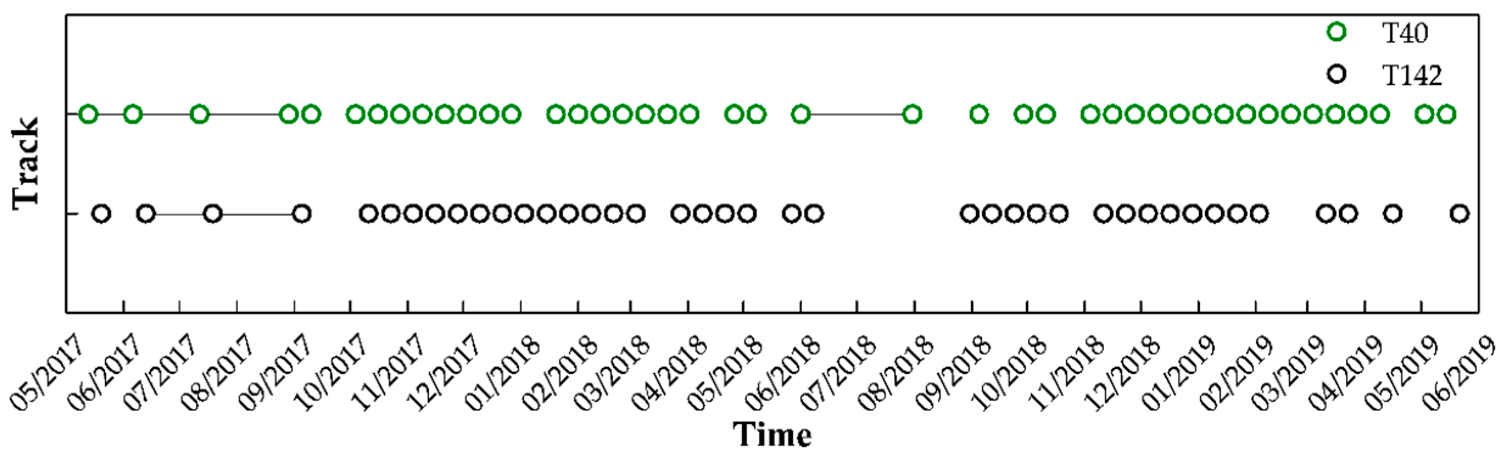
• Monitor land subsidence in the Hebei Plain (45,000 km²) by using two TS-InSAR techniques with 166 Sentinel-1A images of two adjacent-track from May 2017 to May 2019;
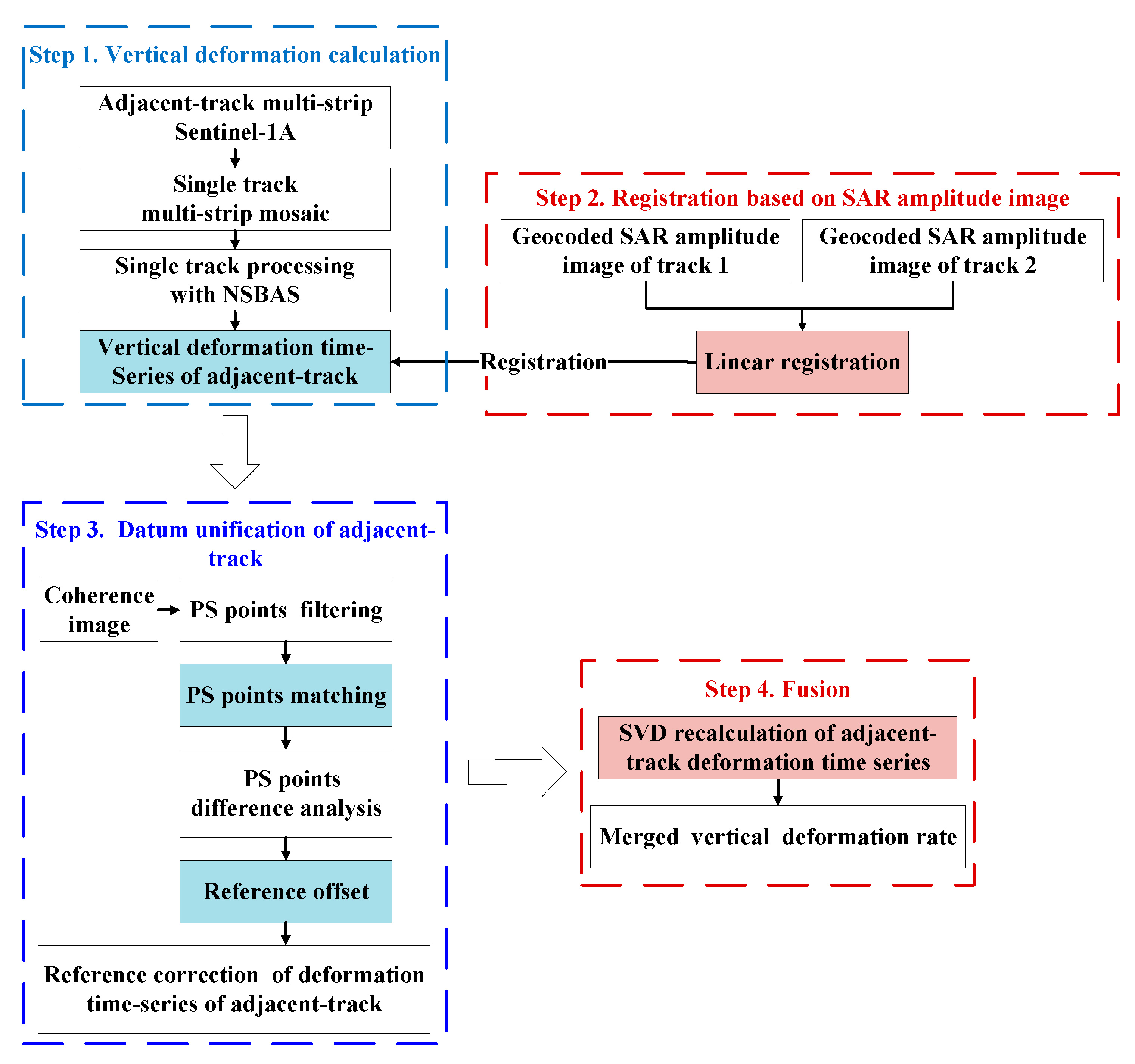
• Propose a novel data fusion flow for the generation of land subsidence vertical velocity of adjacent-track;
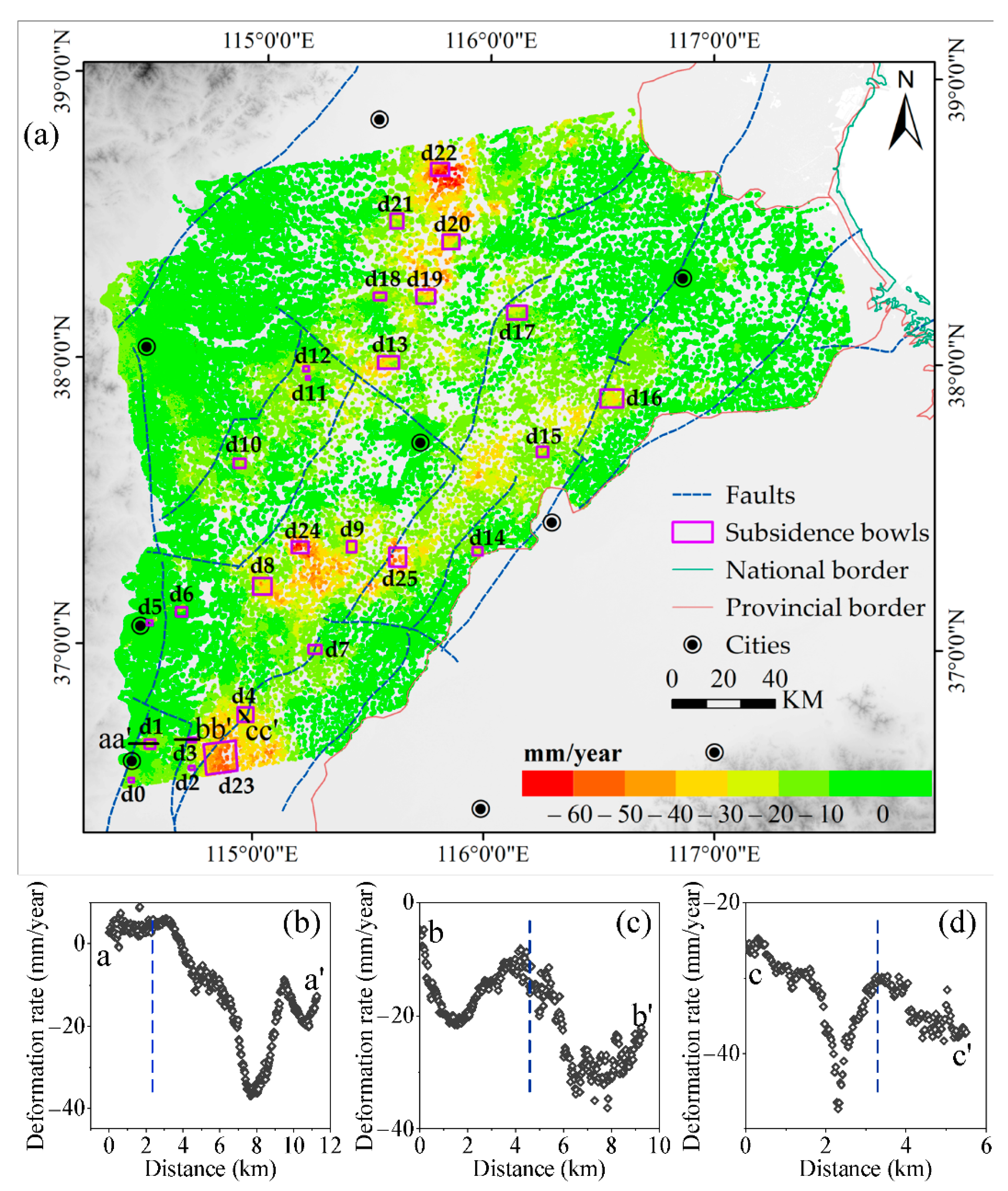
• Analyze the spatial and temporal evolution characteristics of subsidence features in the Hebei Plain and qualitatively analyze the causes of typical land subsidence bowls’ response to groundwater funnels, three land use types, and faults.

The rest of the paper is organized as follows: In Section 2, we introduce the study area and SAR data. In Section 3, TS-InSAR technologies are briefly introduced, and we propose a novel data fusion flow for the generation of the land subsidence vertical velocity of the adjacent-track. Then, data processing is briefly explained. In Section 4, several results and validations are presented. Finally, the discussion and conclusions of this study are summarized in Section 5 and Section 6, respectively.

2. Study Area and Data

2.1. Study Area

The Hebei Plain is located in the Hebei Province of China and forms the northern part of the North China Plain. The study area is outlined by a red border in Figure 2, covering most of the Hebei Plain and involving seven cities, namely Handan, Xingtai, Shijiazhuang, Hengshui, Cangzhou, Baoding, and Langfang. The study area is approximately 45,000 km² (114.280–117.610E, 36.492–38.911N). The Hebei Plain has a flat topography, and the terrain is high in the northwest and low in the southeast. The ground elevation changes from 100 m in front of the mountain to 2–3 m along the Bohai Sea. There are two river basins flowing through the Hebei Plain, namely the Haihe River and the Luanhe River. The Hebei Plain belongs to a continental monsoon climate. The annual average temperature is 10–25 °C. The average annual precipitation from 2018 to 2019 is about 475 mm in Hebei Province [46,47]. The annual precipitation is mainly concentrated in summer, and there is less in spring than in winter. The total amount of water resources were 4065 and 9119 million cubic meters in 2018 and 2019, respectively, which are less than the multi-year average water resources in Hebei Province [46,47]. The shallow groundwater level in the Hebei Plain dropped by an average of 0.13 and 0.58 m between 2018 and 2019, respectively [46,47]. The detailed information of groundwater level changes in 2018 and 2019 are shown in Figure 3 and

Table 1. Areas of shallow groundwater level change (adapted from [46,47]).

Year	Areas of Shallow Groundwater Levels Falling	Areas of Shallow Groundwater Levels Rising
2018	Southern Handan Central Hengshui Central Shijiazhuang Central and eastern Baoding	Central Handan Eastern Xingtai Western Shijiazhuang Western Baoding Southeastern Cangzhou
2019	Western Handan Central and southern Xingtai Most of Hengshui Southern and eastern Shijiazhuang Eastern and northern Baoding Most of Cangzhou Northwest Langfang	Western Shijiazhuang Western Baoding Southern Hengshui

. During 2018 and 2019, 55% of the water consumption in Heibei Province came from groundwater extraction [46,47].

2.2. Data

In total, 166 scenes of ascending Sentinel-1A [48] TOPS SAR images (C-band) along two adjacent-track four frames from May 2017 to May 2019 were used to monitor subsidence. As shown in

Table 2. Acquisition parameters of Sentinel-1A SAR data.

Track	Frame	Date Period	Date of Master Image	Number of SAR Data
40	117/122	13 May 2017–15 May 2019	11 October 2018	43 × 2
142	116/121	20 May 2017–22 May 2019	11 November 2018	40 × 2

and Figure 2, tracks 40 and 142 each had two frames. Track 40 (T40) included 86 scene images, and track 142 (T142) included 80 scene images. The dataset details are shown in Table 2 and

Table 3. Imaging parameters of Sentinel-1A SAR data.

Band	Polarization	Orbit Direction	Repeat Time (d)	Azimuth Resolution (m)	Slant Range Resolution (m)	Track
C	VV	Ascending	12	13.9	2.3	40/142

, and Figure 4. As can be seen from Figure 4, there were time-lags between the black lines, and the time was between 06/2017 and 09/2017 as well as 06/2018 and 09/2018. This is mainly due to the poor coherence of interferograms in summer. The one arc-second SRTM DEM (30*30 m) provided by the National Aeronautics and Space Administration (NASA) was used to remove topographic phases. Precise orbit determination (POD) [49] data were used for the orbital refinement and phase re-flattening.

3. Methodology

Section 3.1 provides a brief introduction to the basic theories of two TS-InSAR technologies, the SBAS and NSBAS [50,51,52] technologies. Section 3.2 introduces a novel data fusion flow for the generation of adjacent-track land subsidence velocity. Section 3.3 briefly introduces the data processing.

3.1. TS-InSAR Technologies

Here, we briefly describe the theories of the TS-InSAR techniques. A detailed description of the SBAS algorithm is provided by Berardino et al. [22]. First, the appropriate combination of differential interferograms are generated based on small temporal and spatial baseline threshold values. The least square method and singular value decomposition (SVD) method are used to calculate the line-of-sight (LOS) direction average deformation velocity and deformation time-series. For a given pixel l, there are $N_l$ interferograms and $M_l$ SAR images. There is a linear equation [22,50,51,52]:

$${\mathit{d}}_l={\mathit{G}}_l{\mathit{m}}_l$$

(1)

where ${\mathit{d}}_l$ is the phase vector of $N_l$ interferograms for pixel l; ${\mathit{m}}_l$ is a vector include $\left(M_{{}_l}-1\right)$ phase delay increments for pixel l; ${\mathit{G}}_l$ is a $N_l\times \left(M_{{}_l}-1\right)$ matrix composed of zeros and ones, constructed based on the phase of an interferogram; and ${\varphi }_{ij}^{\mathrm{l}}$ is the sum of the successive phase delays between SAR images i and j: ${\varphi }_{ij}^{\mathrm{l}}={\displaystyle \sum _{k=i}^{j-1}{m}_k^l}$ [50]. For a relatively large number of inversion pixels, ${\mathit{G}}_l^T{\mathit{G}}_l$ is singular. Use the SVD method instead of least square method to solve ${\mathit{d}}_l={\mathit{G}}_l{\mathit{m}}_l$.

We also followed NSBAS as described by Lopez-Quiroz et al. [50] to build the deformation time-series and deformation velocity maps. As time went by, the SBAS showed a clearly linear deformation, which caused a deviation in the time and thus a deviation in the deformation rate. In order to solve this problem, constraints were added to the TS-InSAR inversion instead of using the SVD method. The cumulative phase delay ${\varphi }_k^l$ for pixel l at time $t_k$ is defined by the following formula [50,51,52]:

$${\varphi }_k^l={\displaystyle \sum _{i=1}^{k-1}{m}_i^l}, 2\le k\le m_l$$

(2)

$${\varphi }_1^l=0$$

(3)

where $m_{\mathrm{k}}^l$ is the phase delay increment of the two successive SAR images at pixel l, and the following constraints are added in the inversion [50,51,52]:

$${\varphi }_k^l={\alpha }_t^l\left(t_k-t_1\right)+b_t^l{\left(t_k-t_1\right)}^2+e^l{B}_{\perp }^k+c_t^l$$

(4)

where $e^l{B}_{\perp }^k$ represents the DEM error phase related to the vertical baseline $B_{\perp }^k$ of each acquisition. We then solve, by least square inversion, the system ${\mathit{d}}^c={\mathit{G}}^c{\mathit{m}}^c$ [50]. The weight, γ, scales the additional matrix. If the SBAS network is complete, this method does not affect the inversion and is suitable for SAR data. If the SBAS network is incomplete and disconnected subsets appear, this method links these subsets [50].

$$\left[\begin{array}{c}{d}_1^l\\ ⋮\\ d_k^l\\ ⋮\\ d_{N_l}^l\\ 0\\ \\ ⋮\\ \\ 0\end{array}\right]=\left[\begin{array}{ccc}& \left[\begin{array}{ccccc}& & & & \\ & & & & \\ & & \hspace{1em} G_l\hspace{1em} & & \\ & & & & \\ & & & & \end{array}\right]& \left[\begin{array}{c}\begin{array}{c}\hspace{1em} 0\hspace{1em} \\ \end{array}\\ ⋮\\ \begin{array}{c}\\ \hspace{1em} 0\hspace{1em} \end{array}\end{array}\begin{array}{c}\hspace{1em} 0\hspace{1em} \\ \\ ⋮\\ \begin{array}{c}\\ \hspace{1em} 0\hspace{1em} \end{array}\end{array}\begin{array}{c}\begin{array}{c}\hspace{1em} 0\hspace{1em} \\ \end{array}\\ ⋮\\ \\ \hspace{1em}0\hspace{1em} \end{array}\begin{array}{c}\begin{array}{c} \hspace{1em}0\hspace{1em} \\ \end{array}\\ ⋮\\ \\ \hspace{1em}0\hspace{1em} \end{array}\right]\\ \gamma · & [\begin{array}{ccccc}0& \cdots & 0& \cdots & 0\\ 1& \ddots & & & ⋮\\ ⋮& \ddots & 0& & 0\\ ⋮& & \ddots & \ddots & ⋮\\ 1& \cdots & \cdots & 1& 0\end{array}& \begin{array}{cccc}0& 0& -B_{\perp }^1& -1\\ -(t_2-t_1)& -{(t_2-t_1)}^2& -B_{\perp }^2& -1\\ ⋮& ⋮& ⋮& ⋮\\ ⋮& ⋮& ⋮& ⋮\\ -(t_{M_l}-t_1)& -{(t_{M_l}-t_1)}^2& -B_{\perp }^{M_l}& -1\end{array}]\end{array}\right]\left[\begin{array}{c}{m}_1^l\\ \\ ⋮\\ \\ \\ m_{M_l}^l\\ a_t^l\\ b_t^l\\ e^l\\ c_t^l\end{array}\right]$$

(5)

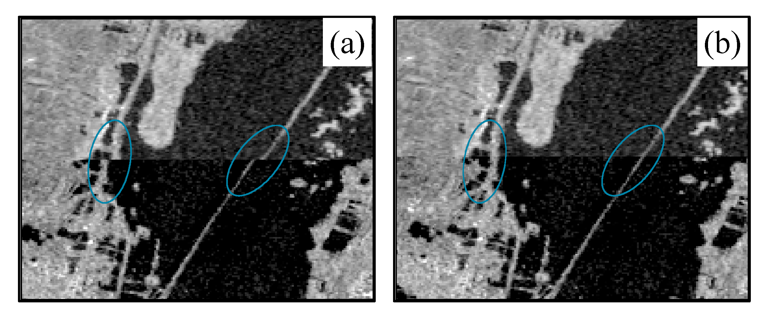
3.2. Fusion of TS-InSAR Results of Adjacent-Track Using SAR Amplitude Images (FTASA)

The single-track SAR data do not cover the Hebei Plain completely, which limits the large-scale subsidence monitoring, therefore, multi-track SAR data processing has come into being. However, there are at least three problems that need to be solved in the fusion of the adjacent-track TS-InSAR results. First, due to the different incidence angles of the adjacent-track, the imaging geometries are different. Second, the unwrapping reference points selected by TS-InSAR results from adjacent-track are inconsistent. Third, there is no connection between adjacent-track when we try to merge the adjacent-track results.

This paper proposes a fusion processing flow of adjacent-track TS-InSAR results based on SAR amplitude images (Figure 5). First, vertical deformation of every single track is retrieved. Second, adjacent-track deformation results are registered based on the SAR amplitude image. Third, the datum is unified by calculating the offset of the adjacent-track. Finally, adjacent-track deformation time-series fusion is solved by the SVD method. The detailed description of fusion processing flow is as follows:

Step 1: Vertical deformation calculation

InSAR is a side-view observation technique, and its direct observation result is LOS deformation. The LOS deformation observed by InSAR can be expressed as Equation (6):

$$d_{LOS}=\sin \vartheta \cos \phi \cdot d_e+\sin \vartheta \sin \phi \cdot d_n+\cos \vartheta \cdot d_u$$

(6)

where $d_e$, $d_n$, $d_u$ represent the east, north, and vertical deformations, respectively. $\vartheta$ is the incident angle, and $\phi$ is the angle between the satellite heading and north in a clockwise direction. Different tracks have different incidence angles. To eliminate this difference, we converted merely to vertical deformation by assuming the east and north land subsidence of Hebei is negligible [42,43,44]. Vertical deformation can be generated with Equation (7).

$$d_u=d_{LOS}/\cos \vartheta$$

(7)

Step 2: Registration of deformation results of adjacent-track based on SAR amplitude image

However, due to the different incident angles and other factors of the adjacent-track, the encoded deformation results of the adjacent-track are spatially deviated. Generally, remote sensing images are registered using the texture information of ground objects. However, the deformation results had no texture information, which makes it difficult to register. Therefore, we propose a registration method of adjacent-track deformation results based on SAR amplitude images. The affine transformation method is used for registration with Equations (8) and (9). This method first registers the encoded SAR amplitude images of adjacent-tracks within one pixel, and the registration transfer function is obtained to register deformation results of the adjacent-track. Pre-registration and post-registration comparison images of tracks 40 and 142 are shown in Figure 6.

$$X_{mas}={\displaystyle \sum _{i=0}^N{\displaystyle \sum _{j=0}^{N-i}{a}_{ij}{X}_{sla}^{{}^i}{Y}_{sla}^j}}$$

(8)

$$Y_{mas}={\displaystyle \sum _{i=0}^N{\displaystyle \sum _{j=0}^{N-i}{b}_{ij}{X}_{sla}^{{}^i}{Y}_{sla}^j}}$$

(9)

where $X_{mas}$ and $Y_{mas}$ are the coordinates of the master image; $X_{sla}$ and $Y_{sla}$ are the coordinates of the slave image; $a_{ij}$ and $b_{ij}$ are the polynomial coefficients to be solved, and N is the degree of the polynomial. Linear registration was used in this paper.

Step 3: Datum unification of adjacent-track

The reference points of the adjacent-track are usually difficult to keep consistent. In addition, the positions of the PS point of adjacent-track overlapping area are also not consistent. Here, we propose a unified reference method. First, filter the PS points using the overall coherence image for the single track. Second, extract the corresponding PS points of the adjacent-track based on geographic coordinates. Third, calculate the datum offset using Equation (10) [42] by analyzing the distribution of the homonymous point difference of the adjacent-track. The advantage of this method is that there is no need to interpolate the PS point of the adjacent-track. The offset is added to the adjacent-track to unify the datum.

$$\Delta t_{off}=\frac{1}{N}{\displaystyle \sum _{i=1}^N\left(t_{tra{2}_i}-t_{tra{1}_i}\right)}$$

(10)

Step 4: Fusion deformation time-series of adjacent-track

Suppose that $\left(d_{T_0^1}^1,d_{T_1^1}^1,\cdots ,d_{T_{N_1}^1}^1\right)$ and $\left(d_{T_0^2}^2,d_{T_1^2}^2,\cdots ,d_{T_{N_2}^2}^2\right)$ are the vertical deformation time-series of an arbitrary pixel in two tracks overlapping, respectively. Use the SVD method to obtain the merged time-series results with Equation (11), and the schematic diagram of the fusion is shown in Figure 7. Purple font $\left(T_0^1,T_1^1,\cdots ,T_{N_1}^1\right)$ are the times of track 1, and red font $\left(T_0^2,T_1^2,\cdots ,T_{N_2}^2\right)$ is the times of track 2, respectively.

$$AD=\Phi , A=\left(\begin{array}{c}{A}_0\\ A_1\\ ⋮\\ A_{N1+N2}\end{array}\right),D=\left(\begin{array}{c}{d}_0\\ ⋮\\ d_{N_1+N_2}\end{array}\right),\Phi =\left(\begin{array}{c}{d}_{T_1^1}^1-d_{T_0^1}^1\\ d_{T_1^2}^2-d_{T_0^2}^2\\ \begin{array}{c}⋮\\ d_{T_{N1}^1}^1-d_{T_{N1-1}^1}^1\end{array}\\ d_{T_{N2}^2}^2-d_{T_{N2-1}^2}^2\end{array}\right)$$

(11)

where $A_{\left(N_1+N_2\right)\left(N_1+N_2+1\right)}$ is the matrix composed of time intervals, and ${\mathbf{D}}_{N_1+N_2+1}$ is the unknown merged vertical deformation velocity time-series, and ${\Phi }_{N_1+N_2}$ is the adjacent-track vertical deformation time-series combinations.

3.3. Data Processing

The SBAS and NSBAS technique are applied to calculating the land deformation time-series using the four frames of tracks 40 and 142 of the 166 Sentinel-1A images by GAMMA and GIAnT [53,54]. Each SAR image is accurately registered to the master image. A total of 646 and 600 Sentinel-1A interferograms were generated for tracks 40 and 142, considering a maximum temporal and perpendicular baseline value of 360 days and 220 m, respectively. Concerning the interferogram coherence, 182 and 202 interferograms of tracks 40 and 142 were selected, respectively. Differential SAR interferograms were generated by using an SRTM DEM 1″. Furthermore, we also performed a 10 × 2 multilook operation for every S1A single interferogram with a 30 m × 30 m resolution. Each generated interferogram was first noise-filtered, and then unwrapped. The unwrapped phase signals were also calculated to the same reference pixel of each track. Subsequently, the LOS land deformation time-series were obtained from unwrapped DInSAR interferograms by using the SBAS and NSBAS technique. The atmospheric phase was filtered out from the obtained land deformation time-series. Moreover, assuming a simple linear relationship with topography, the stratified atmospheric phase contributions can be estimated from the data itself using a multi-scale approach [55]. We converted the LOS deformation time-series into the vertical time-series. We followed the process in Section 3.2 to get the merged subsidence velocity. First, the deformation time-series of tracks 40 and 142 were registered based on the SAR amplitude image. Second, the deformation time-series of tracks 40 and 142 eliminated the offset 0.9 mm. Finally, the deformation time-series of tracks 40 and 142 were merged using the SVD method.

4. Results

4.1. Fusion of Adjacent-Track PS Results

The vertical deformation velocity maps of tracks 40 and 142 are shown in Figure 8. The black line in Figure 8 is the overlapping area of tracks 40 and 142. It is clear to see that the NSBAS technique can generally provide more coherent pixels than SBAS techniques. Meanwhile, the NSBAS technique can provide entirely consistent results with SBAS techniques, despite some differences in the detailed characteristics. Therefore, we used the results of NSBAS for subsequent analysis. From Figure 8c,d, it can be clearly seen that the deformation trend of the overlapping area of tracks 40 and 142 were basically consistent. The subsidence velocity map of Hebei Plain was generated as shown in Figure 9.

From Figure 9, we can see that most regions of Hebei Plain were relatively stable. However, there exist about 26 apparent land subsidence bowls (labeled with letters from d0 to d25), and they tend to be connected in the administrative area. The maximum subsidence area was located in region d22 in Gaoyang County, where the deformation rate was up to −79 mm/year. As shown in Figure 10, six land subsidence bowls were found in Handan. Seven land subsidence bowls were found in Xingtai. Two land subsidence bowls were found in Shijiazhuang. Six land subsidence bowls were found in Hengshui. Three land subsidence bowls were found in Cangzhou, and two land subsidence bowls were found in Baoding. The detailed locations of 26 subsidence bowls are shown in

Table 4. Main information of the 26 subsidence bowls in six cities.

Cities	Subsidence Bowls	Locations	Average Subsidence Velocities (mm/year)	Maximum Subsidence Velocities (mm/year)
Handan	d0	Huaguanying Town of Hanshan District	−23	−44
	d1	Huangliangmeng Town of Congtai District	−17	−39
	d2	Xinan Town of Feixiang District	−15	−36
	d3	Guangfu Town of Yongnian District	−24	−39
	d4	Quzhou County of Quzhou District	−31	−48
	d23	Feixiang Town	−44	−65
Xingtai	d5	Daliangzhuang Town of Xiangdu District	0	−58
	d6	Rencheng Town of Renze District	−4	−27
	d7	Mingzhou Town of Wei County	−18	−56
	d8	Julu Town	−28	−59
	d9	Fenggang Street of Nangong City	−26	−43
	d10	Fenghuang Town of Ningjin County	−14	−38
	d24	Julu County	−55	−71
Shijiazhuang	d11	Xinji Town of Xinji City	−13	−35
	d12	Xinleitou Town of Xinji City	−24	−50
Hengshui	d13	Shenzhou Town of Shenzhou City	−28	−51
	d14	Zhengkou Town of Gucheng County	−18	−54
	d15	Jingzhou Town of Jing County	−21	−57
	d18	Anping County	−17	−32
	d19	Raoyang County	−29	−55
	d25	Zaoqiang County	−42	−62
Cangzhou	d16	Dongguang Town of Dongguang County	−26	−45
	d17	Xian County	−21	−39
	d20	Suning County	−30	−54
Baoding	d21	Liwu Town of Li County	−21	−50
	d22	Gaoyang Town and Yuejiazuo Town of Gaoyang County	−51	−79

.

4.2. Validation of the InSAR Results

In order to evaluate the accuracy of FTASA, we undertook a comparative analysis between the merged result acquired by only considering the offset (FO) and the merged result acquired by FTASA. Two merged results were also compared with the leveling results. The overlap area of tracks 40 and 142 had only two benchmarks. As shown in Figure 11, the average differences between the leveling results and FTASA, FO at the two benchmarks were 2 mm/year and 10 mm/year, respectively. This shows that FTASA has a higher accuracy than FO. We also plotted the difference between the two results as a histogram (see Figure 12). Difference of corresponding PS points of vertical deformation velocities in FTASA and FU were basically within [−10, 10] mm/year.

To quantitatively verify the accuracy of land subsidence monitoring using Sentinel-1A data by NSBAS, not only was a comparative analysis of the differences between the NSBAS, leveling results, and benchmark on the bedrock results performed, but the tracks 40 and 142 deformation results of overlapping were also comprehensively analyzed. Given the limited leveling data and benchmark on the bedrock data, the positions of the benchmark and the InSAR results were difficult to coincide. We extracted the nearest PS point corresponding to the benchmark. The leveling results were acquired from May 2017 to May 2019 and the two benchmarks on the bedrock results were acquired from December 2017 to June 2018. From Figure 13, we can see that the subsidence velocities obtained by InSAR were generally consistent with the leveling results and benchmark on the bedrock results. The overall RMSE between the leveling results and the InSAR results was 9 mm/year. The maximum and minimum errors were 17.5 mm/year and 1 mm/year, respectively. Overall, the InSAR results were highly correlated with the leveling results.

The deformation results of tracks 40 and 142 within the overlapped region were utilized. The histogram of the vertical deformation velocity difference within the overlapped region between tracks 40 and 142 is shown in Figure 14a. Statistical analysis showed that the 96% vertical deformation velocity difference of overlapping regions was within [−13, 13] mm/year, basically conforming to the normal distribution. The standard deviation was 7.37 mm/year. Figure 14b shows the linear fitting result of the vertical deformation velocity between tracks 40 and 142. The overlapping area of tracks 40 and 142 was approximately 14,000 km², with a total of 3,400,000 PS points. The linear fitting formula of tracks 40 and 142 was T40 = 0.96 × T142 + 0.60. The correlation coefficient was 0.89. We also selected four points (see Figure 9) in the overlapping area of tracks 40 and 142, and their deformation time-series are shown in Figure 15. It is clear that the time-series of tracks 40 and 142 were highly consistent. All these prove that the vertical deformation velocity of the two tracks had a good correlation.

5. Discussion

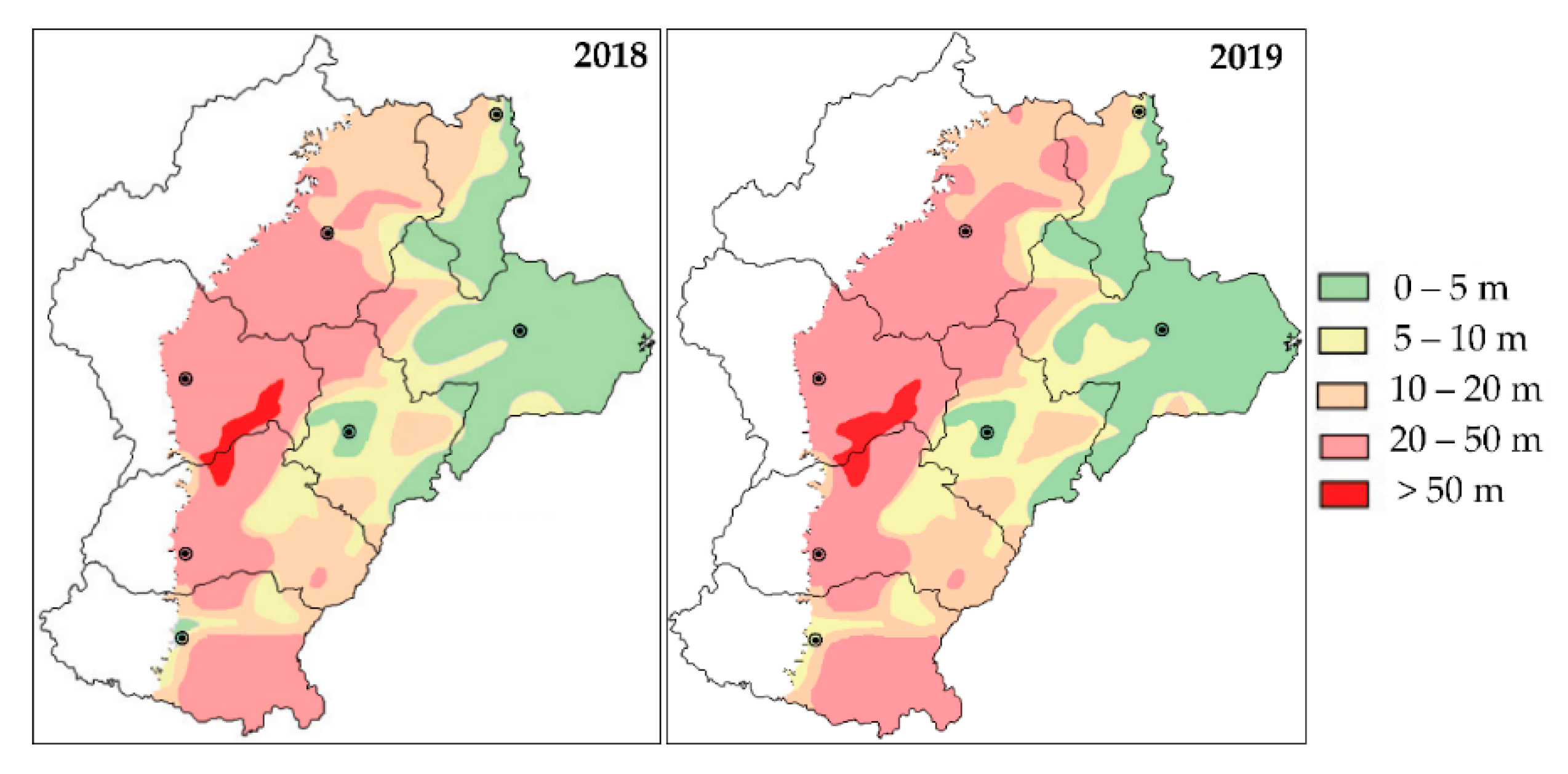
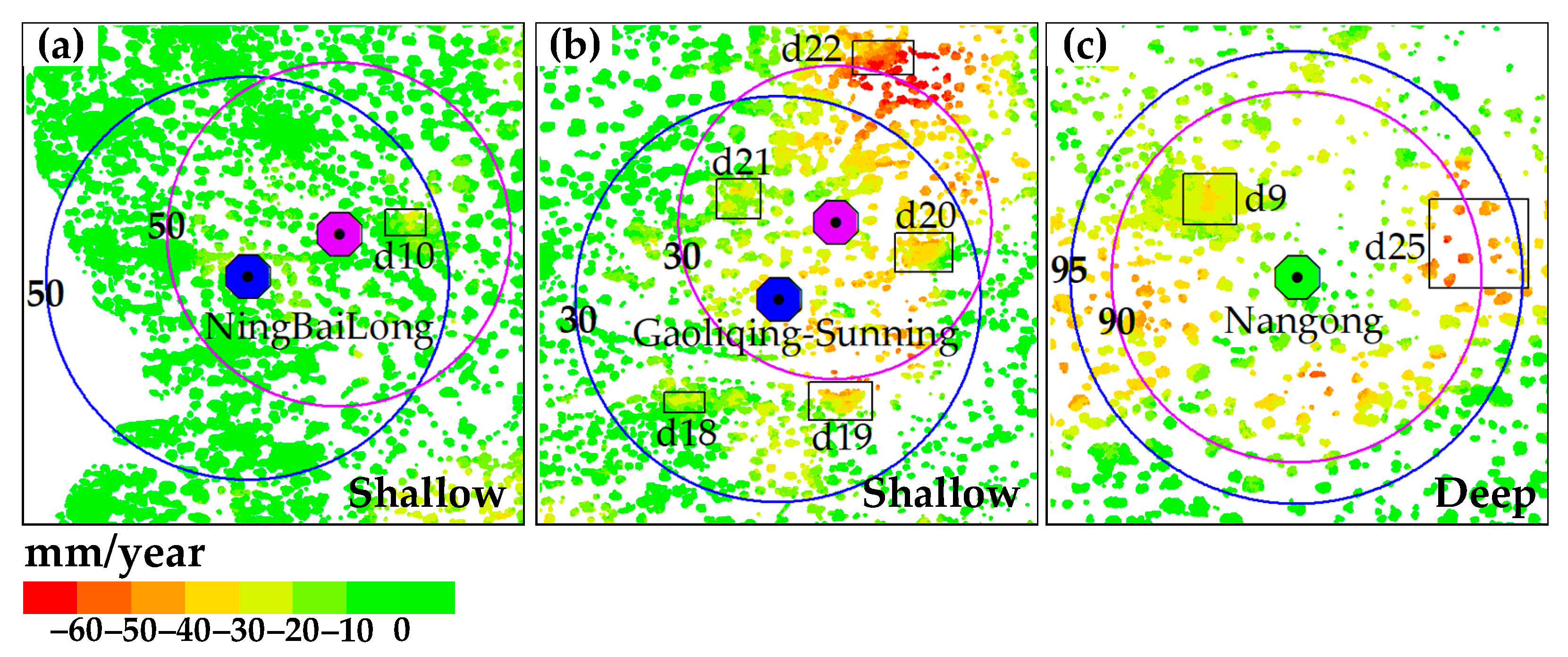
5.1. Groundwater Funnels and Land Subsidence

Shallow groundwater funnels like the Ningbolong funnel and Gaoliqing-Suning funnel, and deep groundwater funnels such as the Jizaoheng funnel and Nangong funnel are relatively large groundwater funnels in the Hebei Plain. The details of the groundwater funnels are shown in

Table 5. Groundwater funnels in Hebei Plain from 2018 to 2019.

Groundwater Funnels	Groundwater Level	Groundwater Funnels Centers		Depth Surrounding Funnel/m		Area/km2
		2018	2019	2018	2019	2018	2019
NingBaiLong	Shallow	Lijiaying, Ningjin County	Beitian, Baixiang County	50	50	1330	1566
Gaoliqing-Sunning	Shallow	Nanbaoxu, Lixian County	Hongshanbao, Lixian County	30	30	1160	2029
JiZaoHeng	Deep	Bali Village, Jingxian County	Bali Village, Jingxian County	90	95	508	842
Nangong	Deep	Jiaowang, Nangong City		90	95	664	947

. All the groundwater data were obtained from the Department of Water Resources of Hebei Province [46,47]. Figure 16 shows that the land subsidence bowls have a strong connection with the shallow or deep groundwater funnels. The subsidence bowl d10 (see Figure 16a) is located in the Ningbolong funnel within the scope of the funnels in 2018 and 2019. The Ningbolong funnel center is located in Lijiayingin in Ningjin County in 2018 and Beitian in Baixiang County in 2019. The buried depth of the funnel centers was 81.20 m in 2018 and 81.39 m in 2019. The area of the Ningbolong funnel area surrounded by the 50 m groundwater contour was 1330 and 1566 km² in 2018 and 2019, respectively. It can be seen from Figure 16b that the subsidence bowls d18–d21 are located in the Gaoliqing-Suning funnel, which is formed by the connection of the original Gaoliqing funnel and Suning funnel. Additionally, the centers of the Gaoliqing-Suning funnel are located in Nanbaoxu in Lixian County in 2018 and Hongshanbao in Lixian County in 2019. The buried depths of the Gaoliqing-Suning funnel centers were 37.70 m in 2018 and 40.70 m in 2019. The areas of the funnel area enclosed by the 30 m groundwater depth contour were 1160 and 2029 km² in 2018 and 2019, respectively. As can be seen in Figure 16c, subsidence bowls d9 and d25 were within the Nangong funnel, and the center of the Nangong funnel was located in Jiaowang in Nangong City. In 2018, the funnel center was buried at a depth of 99.20 m, and the groundwater depth contour was 90 m surrounded the funnel area with a 664 km² area. The burial depth of the funnel center was 108.70 m in 2019, and the 95 m groundwater depth contour enclosing the funnel area was 947 km². All in all, we found that there were six ground subsidence bowls in the shallow groundwater funnel, and two ground subsidence bowls in the deep groundwater funnel. There was a positive correlation between eight ground subsidence bowls and three groundwater funnels.

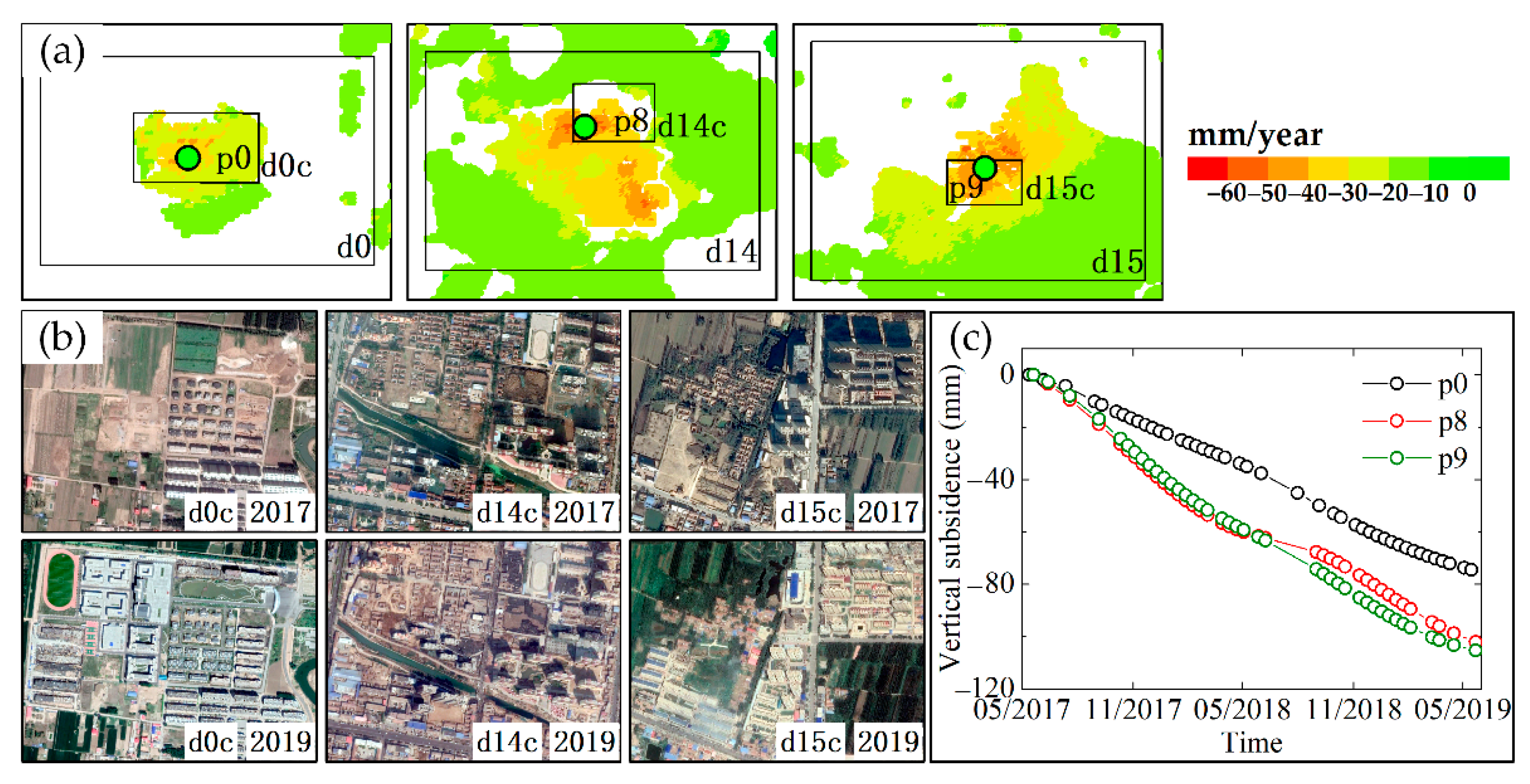
5.2. Building Constructions and Land Subsidence

Figure 17a shows the vertical deformation velocity map in three bowls (d0, d14, and d15) from May 2017 to May 2019. Three remarkable subsidence bowl centers (d0c, d14c, and d15c) associated with building construction were successfully detected. Two groups of Google Earth images over three subsidence bowl centers (Figure 17b) acquired in 2017 and 2019, respectively, show the detailed changes in the building construction process. Either large-scale buildings were built in these three bowls, or there were rebuilt residential areas after demolishing. Bowl d0c is located in Nanhu Wenyuan, Hanshan District of Handan City, where large new residential areas and a school were built. Subsidence bowl center d14c is located in Mingshi Mansion and Star River Garden, Gucheng County of Hengshui City. Bowl center d15c is located in Lantian Apartment and Bishuilanwan of Jingxian County. The centers of subsidence bowls d14c and d15c were rebuilt the community after demolishing low-rise houses. To study the temporal deformation evolution, three feature points over three subsidence areas were extracted and are given in Figure 17c. The maximum subsidence velocity in d0c, d14c, and d15c reached around −44 mm/year, −54 mm/year, and −57 mm/year, respectively. All these phenomena indicate that building constructions increase surface loads, aggravating land subsidence. For the first time, we tried to analyze the subsidence causes from the perspective of change detection in the Hebei Plain.

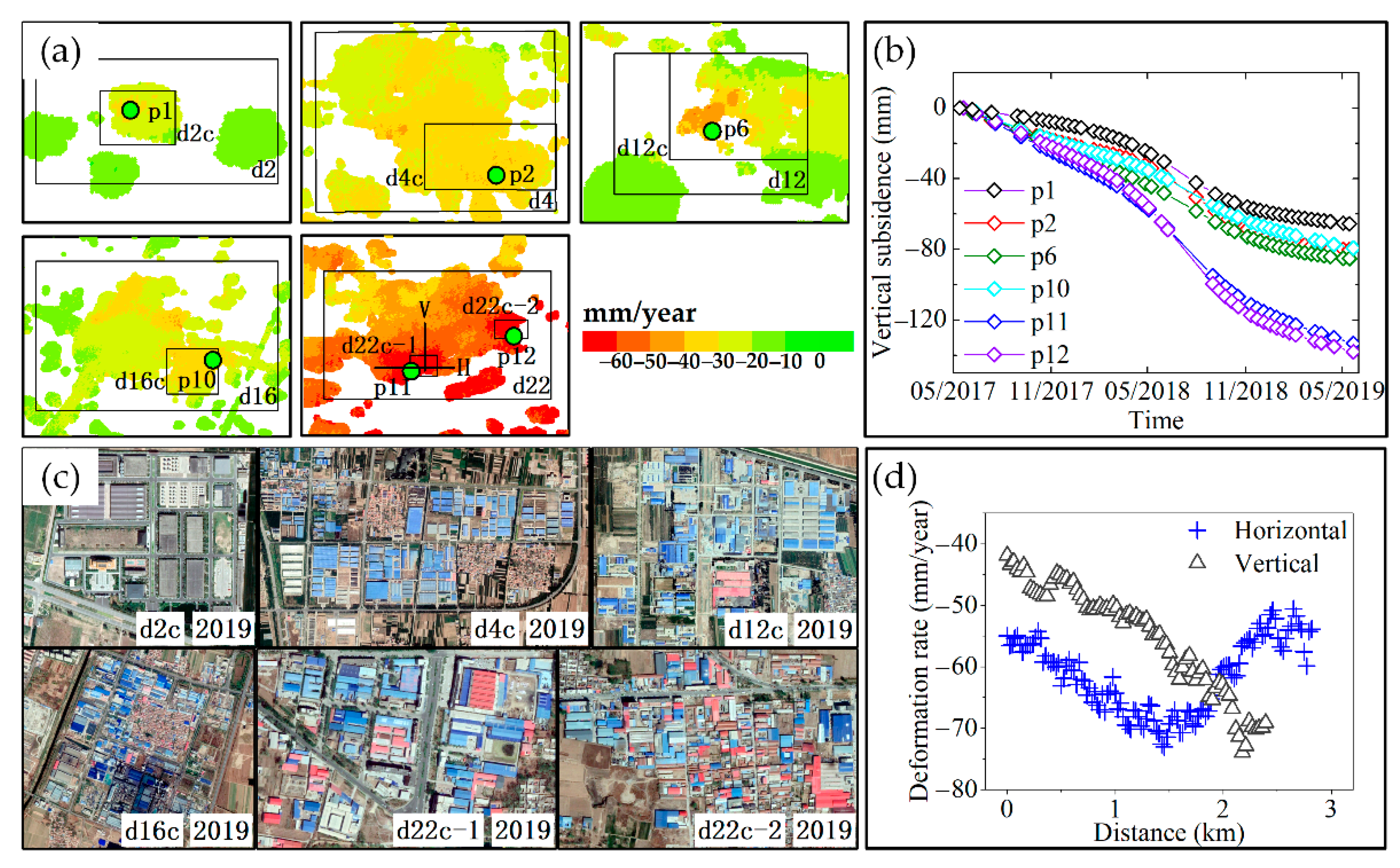
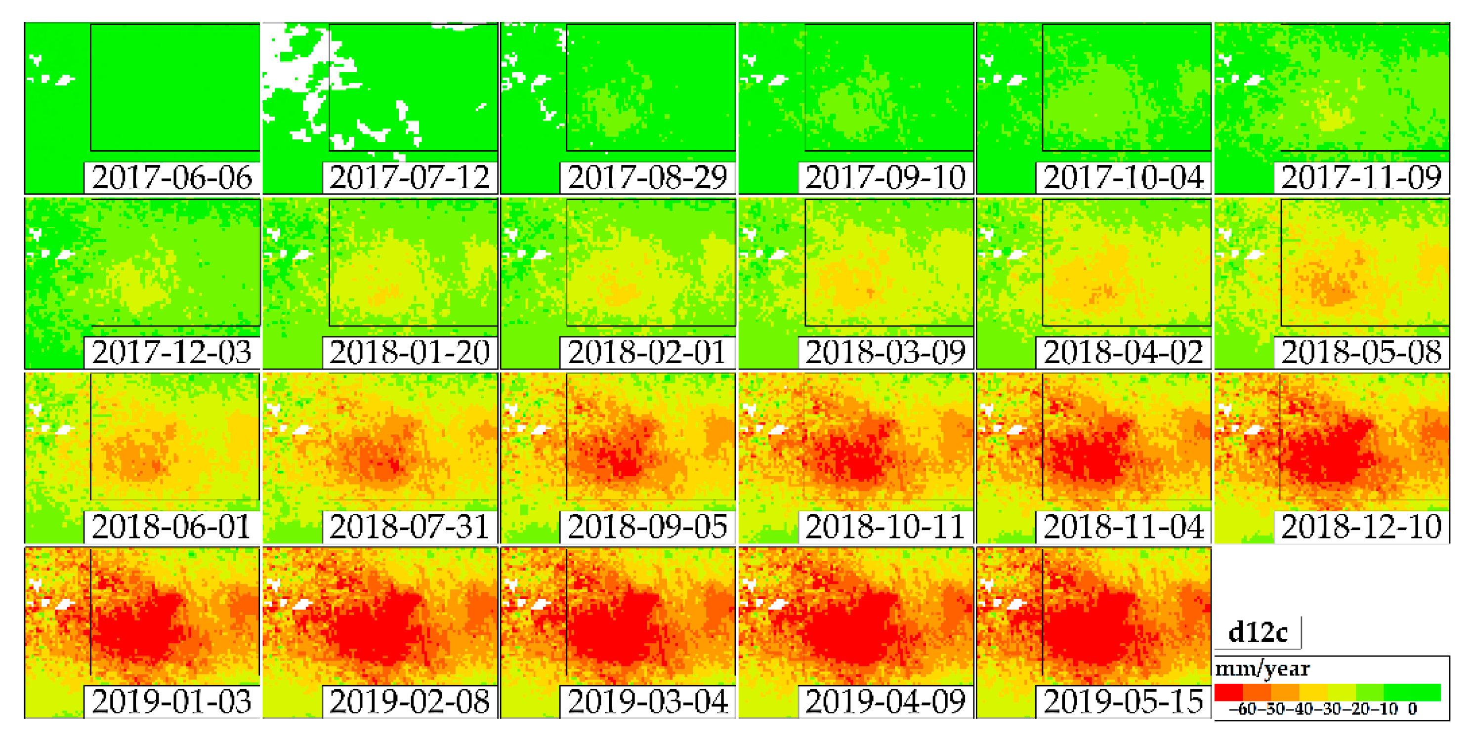
5.3. Industrial Areas and Land Subsidence

The land use may affect the groundwater balance and lead to the evolution of land subsidence [44]. As shown in Figure 18a, severe subsidence areas were mainly orange or red areas. Six remarkable subsidence bowl centers (d2c, d4c, d12c, d16c, d22c-1, and d22c-2) associated with industrial areas were found. The maximum subsidence velocity in d2c, d4c, d12c, d16c, and d22c reached around −36 mm/year, −48 mm/year, −50 mm/year, −45 mm/year, −48 mm/year, and −79 mm/year, respectively. Six feature points were extracted and their deformation time-series are given in Figure 18b. The subsidence bowl centers and the industrial areas were consistent to some extent, although the distribution range of the subsidence bowl centers were different from the industrial areas. Two groups of Google Earth images over six subsidence bowl centers (Figure 18c) acquired in 2019, respectively, show the details in the industrial area. Subsidence bowl d2c is located at the Congtai Liquor Factory, Feixiang Economic Development Zone of Handan City. It is suspected to be related to the large amount of water used for liquor making. Bowl center d4c is a gathering place of industrial areas, located in Zhaolizhuang Village of Quzhou County, Handan City. Bowl center d12c is located in Xinleitou Village of Xinji City, Shijiazhuang City, and there are 30 to 40 chemical fiber, filter paper, and food factories that require a lot of water. Figure 19 shows the accumulative time-series deformation of d12c. Bowl center d16c is located in Renhe Street and Guanzhou Road, Dongguang County of Cangzhou City. There are dozens of factory gathering areas in d16c, especially machinery factories, chemical factories, and plastic products. Bowl center d22c is located in Nansha Village and Yuejiazuo Village of Gaoyang County, Baoding City. Hundreds of companies gather in d22, especially textile companies related to oil exploration. Gaoyang County is known as the hometown of textiles, with textile enterprises accounting for 91.8%. The two horizontal and vertical deformations along the distance through the subsidence center d22c-1 are plotted in Figure 18d. In general, the larger the industrial plants, the more groundwater consumed for industrial production, leading to land subsidence. A relatively high spatial correlation also existed between locations of land subsidence bowls and industrial areas.

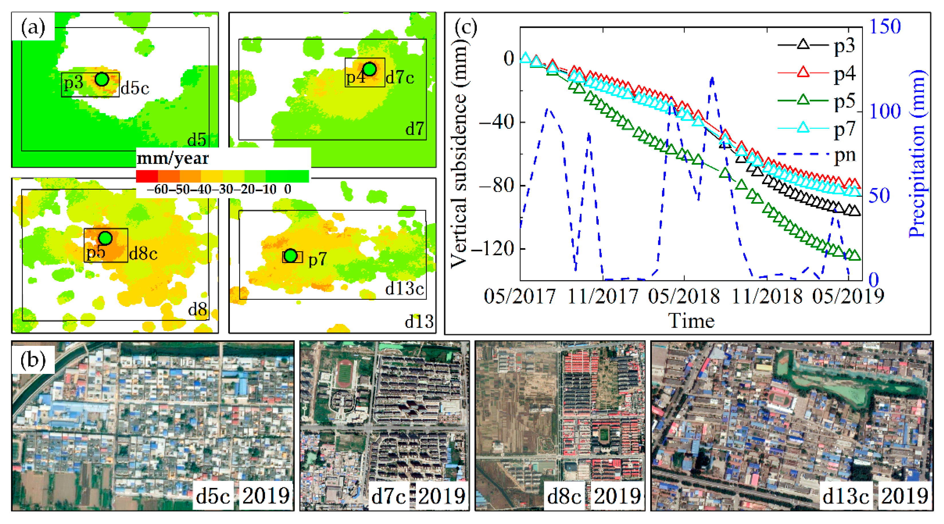
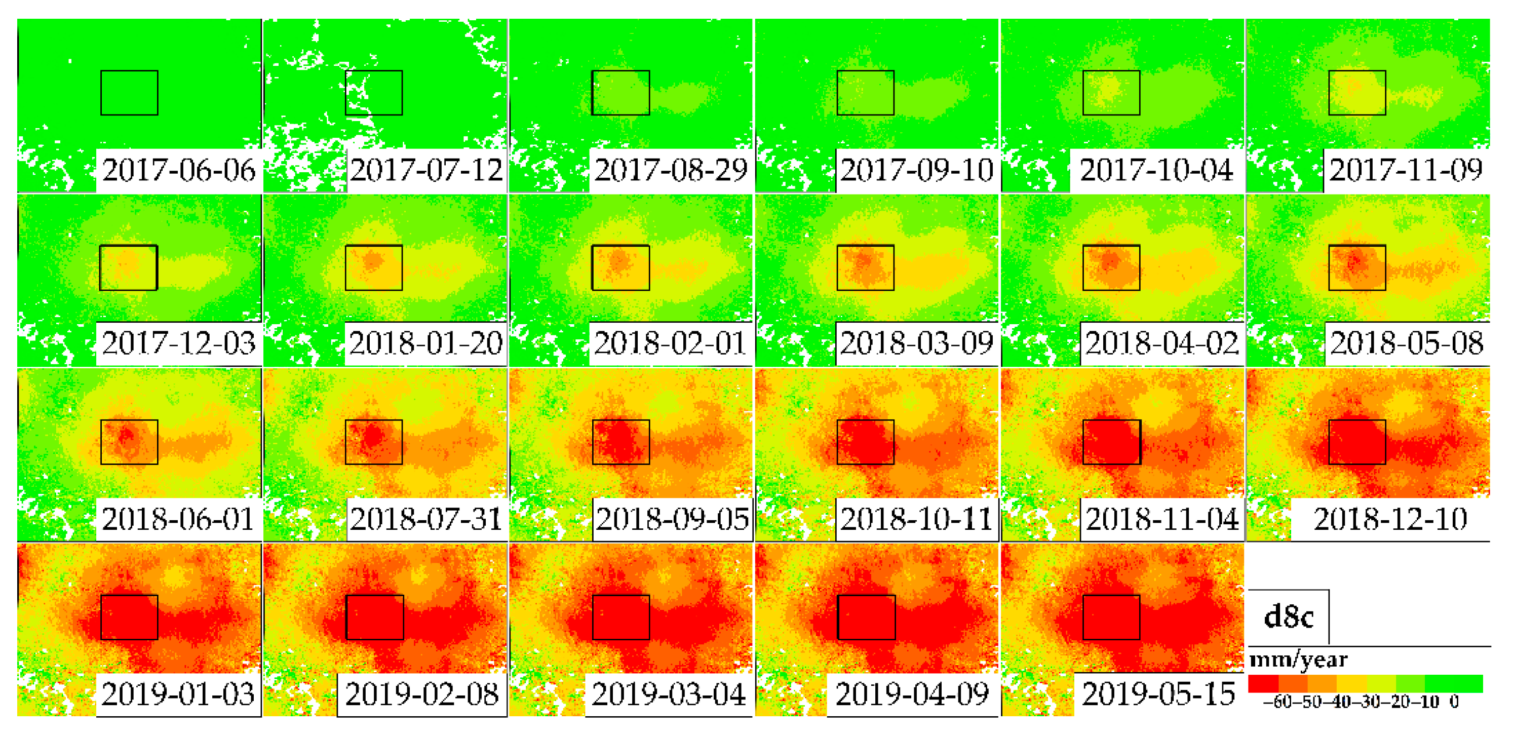
5.4. Dense Residential Areas and Land Subsidence

In addition, there a high spatial correlation exists between the locations of land subsidence bowls and dense residential areas. Figure 20a shows the deformation velocity map in the vertical direction in four subsidence bowls (d5, d7, d8, and d13) from May 2017 to May 2019. Four remarkable subsidence bowl centers (d5c, d7c, d8c, and d13c) associated with dense residential areas were successfully found. Google Earth images over four areas acquired in 2019 are shown in Figure 20b. The subsidence bowl center of d5 is located in Dawuzhuang, Xiangdu District of Xingtai City. Subsidence bowl center d7 is located in Shengfeng Times and Zhongxiadijingcheng in Wei County of Xingtai City. Subsidence bowl center d8 is located in the Shengshi Capital, Julu County of Xingtai City. Subsidence bowl center d13 is located in No. 195 Yongping Street, Hengshui City of Shenzhou City. To study the temporal deformation evolution, four feature points over four subsidence area were extracted and are given in Figure 20c. Figure 21 shows the accumulative time-series deformation of d12c. The maximum subsidence velocity in d5c, d7c, d8c, and d13c reached around −58 mm/year, −56 mm/year, −59 mm/year, and −51 mm/year, respectively. To sum up, land subsidence is highly consistent with dense residential areas.

Meanwhile, we analyzed subsidence with monthly precipitations acquired from the China Meteorological Data Service Center [56] from May 2017 to May 2019 at the p5 point. As we can see from Figure 20c, the precipitations declined noticeably from November 2017 to March 2018 and from September 2018 to March 2019 while subsidence velocity increased significantly. Precipitations were the highest from May 2017 to October 2017 and from April 2018 to August 2018 while the subsidence velocity slowed down slightly. All these phenomena suggest the following: that surface subsidence at the p5 point varies with the seasons and precipitation is one of the factors influencing land subsidence.

5.5. Faults and Land Subsidence

Figure 22a demonstrates a strong correlation between the land subsidence and fault distribution in the Hebei Plain, which indicates that the main deformation direction is basically parallel to the faults. From Figure 22a, a total of 21 subsidence bowls were distributed on both sides of the major faults. Figure 22b–d shows an example of the average subsidence velocity in three fault zones along profile aa’, bb’, and cc’. Sharp gradients in subsidence were observed across the faults, especially profile aa’ with subsidence gradients up to 40 mm/year. These high-velocity gradients correlate with faults, indicating that these faults coincide with the subsidence bowls.

6. Conclusions

Through using two TS-InSAR techniques, SBAS and NSBAS, we obtained a large-scale deformation map (about 45,000 km²) for Hebei Plain, with 166 Sentinel-1A data of tracks 40 and 142 from May 2017 to May 2019. We also identified 26 notable subsidence bowls in Handan, Xingtai, Shijiazhuang, Hengshui, Cangzhou, and Baoding, with maximum subsidence rates of −65 mm/year, −71 mm/year, −50 mm/year, −62 mm/year, −54 mm/year, and −79 mm/year, respectively. Subsidence bowls tend to be connected in the administrative area. A novel data fusion flow for the generation of land subsidence vertical velocity of adjacent-track was proposed, named FTASA. In addition, this method does not need to interpolate and correct the PS point, which further reduces the error and improves the accuracy. FTASA was successfully applied to the deformation monitoring in the Hebei Plain. FTASA had a higher accuracy than FO. The InSAR results with leveling measurements show good agreement with a precision of 9 mm/year. The InSAR results within tracks 40 and 142 and benchmark on the bedrock results also had a good correlation. The standard deviation of the InSAR results velocity calculated between tracks 40 and 142 was 7.37 mm/year. The correlation coefficient of track 40 and 142 was 0.89.

We found that eight subsidence bowls were positively correlated with Ningbolong and Gaoliqing-Sunin shallow groundwater funnels and Nangong deep groundwater funnel. Furthermore, we found that three, five, four, and three subsidence bowls were positively correlated with building constructions, industrial areas, dense residential areas, and faults, respectively. In our future work, we will try to combine change detection by using deep learning to analyze the influence of changes in different land types on the deformation results. A more detailed summary and future work are as follows:

• The land subsidence bowls have a positive correlation with the shallow or deep groundwater funnels. We found that there were six ground subsidence bowls in the shallow ground-water funnel, and two ground subsidence bowls in the deep groundwater funnel. In the future, the mechanisms underlying groundwater-induced land surface displacement deserves further analysis.
• Building constructions increase surface loads, aggravating land subsidence. Three remarkable subsidence bowl centers associated with building construction were successfully detected. For the first time, we tried to analyze the subsidence causes from the perspective of change detection in the Hebei Plain. Whether it is the load of the building that provokes the subsidence, or the required groundwater pumping to have a dry environment to build the foundations of those buildings, the subsidence mechanism needs to be further studied.
• Six remarkable subsidence bowl centers associated with an industrial area were found. The larger the industrial plants, the more groundwater consumed for industrial production, leading to land subsidence. A relatively high spatial correlation also existed between locations of land subsidence bowls and industrial areas.
• A high spatial correlation existed between the locations of four land subsidence bowls and dense residential areas. Precipitation was one of the factors influencing land subsidence. We can analyze the causes of land subsidence from the hydrogeological properties of rocks in our future work.
• There was a strong correlation between three land subsidence and fault distributions where the main deformation direction is basically parallel to the faults. A total of 21 subsidence bowls were distributed on both sides of major faults. These high-velocity gradients correlate with faults in three subsidence bowls, indicating that these faults coincide with the subsidence bowls.

References

1. Galloway, D.L.; Burbey, T.J. Review: Regional land subsidence accompanying groundwater extraction. Hydrogeol. J. 2011, 19, 1459–1486. [Google Scholar] [CrossRef]
2. Cigna, F.; Tapete, D. Satellite InSAR survey of structurally controlled land subsidence due to groundwater exploitation in the Aguascalientes Valley, Mexico. Remote Sens. Environ. 2021, 254, 112254. [Google Scholar] [CrossRef]
3. Mahmoudpour, M.; Khamehchiyan, M.; Nikudel, M.R.; Ghassemi, M.R. Characterization of Regional Land Subsidence Induced by Groundwater Withdrawals in Tehran, Iran. Geopersia 2013, 3, 49–62. [Google Scholar]
4. Erkens, G.; Bucx, T.; Dam, R.; De Lange, G.; Lambert, J. Sinking Coastal Cities. In Proceedings of the International Association of Hydrological Sciences, Nagoya, Japan, 15–19 November 2015. [Google Scholar]
5. Guzy, A.; Malinowska, A.A. State of the art and recent advancements in the modelling of land subsidence induced by groundwater withdrawal. Water 2020, 12, 2051. [Google Scholar] [CrossRef]
6. Yang, Y.; Luo, Y.; Liu, M.; Wang, R.; Wang, H. Research of Features Related to Land Subsidence and Ground Fissure Disasters in the Beijing Plain. In Proceedings of the International Association of Hydrological Sciences, Nagoya, Japan, 15–19 November 2015. [Google Scholar]
7. Gong, H.; Pan, Y.; Zheng, L.; Li, X.; Zhu, L.; Zhang, C.; Huang, Z.; Li, Z.; Wang, H.; Zhou, C. Long-term groundwater storage changes and land subsidence development in the North China Plain (1971–2015). Hydrogeol. J. 2018, 26, 1417–1427. [Google Scholar] [CrossRef] [Green Version]
8. Guo, H.; Zhang, Z.; Cheng, G.; Li, W.; Li, T.; Jiao, J.J. Groundwater-derived land subsidence in the North China Plain. Environ. Earth Sci. 2015, 74, 1415–1427. [Google Scholar] [CrossRef]
9. Yang, Y. Land Subsidence Disaster Prevention and Cure in Beijing-Tianjin-Hebei Area, China. Urban Geol. 2015, 1, 1–7. [Google Scholar]
10. Tang, Q.; Zhang, X.; Tang, Y. Anthropogenic impacts on mass change in North China. Geophys. Res. Lett. 2013, 40, 3924–3928. [Google Scholar] [CrossRef]
11. Zhang, J.; Chu, L.; Xiao, Z.; Lu, Z.; Shen, R.; Chen, Y. Main progress and achievements of land subsidence survey and monitoring in Hebei Plain. Geol. Surv. China. 2014, 1, 45–50. [Google Scholar]
12. Ge, Y. Impacts of Crop Production on Groundwater Depletion in the Hebei Plain. Master’s Thesis, Tsinghua University, Beijing, China, 2 June 2017. [Google Scholar]
13. Liu, Y.; Li, Y.; Jin, X.; Ma, B. Analysis of groundwater dynamics and influencing factors in Hebei Plain during the “Eleventh Five-Year Plan”. Groundwater 2015, 37, 52–55. [Google Scholar]
14. Li, Z. Characteristics and mechanism of land subsidence in Hebei Plain. Ph.D. Thesis, China University of Geosciences, Beijing, China, 6 June 2012. [Google Scholar]
15. Zhao, Q.; Zhang, B.; Yao, Y.; Wu, W.; Meng, G.; Chen, Q. Geodetic and hydrological measurements reveal therecent acceleration of groundwater depletion in North China Plain. J. Hydrol. 2019, 575, 1065–1072. [Google Scholar] [CrossRef]
16. Shi, M.; Gong, H.; Gao, M.; Chen, B.; Zhang, S.; Zhou, C. Recent Ground Subsidence in the North China Plain, China, Revealed by Sentinel-1A Datasets. Remote Sens. 2020, 12, 3579. [Google Scholar] [CrossRef]
17. Zhou, H.; Wang, Y.; Yan, S.; Wu, Y.; Liu, Q. Land subsidence monitoring and analyzing of Cangzhou area Sentinel-1A/B based time-series InSAR. Bull Surv. Map. 2017, 7, 89–93. [Google Scholar]
18. Gabriel, A.K.; Goldstein, R.M.; Zebker, H.A. Mapping small elevation changes over large areas: Differential radar interferometry. J. Geophys. Res. Atmos. 1989, 94, 9183–9191. [Google Scholar] [CrossRef]
19. Crosetto, M.; Monserrat, O.; Cuevas-González, M.; Devanthéry, N.; Crippa, B. Persistent scatterer interferometry: A review. ISPRS J. Photogramm. Remote. Sens. 2015, 115, 78–89. [Google Scholar] [CrossRef] [Green Version]
20. Galloway, D.L.; Hudnut, K.W.; Ingebritsen, S.E.; Phillips, S.P.; Peltzer, G.; Rogez, F.; Rosen, P.A. Detection of aquifer system compaction and land subsidence using interferometric synthetic aperture radar, Antelope Valley, Mojave Desert, California. Water Resour. Res. 1998, 34, 2573–2585. [Google Scholar] [CrossRef]
21. Hanssen, R.F. Radar Interferometry: Data Interpretation and Error Analysis; Springer Science & Business Media: Berlin, Germany, 2001. [Google Scholar]
22. Berardino, P.; Fornaro, G.; Lanari, R.; Sansoto, E. A new algorithm for surface deformation monitoring based on small baseline differential SAR interferograms. IEEE Trans. Geosci. Remote Sens. 2002, 40, 2375–2383. [Google Scholar] [CrossRef] [Green Version]
23. Ferretti, A.; Prati, C.; Rocca, F. Permanent scatterers in SAR interferometry. IEEE Trans. Geosci. Remote Sens. 2001, 39, 8–20. [Google Scholar] [CrossRef]
24. Ferretti, A.; Prati, C.; Rocca, F. Nonlinear subsidence rate estimation using permanent scatterers in differential SAR interferometry. IEEE Trans. Geosci. Remote Sens. 2000, 38, 2202–2212. [Google Scholar] [CrossRef] [Green Version]
25. Wang, Y.; Yang, Z.; Li, Z.; Zhu, J.; Wu, L. Fusing adjacent-track InSAR datasets to densify the temporal resolution of time-series 3-D displacement estimation over mining areas with a prior deformation model and a generalized weighting least-squares method. J. Geod. 2020, 94, 1–17. [Google Scholar] [CrossRef]
26. Tong, X.; Liu, S.; Li, R.; Xie, H.; Liu, S.; Qiao, G.; Feng, T.; Tian, Y.; Zhen, Y. Multi-track extraction of two-dimensional surface velocity by the combined use of differential and multiple-aperture InSAR in the Amery Ice Shelf, East Antarctica. Remote Sens. Environ. 2018, 204, 122–137. [Google Scholar] [CrossRef]
27. Samsonov, S.; Oreye, N.; González, P.; Tiampo, K.; Ertolahti, L.; Clague, J. Rapidly accelerating subsidence in the Greater Vancouver region from two decades of ERS-ENVISAT-RADARSAT-2 DInSAR measurements. Remote Sens. Environ. 2014, 143, 180–191. [Google Scholar] [CrossRef] [Green Version]
28. Zhao, Q.; Ma, G.; Wang, Q.; Yang, T.; Liu, M.; Gao, W.; Falabella, F.; Mastro, P.; Pepe, A. Generation of long-term InSAR ground displacement time-series through a novel multi-sensor data merging technique: The case study of the Shanghai coastal area. ISPRS J. Photogramm. Remote Sens. 2019, 154, 10–27. [Google Scholar] [CrossRef]
29. Ketelaar, G.; Leijen, F.; Marinkovic, P.; Hanssen, R. Multi-track PS-InSAR datum connection. In Proceedings of the IEEE International Geoscience and Remote Sensing Symposium, Barcelona, Spain, 23–27 July 2007. [Google Scholar]
30. Perissin, D.; Prati, C.; Rocca, F. ASAR Parallel-track PS Analysis in Urban Sites. In Proceedings of the IEEE International Geoscience and Remote Sensing Symposium, Barcelona, Spain, 23–27 July 2007. [Google Scholar]
31. Zhao, C.; Liu, C.; Zhang, Q.; Lu, Z.; Yang, C. Deformation of Linfen-Yuncheng Basin (China) and its mechanisms revealed by Π-RATE InSAR technique. Remote Sens. Environ. 2018, 218, 221–230. [Google Scholar] [CrossRef]
32. Hong, S.; Wdowinski, S. Multitemporal multitrack monitoring of wetland water levels in the Florida Everglades using ALOS PALSAR data with interferometric processing. IEEE Geosci. Remote Sens. Lett. 2014, 11, 1355–1359. [Google Scholar] [CrossRef]
33. Pepe, A.; Bonano, M.; Zhao, Q.; Yang, T.; Wang, H. The Use of C-/X-Band Time-Gapped SAR Data and Geotechnical Models for the Study of Shanghai’s Ocean-Reclaimed Lands through the SBAS-DInSAR Technique. Remote Sens. 2016, 8, 911. [Google Scholar] [CrossRef] [Green Version]
34. Duan, L.; Gong, H.; Chen, B.; Zhou, C.; Lei, K.; Gao, M.; Yu, H.; Cao, Q.; Cao, J. An Improved Multi-Sensor MTI Time-Series Fusion Method to Monitor the Subsidence of Beijing Subway Network during the Past 15 Years. Remote Sens. 2020, 12, 2125. [Google Scholar] [CrossRef]
35. Wang, H.; Wright, T.; Yu, Y.; Lin, H.; Jiang, L.; Li, C.; Qiu, G. InSAR reveals coastal subsidence in the Pearl River Delta, China. Geophys. J. Int. 2012, 191, 1119–1128. [Google Scholar] [CrossRef] [Green Version]
36. Sun, H.; Zhang, Q.; Zhao, C.; Yang, C.; Sun, Q.; Chen, W. Monitoring land subsidence in the southern part of the lower Liaohe plain, China with a multi-track PS-InSAR technique. Remote Sens. Environ. 2017, 188, 73–84. [Google Scholar] [CrossRef] [Green Version]
37. Du, Y.; Feng, G.; Liu, L.; Fu, H.; Peng, X.; Wen, D. Understanding Land Subsidence Along the Coastal Areas of Guangdong, China, by Analyzing Multi-Track MTInSAR Data. Remote Sens. 2020, 12, 299. [Google Scholar] [CrossRef] [Green Version]
38. Shirzaei, M. A seamless multitrack multitemporal InSAR algorithm. Geochem. Geophys. Geosyst. 2015, 16, 1656–1669. [Google Scholar] [CrossRef]
39. Jiang, L.; Bai, L.; Zhao, Y.; Cao, G.; Wang, H.; Sun, Q. Combining InSAR and hydraulic head measurements to estimate aquifer parameters and storage variations of confined aquifer system in Cangzhou, North China Plain. Water Resour. Res. 2018, 54, 8234–8252. [Google Scholar] [CrossRef]
40. Ge, D.Q.; Wang, Y.; Guo, X.F.; Fan, J.H.; Liu, S.W. Surface deformation field monitoring by use of small-baseline differential interferograms stack. J. Geod. Geodyn. 2008, 28, 61–66. [Google Scholar]
41. Ge, D.Q.; Wang, Y.; Guo, X.F.; Liu, S.W.; Fan, J.H. Surface deformation monitoring with multi-baseline D-InSAR based on coherent point target. J. Remote Sens. 2007, 11, 574–580. [Google Scholar]
42. Zhang, Y.; Wu, H.; Kang, Y.; Zhu, C. Ground Subsidence in the Beijing-Tianjin-Hebei Region from 1992 to 2014 Revealed by Multiple SAR Stacks. Remote Sens. 2016, 8, 675. [Google Scholar] [CrossRef] [Green Version]
43. Duan, W.; Zhang, H.; Wang, C.; Tang, Y. Multi-Temporal InSAR Parallel Processing for Sentinel-1 Large-Scale Surface Deformation Mapping. Remote Sens. 2020, 12, 3749. [Google Scholar] [CrossRef]
44. Zhou, C.; Gong, H.; Chen, B.; Gao, M.; Cao, Q.; Cao, J.; Duan, L.; Zuo, J.; Shi, M. Land Subsidence Response to Different Land Use Types and Water Resource Utilization in Beijing-Tianjin-Hebei, China. Remote Sens. 2020, 12, 457. [Google Scholar] [CrossRef] [Green Version]
45. Samsonov, S.; van der Kooij, M.; Tiampo, K. A simultaneous inversion for deformation rates and topographic errors of DInSAR data utilizing linear least square inversion technique. Comput. Geosci. 2011, 37, 1083–1091. [Google Scholar] [CrossRef]
46. Department of Water Resources of Hebei Province. Hebei Water Resources Bulletin 2019. Available online: http://slt.hebei.gov.cn/resources/43/202010/1603098695816085596.pdf (accessed on 6 September 2020).
47. Department of Water Resources of Hebei Province. Hebei Water Resources Bulletin 2018. Available online: http://slt.hebei.gov.cn/resources/43/201909/1568618211289023678.pdf (accessed on 28 October 2020).
48. Copernicus. Copernicus Open Access Hub. Available online: https://scihub.copernicus.eu/ (accessed on 8 September 2019).
49. Sentinel-1 Quality Control. POD Precise Orbit Ephemerides. Available online: https://qc.sentinel1.eo.esa.int/ (accessed on 8 September 2019).
50. Lopez-Quiroz, P.; Doin, M.; Tupin, F.; Briole, P.; Nicolas, J. Time-series analysis of Mexico City subsidence constrained by radar interferometry. J. Appl. Geophys. 2009, 69, 1–15. [Google Scholar] [CrossRef]
51. Jolivet, R.; Lasserre, C.; Doin, M.; Guillaso, S.; Peltzer, G.; Dailu, R.; Sun, J.; Shen, Z.; Xu, X. Shallow creep on the Haiyuan Fault (Gansu, China) revealed by SAR Interferometry. J. Geophys. Res. Solid Earth. 2012, 117, B06401. [Google Scholar] [CrossRef] [Green Version]
52. Doin, M.; Lodge, F.; Guillaso, S.; Jolivet, R.; Lasserre, C.; Ducret, G.; Grandin, R.; Pathier, E.; Pinel, V. Presentation of the small baseline NSBAS processing chain on a case example: The Etna deformation monitoring from 2003 to 2010 using Envisat data. Proceedings the of Fringe Esa Conference, Frascati, Italy, 19–23 September 2011. [Google Scholar]
53. Agram, P.; Jolivet, R.; Riel, B.; Lin, Y.N.; Simons, M.; Hetland, E.; Doin, M.-P.; Lasserre, C. New Radar Interferometric Time-series Analysis Toolbox Released. Eos Trans. Am. Geophys. Union 2013, 94, 69–70. [Google Scholar] [CrossRef] [Green Version]
54. Earthdef. Generic InSAR Analysis Toolbox (GIAnT)—User Guide. 2012. Available online: http://earthdef.caltech.edu (accessed on 6 September 2020).
55. Lin, Y.; Simons, M.; Hetland, E.; Muse, P.; DiCaprio, C. A multiscale approach to estimating topographically correlated propagation delays in radar interferograms. Geochem. Geophys. Geosyst. 2010, 11. [Google Scholar] [CrossRef]
56. CMDC. China Meteorological Data Service Centre. Available online: http://data.cma.cn (accessed on 18 September 2020).
Figure 1. Hazards of land subsidence in Hebei Plain. (a,b) The Cangzhou People’s Hospital sank due to land subsidence. (c) Water accumulation caused by land subsidence in Cangzhou; (d) The Putong Temple tower skew caused by land subsidence in Nangong County, Xingtai City (provided by Hebei Geo-Environment Monitoring).
Remotesensing 13 00795 g001
Figure 2. Study area and coverage of SAR data tracks superimposed on one arc-second Shuttle Radar Topography Mission (SRTM) digital elevation model (DEM) shaded topography map over Hebei Plain, China. The right-top inset is the location of Hebei Province in China and the blue border is Hebei Province. Dark amethyst and fir green rectangles are the Sentinel-1A tracks 40 and 142 coverage, respectively. Red border is the study area. The six bench marks are marked with black triangles and the two benchmarks on the bedrock are marked with a black cross.
Remotesensing 13 00795 g002
Figure 3. Shallow groundwater depth in the plain area of Hebei Pin 2018 and 2019 (adapted from [46,47]).
Remotesensing 13 00795 g003
Figure 4. List of Sentinel-1A SAR data. Fir green and black cycles indicate the track 40 data list and track 142 data list, respectively.
Remotesensing 13 00795 g004
Figure 5. Flowchart of FTASA.
Remotesensing 13 00795 g005
Figure 6. Images of pre-registration and post-registration. The lighter section above the line is the amplitude image of track 40, and the darker section below the line is the amplitude image of track 142. Two delft blue ellipses show the effect of pre-registration and post-registration of tracks 40 and 142. (a) Pre-registration comparison chart of tracks 40 and 142; (b) Post-registration comparison chart of tracks 40 and 142.
Remotesensing 13 00795 g006
Figure 7. Combined singular value decomposition (SVD) solution of the deformation time-series results of the adjacent-track in an overlapping area. The bottom images are the partial deformation time-series results. The abscissa represents time and the ordinate represents two adjacent-tracks.
Remotesensing 13 00795 g007
Figure 8. Mean vertical displacement velocities generated by TS-InSAR techniques from May 2017 to May 2019. The black line is the overlapping area of tracks 40 and 142. (a) Vertical deformation velocity of tracks 40 calculated by SBAS; (b) Vertical deformation velocity of track 142 calculated by SBAS; (c) Vertical deformation velocity of track 40 calculated by NSBAS; (d) Vertical deformation velocity of track 142 calculated by NSBAS.
Remotesensing 13 00795 g008
Figure 9. Mean vertical displacement velocities map of Hebei Plain involving seven cities. Amethyst rectangles are representative of 26 subsidence bowls, named from d0 to d25. The four X marks (AD) are the validation points of tracks 40 and 142.
Remotesensing 13 00795 g009
Figure 10. Distribution of 26 subsidence bowls in seven administrative zones. The six color and corresponding numbers stand for different administrative labelled with the total bowl numbers. Bold black line is our study area. Light black lines are the seven administrative zones.
Remotesensing 13 00795 g010
Figure 11. Vertical deformation velocity in FO, FTASA, and leveling. The black stars are the leveling results. The blue crosses are the FTASA results, and the black triangles are the FO results.
Remotesensing 13 00795 g011
Figure 12. Difference of the corresponding PS points of vertical deformation velocity between FTASA and FO.
Remotesensing 13 00795 g012
Figure 13. Comparison between the InSAR results and leveling results from May 2017 to May 2019, and the comparison between InSAR results and benchmark on bedrock results from December 2017 to June 2018. The black stars are the leveling results, the black cycles are the benchmark on bedrock results, and the blue crosses are the InSAR results. The location of the benchmark is shown in Figure 2.
Remotesensing 13 00795 g013
Figure 14. The accuracy of the deformation results of tracks 40 and 142. (a) Blue bars represent the histograms of vertical deformation velocity difference in the overlapping region of tracks 40 and 142. The standard deviation was 7.37 mm/year; (b) The linear fitting results between tracks 40 and 142 of the overlapping area. The blue color represents the vertical deformation velocity, and the black line represents the linear fitting function. The linear fitting formula is shown in the figure.
Remotesensing 13 00795 g014
Figure 15. Deformation time-series at four points (A–D) derived from the Sentinel-1A of tracks 40 and 142 from May 2015 to May 2019 (ad). The four points (A–D) are marked in Figure 9. Black circle represents track 40 and the green circle represents track 142.
Remotesensing 13 00795 g015
Figure 16. The range of groundwater funnels and the distribution of land subsidence bowls. The areas of amethyst cycle and blue cycle are the areas of the groundwater funnels in 2018 and 2019, respectively. The groundwater depth contours have been marked on both sides of the line. (a,b) Amethyst and blue octagon represent the shallow groundwater funnels center in 2018 and 2019, respectively. (c) The Nangong deep groundwater funnel center in 2018 and 2019 is represented by the green octagon.
Remotesensing 13 00795 g016
Figure 17. (a) Mean vertical displacement velocities in subsidence bowl centers d0c, d14c, and d15c; (b) Land coverage maps of d0c, d14c, and d15c in May 2017 and May 2019. The images are from Google Earth. These subsidences are related to expansion or the demolition of buildings; (c) Accumulative time-series subsidence in p0, p8, and p9 points from May 2017 to May 2019.
Remotesensing 13 00795 g017
Figure 18. (a) Mean vertical displacement velocities of d2c, d4c, d12c, d16c, d22-1c, d22-2c; (b) The accumulative time-series subsidence of p1, p2, p6, p10, p11, and p12 points from May 2017 to May 2019; (c) Land coverage maps of d2c, d4c, d12c, d16c, d22c-1, and d22c-2 from May 2017 to May 2019. The images are from Google Earth. These subsidence are related to industrial clusters; (d) Horizontal and vertical subsidence (shown in (a)) of bowl center d22c-1.
Remotesensing 13 00795 g018
Figure 19. Accumulative time-series subsidence of d12c from May 2017 to May 2019 (only the partial time-series selected by the month).
Remotesensing 13 00795 g019
Figure 20. (a) Mean vertical displacement velocities of d5c, d7c, d8c, and d13c. (b) Land coverage maps of d5c, d7c, d8c, and d13c in 2019. The images are from Google Earth. These subsidences are related to dense residential areas; (c) Accumulative time-series subsidence of p3, p4, p5, and p7 points from May 2017 to May 2019, and monthly precipitation at the p5 point.
Remotesensing 13 00795 g020
Figure 21. Accumulative time-series subsidence of bowl center d8c from 2017 to 2019 (only the partial time-series selected by the month).
Remotesensing 13 00795 g021
Figure 22. Land subsidence rate map in the Hebei Plain with some main faults. (a) Land subsidence velocity map, and blue dotted lines are faults; (bd) Deformation rates along profiles aa’, bb’, and cc’ in (bd), and the positions of aa’, bb’, and cc’ are labeled in (a).
Remotesensing 13 00795 g022