Technical Note

Application of Denoising CNN for Noise Suppression and Weak Signal Extraction of Lunar Penetrating Radar Data

1
College of Geo-Exploration Science and Technology, Jilin University, Changchun 130026, China
2
Science and Technology on Near-Surface Detection Laboratory, Wuxi 214035, China
3
Key Laboratory of Geophysical Exploration Equipment, Ministry of Education, Jilin University, Changchun 130026, China
*
Author to whom correspondence should be addressed.
Remote Sens. 2021, 13(4), 779; https://doi.org/10.3390/rs13040779
Submission received: 19 January 2021 / Revised: 13 February 2021 / Accepted: 18 February 2021 / Published: 20 February 2021
(This article belongs to the Special Issue Lunar Remote Sensing and Applications)

Abstract

:
As one of the main payloads mounted on the Yutu-2 rover of Chang’E-4 probe, lunar penetrating radar (LPR) aims to map the subsurface structure in the Von Kármán crater. The field LPR data are generally masked by clutters and noises of large quantities. To solve the noise interference, dozens of filtering methods have been applied to LPR data. However, these methods have their limitations, so noise suppression is still a tough issue worth studying. In this article, the denoising convolutional neural network (CNN) framework is applied to the noise suppression and weak signal extraction of 500 MHz LPR data. The results verify that the low-frequency clutters embedded in the LPR data mainly came from the instrument system of the Yutu rover. Besides, compared with the classic band-pass filter and the mean filter, the CNN filter has better performance when dealing with noise interference and weak signal extraction; compared with Kirchhoff migration, it can provide original high-quality radargram with diffraction information. Based on the high-quality radargram provided by the CNN filter, the subsurface sandwich structure is revealed and the weak signals from three sub-layers within the paleo-regolith are extracted.

Graphical Abstract

1. Introduction

After China’s Chang’E-3 (CE-3) mission was completed, the Chang’E-4 (CE-4) probe was launched on 8 December 2018, and achieved the first-ever soft landing on the farside of the moon on January 3, 2019. The landing site of CE-4 is on the floor of Von Kármán crater in the South Pole-Aitken (SPA) basin [1]. With a diameter of approximately 2500 km and the deepest depth of 13 km, the SPA basin is the largest impact structure on the moon and can provide important clues to the internal structure of the moon [2,3,4,5,6,7]. Recent works indicate that the near-surface materials measured by the CE-4 rover were mainly the ejecta from the Finsen crater, with possible contributions from the Alder, the Von Kármán L, and the Von Kármán L’ craters [7,8,9,10,11,12,13,14,15,16,17]. It is also convincing that the ejecta from the Finsen crater probably contains the lunar mantle materials [18,19,20,21].
The Yutu-2 rover, carried by CE-4, is mounted with a lunar penetrating radar (LPR) which is used to detect the lunar subsurface structure [22]. Similar to CE-3 [23,24], the LPR possesses two channels (CH-1 and CH-2) with center frequencies of 60 and 500 MHz, respectively [23,24,25,26,27,28,29]. The CH-2 consists of one transmitting antenna and two receiving antennas (also known as CH-2A and CH-2B) of different offsets [30,31,32]. The mission of CH-2 is to map the fine structure of the lunar regolith [23,24,25,26,27,28,29,30,31,32].
The CH-2 LPR amplitude-modulated and frequency-modulated signals are always masked by clutters and noises of large quantity [33]. The clutters with relatively low frequency may generate from the coupling of antennas and the instrument system, as there are many kinds of payloads mounted on the rover [22]. The processing of LPR data is challenging especially in noise suppression. In previous researches, many filtering methods have been applied to LPR data, such as band-pass filtering [34], bi-dimensional empirical mode decomposition (BDEMD) [35], complete ensemble empirical mode decomposition (CEEMD) [36], mathematical morphology filtering [37], and variational mode decomposition (VMD) [38]. However, these methods have their limitations and cannot provide a satisfactory result. More importantly, due to the attenuation of electromagnetic waves, the signals of great depth are quite weak and immersed within the noises. The noises and weak signals are of similar amplitudes and frequencies and cannot be easily classified using traditional denoising methods. Therefore, it is of vital importance to develop a more effective filtering method for LPR data processing. Convolutional neural network (CNN) [39,40,41] is a type of deep learning network architecture that is widely applied to various fields. In 2017, Zhang et al. proposed a CNN model for image denoising [42,43]. The denoising CNN model innovatively removed the pooling layers from the initial CNN model, as pooling layers may erase the characteristics of high-frequency noise.
In this article, the denoising CNN framework is applied to CE-4 LPR data filtering. The low-frequency clutters used in the CNN training are extracted from CE-3 LPR data using the empirical mode decomposition (EMD) [44]. Therefore, the achievement of noise suppression can also verify that the low-frequency clutters embedded in the CE-4 are the same as that of CE-3 and are generated from the instrument system of the rover. Based on the well trained CNN filter, the low-frequency clutters and high-frequency noises are both suppressed in the field LPR profile and the weak signals in the deep are extracted. To illustrate the superiority of the CNN filter on noise suppression, a classic band-pass filter and a mean filter are respectively conducted as comparisons. For discussing the results of weak signal extraction, the combined methods of the band-pass filter and the mean filter as well as the combined methods of the band-pass filter and the Kirchhoff migration are respectively conducted as comparisons. Finally, based on the high-quality radargram provided by the CNN filter, the subsurface sandwich structure is revealed and the weak signals from three sub-layers within the paleo-regolith are extracted.

2. Materials and Methods

2.1. The Initial CH-2B LPR Data

The walking route for the Yutu-2 rover on the moon for the first 12 lunar days is shown in Figure 1a [11]. The curve is ~320 meters in length. A series of processing steps, including the traces amending, the traces selecting, the time lag adjustment, the attenuation compensation, and the background removal [10,11,25,26,27,28,29,30,31] (The details are in Table A1) are conducted to obtain the initial CH-2B profile. The original profile and its average frequency amplitude spectrum are respectively shown in Figure 1b,c. Considering that the center frequency of the CH-2B LPR signal is 500 MHz with a bandwidth of 450 MHz [23,24], the radargram in Figure 1b is masked by low-frequency clutters and high-frequency noises of large quantity. Simultaneously, as the signals from the deep are very weak and their amplitudes are similar to the noise, the signals below 400 ns are more severely affected by the noise interference and the reflections from the strata are invisible or hard to recognize. Therefore, the key point of this article is to suppress the noises and extract the deep weak signals.

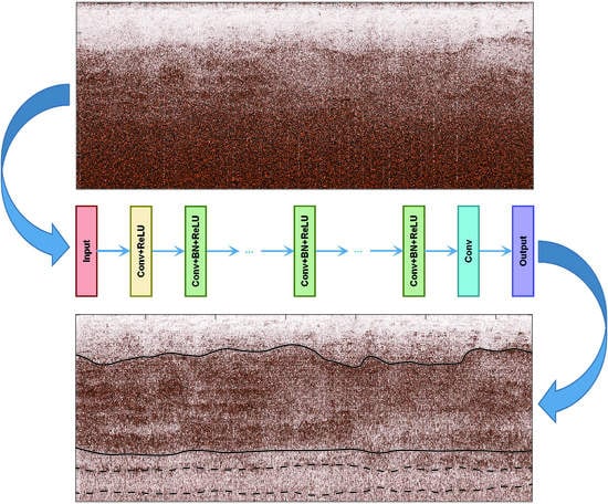
2.2. Methodology of Denoising CNN

The key idea of deep learning is to deepen the depth of the network for enhancing the accuracy of nonlinear matching. The CNN is a method of deep learning. It integrates the input data into a hierarchical stack of operations such as convolution operations, convergent operations, and nonlinear activation function mapping, and extracts features from the original data [39,40,41]. This process is called “feed-forward operation.” The last layer of the CNN compares the operation result with the target task, converts it into the objective function, obtains the error between the calculated value and the real value, and then uses the error back-propagation(BP) algorithm to propagate the error back. The error is assigned to the neurons of each layer, and then the parameters of each layer can be updated. This process is called “feed-back operation.” The iterations will continue until the objective function converges, which means the network is well trained. When new data are input, they can be predicted by the network’s feed-forward operation.
Denoising CNN is a CNN framework for image denoising. It innovatively removed the pooling layer from the initial CNN model. The framework of denoising CNN is shown in Figure 2 [42,43]. In this model, the batch normalization (BN) and the rectified linear unit (Relu) are applied. These two training techniques are used to avoid the vanishing gradient problem [42,43]. The mathematical form of BN is given by [42,43]:
P o u t = P i n mean ( P i n ) var ( P i n ) · γ + β ,
where Pin and Pout represent the input and output of a layer. Mean(Pin) and var(Pin) are the average value and standard deviation of Pin; γ and β are the learnable parameters.
The Relu is a type of nonlinear activation function widely applied in deep learning [42,43]. It always follows the convolutional layer, and its mathematical expression is shown as follow:
P o u t = max ( 0 , P i n · w + b ) ,
where w and b are the convolutional kernel and the threshold, respectively.

3. Results

3.1. CNN Training

The key of CNN training is to use the simulated GPR data with low-frequency clutters and high-frequency noises as the training data. The GPR simulations for different types of relative permittivity models are conducted using the finite-difference time-domain (FDTD) method. The models as well as their simulated data are shown in Figure 3a,b. The models contain different target combinations with different relative permittivity.
As we have discussed in Section 2.1, the LPR data are masked by low-frequency clutters and high-frequency noises of large quantities. The low-frequency clutter is considered to generate from the coupling of antennas and the instrument system, so it is relatively stable. As CE-4 is the backup of CE-3, we decide to extract 200 low-frequency clutters from CH-2B data of CE-3 using empirical mode decomposition (EMD) [44]. If the filtering result is satisfactory, the speculation for the source of low-frequency clutters can also be proved. The extracted clutters as well as their average frequency amplitude spectrum are respectively shown in Figure 4a,b. Besides, the high-frequency noise can be easily simulated by Gaussian noise. Subsequently, the low-frequency clutters and high-frequency noises are embedded into the simulated GPR data using the formula below:
I m a g e = L a b e l + α 1 L C + α 2 H N ,
where Label represents the simulated GPR data; LC and HN are low-frequency clutters and high-frequency noises, respectively; Image denotes the data masked by LC and HN. The α1 and α2 are the intensity coefficients. The greater α1 and α2 correspond to the lower signal-to-noise ratio (SNR).
Compared with the random noises, the clutters are more stable and, more importantly, time-related. Therefore, before adding clutters, the lengths of training radar profiles are re-sized into the length of clutters, which can make the training data remaining the features of clutters. Besides, the additions of LC are conducted for a single trace of the simulated data at a time. For each trace, we randomly draw one of the 200 clutters and add it to the signal.
Here, a test is conducted to determine the ranges of these two parameters in the CNN training process. The thresholds should contain most possible cases of different noise levels and the maximums of these two parameters should guarantee that the signals are almost immersed in clutters or noises. Besides, wider ranges of α1 and α2 will result in generating more training images which will decelerate the convergence of CNN training and make it more difficult and time-consuming. Therefore, we need to select the smallest ranges of α1 and α2 while covering most of the possible noise cases.
The tests with α1 = 0, 1, 1.5, and 2 and α2 = 0, 1, 3, and 5 are shown in Figure 5 and Figure 6, which are based on the simulated data of the first radargram in Figure 3b. It is evident that the signals from the target gradually become invisible with the increase in α1 and α2. To provide quantitative results, the image entropy is conducted for different images with different α1 and α2. The image entropy is given by [45,46,47]:
R = [ m = 1 M n = 1 N a 2 ( m , n ) ] 2 m = 1 M n = 1 N a 4 ( m , n ) ,
where M and N denote the vertical and horizontal size of a radar profile; a(m,n) represents the pixel value of the radargram at (m,n) position. This parameter is known to be an easily computable, accurate approximation to entropy [45,46,47]. The larger R value indicates the greater interference of clutters and noises.
Figure 7a shows the image entropy of the image with different α1 and α2; the blue and orange curves represent the clutters added and random noise added cases, respectively. Figure 7b presents the derivatives of the curves in Figure 7a. Both curves of image entropy rise with the increase in α1 and α2; when α1 = 2 and α2 = 5, the curves gradually become flat corresponding to the zero values of derivatives in Figure 7b. In this case, the clutters and noises become the main ingredients of the images. It is also feasible to keep increasing the α1 and α2, but the images will become complete clutters and noises without signals. These useless images will not strengthen the training result but make the training more time-consuming. Therefore, α1 ∈ [0, 2], α2 ∈ [0, 5] are reasonable thresholds that are the smallest and can cover most of the possible noise cases.
To expand the training data set and enhance the performance of CNN, the widely used data augmentation method [42,43] is subsequently applied. The augmentation contains horizontal and vertical flip. Finally, the augmented data are applied to the CNN training. The convergence curve of the loss function is shown in Figure 8. The objective function converges at approximately 200 iterations.

3.2. Model Denoising Test

In this section, the integrated model of lunar regolith [27,35] is applied to test the CNN filter. This model is built based on the actual environment of lunar regolith and stochastic media [27,35]. The relative permittivity model is shown in Figure 9. The top layer is a vacuum; the middle layer is the lunar regolith; the bottom layer is the bedrock. The grain sizes ascend with the increasing depth, due to the different weathering degree. The simulated GPR data, the noise embedded data, and the CNN filtering result are shown in Figure 10. The CNN filter can suppress both the low-frequency clutters and the high-frequency noise well. The filtered image is very close to the original image, the hyperbolas are well restored. Therefore, the results convince that the CNN for the GPR data denoising is feasible and the CNN model has been well trained. Besides, the signals in the radargram with both low-frequency clutter and high-frequency noises in Figure 10c are almost totally immersed in the interference and are hard to recognize. In the test, the amplitudes of the clutters and noises are set to be close to those of the signals, the case of which is similar to the field LPR data with the great depths. However, the CNN filter shows its stable ability to suppress the interference and restore the signals.

3.3. Denoising and Weak Signal Extraction of LPR Data

In this section, the well-trained denoising CNN model is applied to the denoising and weak signal extraction of LPR data. To well illustrate the superiority of the denoising CNN method, the classic band-pass filter is first conducted as the comparison method. The results of the band-pass filtering are shown in Figure 11a–c. The radargram contains much less noise compared to the initial radargram in Figure 1c which is also evident in the comparison of the average frequency amplitude spectra in Figure 11c. However, the signals below 400 ns are still masked with large quantities of noise and cannot be recognized. To explain the phenomenon, the S transformation [48] is conducted to analyze the property of the noise embedded in the LPR data after band-pass filtering. Four signals are extracted in Figure 11a and their S transformation results are presented in Figure 11d–g. It is obvious that the frequencies of the clutters and noises embedded below 400 ns are within the frequency band of LPR signals reflected from the subsurface structures and are also in the frequency band of the filter in Figure 11b. Therefore, the frequency-based filter such as the band-pass filter cannot suppress the clutter and noise below 400 ns.
This phenomenon can be interpreted to be the result of the magnification of the ringing effect and noise. Due to the attenuation of electromagnetic waves [29], the signals from the deep are weak and their amplitudes are close to the ringing signals. In order to make the deep signals more visible, the attenuation compensation [10,11,25,26,27,28,29,30,31] is necessary, resulting in the magnification of ringing signals and noise. This interference is of the same frequency band as the useful LPR signals and is difficult to suppress.
Subsequently, the CNN filter is applied to the LPR data. As a frequency-based filter such as the band-pass filter cannot suppress the clutter and noise below 400 ns, we simultaneously conducted the classical mean filter as a comparison method with the CNN filter. The mean filter is a typical linear filter, which involves a template to the target pixel on the image that includes the neighboring pixels around it (the 3 × 3 sized pixel region around the target pixel constitutes a filtering template). The filtering process removes the target pixel itself and replaces the original pixel value with the average of all the pixels in the template.
Figure 12a,b presents the results of the mean filter and CNN filter. Besides, Figure 12c,d shows the radargram after both band-pass and mean filtering and the radargram after both band-pass and Kirchhoff migration, respectively. For analyzing the processing results, Figure 12e compares the average frequency amplitude spectra of the results.
The result after only mean filtering cannot suppress the low-frequency clutter and high-frequency noise, which is also evident in the spectra comparison. As the purple curve in Figure 12e shows, the mean filter can suppress large quantities of high-frequency noises but the result is much worse than the CNN and band-pass filtering. Besides, the mean filtering has almost no attenuation ability for low frequency clutters.
The CNN filtering can suppress the clutters and noises well, especially for the signals below 400 ns (Figure 12b). An evident interface at ~500 ns and another unclear interface at ~600 ns can be found, which are pointed out by the double-way black arrows (Figure 12b). Furthermore, we test a combined method of conducting both the band-pass and the mean filters (Figure 12c). The CNN and the combined methods are similar in the spectra results, but the image quality of the combined method result falls flat. The imaging result of the combined method is still masked with many clutters and noises and only the unclear interface at ~500 ns can be observed whereas the signals at ~600 ns are immersed in the noise. Some strips of interference (the blue arrows in Figure 12c), which can also be observed in the original radargram (Figure 1a) or the mean filtering result (Figure 12a), are not completely removed. However, these interferences are well attenuated in the CNN filtering results. Therefore, the result of CNN filtering can present a radargram with higher quality compared with the combined method of band-pass and mean filtering.
Besides, the migration processing after band-pass filtering, which is commonly adopted in the previous studies [9,10,11], can present a similar result (Figure 12b) to that of the CNN filtering. However, the result of migration has attenuated the diffracted waves and is much more suitable for stratigraphic divisions [9,10,11] whereas the CNN filter can obtain an original radargram with the image of high quality and information of diffracted waves. The diffracted wave contains important information for property analysis of LPR data [30,32,34,37,38,49,50,51,52] and the high-quality image can guarantee the accuracy of the analysis. Overall, the result of migration can provide clues to stratigraphic divisions and the result of the CNN filter can provide high-quality radargram for property analysis.

3.4. The Subsurface Sandwich Structure at CE-4 Landing Site

In Section 3.3, the superiority of the CNN method has been verified. Based on the extracted signals from the radargram, a subsurface structure can be summarized as Figure 13 shows. The radargram shows a fine-coarse-fine sandwich structure [9,10,11,53].
The top 0–10 m is the fine-grained regolith, which is mainly composed of unconsolidated materials accumulating gradually from the continuous impaction and gardening of the lunar surface materials [12]. The second layer with a depth of 10‒35 m is the coarse-grained material which can be interpreted as the superposition of multiple ejecta sources from nearby craters [9,10,11]. The signals from this layer contain many reflections from subsurface boulders which have survived the impaction and gardening during the formation of the overlying fine-grained regolith.
The analysis for the signals >35 m is the focus of our studies. The third layer also contains fine-grained materials similar to the surface layer which can be interpreted to be the paleo-regolith. Besides, based on the CNN filtering result, three sub-layers can be observed within this layer. The interface at ~40 m is evident and continuous and another interface at ~48 m is unclear but also continuous. Although the depths are beyond the estimated penetrating depth [50], the CNN filter can also make the weak signal visible. The top sub-layer has a few reflections. This layer can be interpreted as a transition zone and may contain the mixture of the paleo-regolith material and the overlying coarse ejecta. The mixed material was formed during the placement of the overlying material. Furthermore, the continuous reflected signals within the fine-grained material at ~40 m and ~48 m are not likely to be the reflections from the boulders within the layers but the signals from horizontal interfaces of two layers with different dielectric properties. Therefore, the paleo-regolith contains three kinds of materials with different dielectric properties and sources. The materials were probably excavated from more distant and different craters relative to the local impactions. However, it is still difficult to find multiple sources of different dielectric properties within such a small region. Considering the geologic content and the depths of the layers, a possible interpretation is that these materials may have different contents of FeO and TiO2, which are related to the magmatic activities during the Imbrian period [7,8,9,10,14,15,16,17]. The material may be the ejecta containing the basalt material excavated from different nearby craters. Due to the different degrees of mixing with the local materials, the ejecta contains different contents of FeO and TiO2, which results in the difference in dielectric properties. Besides, the formation time intervals of the three sub-layers are relatively longer than that of the first two layers (0–10 m and 10–35 m). Each sub-layer had been through long-time gardening before its overlying sub-layer was formed; this process of lunar surface homogenized the material and gradually formed the layered fine-grained paleo-regolith.

4. Discussions

4.1. Detailed and Quantitative Comparisons of Filtering Methods

In this section, we conducted detailed and quantitative comparisons of the methods mentioned in Section 3.3. The comparisons mainly focus on the denoising results of the LPR radargram below 35 m. Figure 14a–e presents the radar profiles below 450 ns (>~35 m) with no filtering, mean filtering, band-pass filtering, band-pass and mean filtering, and CNN filtering, respectively. The mean filtering and band-pass filtering have almost no effect on the suppression of noise and clutter interference. The blue arrows point out the strips of interference on the radargrams; this interference will increase the difficulties of stratigraphic interpretation. The combined method of band-pass and mean filtering and the CNN method are the two methods that can present the clear interface at 500 ns. However, the radargram provided by the combined method is not clean compared to the result of CNN filtering and some strips of interference are still visible.
Subsequently, three regions (the black rectangles in Figure 14d,e) on the results of the combined method and CNN method are extracted and presented in Figure 15. Figure 15a–c corresponds to the regions 1–3 in Figure 14d,e, respectively. The red up-toward and down-toward arrows indicate the signals at 500 and 600 ns, respectively. The results presented by the CNN filter are cleaner than that of the combined method. The events in radargram after CNN processing are more visible and continuous and can be well recognized. The signals on the results of the combined method, especially pointed by the down-toward arrows, are still masked by strong noise. Besides, the strips of interference pointed by the blue arrows are still evident on the results of the combined method but well suppressed on the CNN filtering results. Comparing the images in the rectangles, the CNN method reduces the effects of the distortion and well reconstructs and smooths the events.
Furthermore, an objective quantitative comparison is conducted based on the image entropy given by (4) in Section 3.1. The results are shown in Table 1. The image entropy of CNN filtering results are all lower than those of band-pass and mean filtering combined method. According to the analysis in Figure 5, Figure 6 and Figure 7, Section 3.1, the low image entropy corresponds to low noise and clutter interference. Therefore, these results are consistent with the image analysis before and objectively verify the results.

4.2. Why the CNN Filter Performs Better?

Finally, we will discuss why the CNN filter performs better than the combined method of band-pass and mean filter. First, the spectra of the original data and the data after processing of the two methods are extracted from Figure 12e and presented in Figure 16. According to the spectra, the result of CNN filtering seems worse than the band-pass and mean filter; the curves of CNN result in the low-frequency and high-frequency region are farther from the horizontal axis compared with the combined method. We further calculate the mean integral relative errors (MIRE) between the original signals and the denoised results. The MIRE is given by:
E = f ( a O ( f , x ) a D ( f , x ) ) d f N x ,
where aO and aD denote the original data and the denoised result in the f-x domain, respectively. f represents the frequency. Nx is the trace number. The E value can present the difference between the spectra of the original data and the denoised result. In most cases, it is of a better denoising effect with a greater E value. The comparison of the E value is shown in Table 2. The results indicate that, according to the spectra and MIRE comparison, the combined method of band-pass and mean filter performs better than the CNN filter.
However, according to the image analysis and image entropy comparison, we have concluded that the CNN filter performs better. The results are contradictory but reasonable. The spectra analysis and the MIRE describe the features of the single trace signals but the image analysis and image entropy focus on the feature of the 2D images.
Essentially, a band-pass filter is a 1D filter that focuses on the spectra of single traces and cannot handle the matching of trace signals in the horizontal directions. Therefore, the band-pass filter cannot suppress the horizontal distortion such as the strips of interference in the radargram. By combining the mean filter, the result becomes better. However, the mean filter has limitations and cannot fully suppress the noise and clutter. According to the result in Figure 14b, the mean filter is sensitive to noise and should be performed after other filters like the band-pass filter. Besides, Figure 12e indicates that the mean filter has almost no attenuation ability for low frequency clutters which is because the effect of a mean filter depends on the size of a filtering template. Similarly, for the horizontal distortions with a low wave number such as the strips of interference, the mean filter will perform poorly.
The key of the CNN framework is the convolution layer which can be expressed as follows:
P i n ( x , y ) w ( x , y ) = x 0 = a 1 a 2 y 0 = b 1 b 2 P i n ( x 0 , y 0 ) w ( x x 0 , y y 0 ) ,
where Pin(x,y) and w(x,y) are the input image and convolutional weight, respectively. a1, a2 and b1, b2 represent the horizontal and vertical ranges of the calculation region.
A CNN filter is essentially a 2D filter. The convolutional processing can extract the features of radargram and is performed for the whole 2D image in each layer. It can not only suppress the noise but also handle the matching of trace signals in the horizontal directions, which makes the events more evident, smoothing, and continuous in Figure 15. These advantages of CNN are the basis of the further geologic interpretations.

5. Conclusions

In this article, the denoising CNN framework is applied to the denoising of 500 MHz LPR data. The low-frequency clutter extracted from CE-3 LPR data using the EMD method is applied to the training of CNN. The results verify that the low-frequency clutters embedded in the LPR data mainly came from the instrument system of the Yutu rover. Besides, the frequency-based filter such as the classic band-pass filter cannot suppress the interference due to the magnification of ringing clutters as the signals and clutters have the same frequency bands. Furthermore, compared with the combined methods of the band-pass filter and the mean filter, the CNN filter has better performance when dealing with the noise interference and weak signal extraction; compared with the combined methods of the band-pass filter and the Kirchhoff migration, it can provide original high-quality radargram with diffraction information. Based on the high-quality radargram provided by the CNN filter, the subsurface sandwich structure is revealed and the weak signals from three sub-layers within the paleo-regolith are extracted. The materials in the three sub-layers probably contain different contents of FeO and TiO2, which are related to the magmatic activities during the Imbrian period. The materials may be the ejecta containing the basalt material from nearby craters.

Author Contributions

Conceptualization, H.Z., X.F. and Z.D.; data curation, H.Z. and Z.D.; formal analysis, H.Z., Z.D. and C.L.; funding acquisition, X.F. and W.L.; investigation, H.Z., X.F. and Z.D.; methodology, H.Z., X.F. and Z.D.; project administration, X.F. and W.L.; resources, C.L., X.F. and W.L.; software, H.Z.; supervision, C.L.; validation, H.Z., X.F. and Z.D.; visualization, H.Z., X.F. and Z.D.; writing—original draft, H.Z. and Z.D.; writing—review and editing, H.Z., X.F. and Z.D. All authors have read and agreed to the published version of the manuscript.

Funding

This research was funded by the National Key Research and Development Program of China under Grant 2018YFC1503705, the National Natural Science Foundation of China under Grant 41974129, the special fund of Key Laboratory of Geo-Exploration Instruments, Ministry of Education under Grant 3S2190230537, and the Technology Development Program of Jilin Province under Grant 20180101091JC.

Data Availability Statement

The scientific data are available at Data Publishing and Information Service System of China’s Lunar Exploration Program (http://moon.bao.ac.cn (accessed on 19 January 2021)).

Acknowledgments

We thank the China National Space Administration for providing the scientific data used in this study. The scientific data are available at Data Publishing and Information Service System of China’s Lunar Exploration Program (http://moon.bao.ac.cn (accessed on 19 January 2021)).

Conflicts of Interest

The authors declare no conflict of interest.

Appendix A

The appendix contains a Table of data processing procedures. The procedures are conducted to obtain the initial radargram in Figure 1c.
Table A1. Data processing procedures before filtering.
ProcessingDetails
Traces amendingAdjusting the longitudinal displacement of traces, based on the phase of a strong reflection event.
Traces selecting The rover might stop at some points on the way to collect other scientific data. But LPR never stops measurement, which resulted in the repeated acquisition of multiple traces at the same location. We average the repeated traces.
Time lag adjustmentThere is a 28.203 ns delay for the start time of the transmitting antenna compared to the receiving antenna.
Attenuation compensationConducting SEC makes deep information more visible.
Background removalRemoving the average background data.

References

  1. Liu, J.; Ren, X.; Yan, W.; Li, C.; Zhang, H.; Jia, Y.; Zeng, X.; Chen, W.; Gao, X.; Liu, D.; et al. Descent trajectory reconstruction and landing site positioning of Chang’E-4 on the lunar farside. Nat. Commun. 2019, 10, 4229. [Google Scholar] [CrossRef] [PubMed] [Green Version]
  2. Haruyama, J.; Ohtake, M.; Matsunaga, T.; Morota, T.; Honda, C.; Yokota, Y.; Abe, M.; Ogawa, Y.; Miyamoto, H.; Iwasaki, A.; et al. Long-lived volcanism on the lunar farside revealed by SELENE Terrain Camera. Science 2009, 323, 905–908. [Google Scholar] [CrossRef] [PubMed] [Green Version]
  3. Stuart-Alexander, D.E. Geologic Map of the Central Far Side of the Moon I-1047. In US Geological Survey; 1978. Available online: https://pubs.er.usgs.gov/publication/i1047 (accessed on 4 December 2019). [CrossRef]
  4. Head, J.W., III; Fassett, C.I.; Kadish, S.J.; Smith, D.E.; Zuber, M.T.; Neumann, G.A.; Mazarico, E. Global distribution of large lunar craters: Implications for resurfacing and impactor populations. Science 2010, 329, 1504–1507. [Google Scholar] [CrossRef]
  5. Garrick-Bethell, I.; Zuber, M.T. Elliptical structure of the lunar South Pole-Aitken basin. Icarus 2009, 204, 399–408. [Google Scholar] [CrossRef]
  6. Pascket, J.H.; Hiesinger, H.; van der Bogert, C.H. Lunar far side volcanism in and around the south pole Aitken basin. Icarus 2018, 299, 538–562. [Google Scholar] [CrossRef]
  7. Huang, J.; Xiao, Z.; Flahaut, J.; Martinot, M.; Head, J.; Xiao, X.; Xie, M.; Xiao, L. Geological characteristics of Von Kármán crater, northwesternSouth PoleAitken basin: Chang’E-4 landing site region. J. Geophys. Res. Planets 2018, 123, 1684–1700. [Google Scholar] [CrossRef] [Green Version]
  8. Lai, J.; Xu, Y.; Bugiolacchi, R.; Meng, X.; Xiao, L.; Xie, M.; Liu, B.; Di, K.; Zhang, X.; Zhou, B.; et al. First look by the Yutu-2 rover at the deep subsurface structure at the lunar farside. Nat. Commun. 2020, 11, 3426. [Google Scholar] [CrossRef]
  9. Zhang, J.; Zhou, B.; Lin, Y.; Zhu, M.; Song, H.; Dong, Z.; Gao, Y.; Di, K.; Yang, W.; Lin, H.; et al. Lunar regolith and substructure at Chang’E-4 landing site in South Pole-Aitken basin. Nat. Astron. 2020. [Google Scholar] [CrossRef]
  10. Zhang, L.; Li, J.; Zeng, Z.; Xu, Y.; Liu, C.; Chen, S. Stratigraphy of the Von Kármán Crater based on Chang’E-4 lunar penetrating radar data. Geophys. Res. Lett. 2020, 47, e2020GL088680. [Google Scholar] [CrossRef]
  11. Li, C.; Su, Y.; Pettinelli, E.; Xing, S.; Ding, C.; Liu, J.; Ren, X.; Lauro, S.E.; Soldovieri, F.; Zeng, X.; et al. The Moon’s farside shallow subsurface structure unveiled by Chang’E-4 lunar penetrating radar. Sci. Adv. 2020, 6, eaay6898. [Google Scholar] [CrossRef] [Green Version]
  12. Gou, S.; Yue, Z.; Di, K.; Cai, Z.; Liu, Z.; Niu, S. Absolute model age of lunar Finsen crater and geologic implications. Icarus 2021, 354, 115829. [Google Scholar] [CrossRef]
  13. Ding, C.; Xiao, Z.; Wu, B.; Li, Y.; Prieur, N.C.; Cai, Y.; Su, Y.; Cui, J. Fragments delivered by secondary craters at the Chang’E-4 landing site. Geophys. Res. Lett. 2020, 47, e2020GL087361. [Google Scholar] [CrossRef]
  14. Di, K.; Zhu, M.; Yue, Z.; Lin, Y.; Wan, W.; Liu, Z.; Gou, S.; Liu, B.; Peng, M.; Wang, Y. Topographic evolution of Von Kármán crater revealed by the lunar rover Yutu-2. Geophys. Res. Lett. 2019, 46, 12764–12770. [Google Scholar] [CrossRef]
  15. Hu, X.; Ma, P.; Yang, Y.; Zhu, M.; Jiang, T.; Lucey, P.G.; Sun, L.; Zhang, H.; Li, C.; Xu, R.; et al. Mineral abundances inferred from in situ reflectance measurements of Chang’E-4 landing site in South Pole-Aitken basin. Geophys. Res. Lett. 2019, 46, 9439–9447. [Google Scholar] [CrossRef]
  16. Qiao, L.; Ling, Z.; Fu, X.; Li, B. Geological characterization of the Chang’e-4 landing area on the lunar farside. Icarus 2019, 333, 37–51. [Google Scholar] [CrossRef]
  17. Ling, Z.; Qiao, L.; Liu, C.; Cao, H.; Bi, X.; Lu, X.; Zhang, J.; Fu, X.; Li, B.; Liu, J. Composition, mineralogy and chronology of mare basalts and non-mare materials in Von Kármán crater: Landing site of the Chang’E-4 mission. Planet. Space Sci. 2019, 179. [Google Scholar] [CrossRef]
  18. Li, C.; Liu, D.; Liu, B.; Ren, X.; Liu, J.; He, Z.; Zuo, W.; Zeng, X.; Xu, R.; Tan, X.; et al. Chang’E-4 initial spectroscopic identification of lunar far side mantle–derived materials. Nature 2019, 569, 378–382. [Google Scholar] [CrossRef] [PubMed]
  19. Gou, S.; Di, K.; Yue, Z.; Liu, Z.; He, Z.; Xu, R.; Lin, H.; Liu, B.; Peng, M.; Wan, W.; et al. Lunar deep materials observed by Chang’e-4 rover. Earth Planet. Sci. Lett. 2019, 528, 115829. [Google Scholar] [CrossRef]
  20. Gou, S.; Yue, Z.; Di, K.; Wang, J.; Wan, W.; Liu, Z.; Liu, B.; Peng, M.; Wang, Y.; He, Z.; et al. Impact melt breccia and surrounding regolith measured by Chang’e-4 rover. Earth Planet. Sci. Lett. 2020, 544, 116378. [Google Scholar] [CrossRef]
  21. Ma, P.; Sun, Y.; Zhu, M.; Yang, Y.; Hu, X.; Jiang, T.; Zhang, H.; Lucey, P.G.; Xu, R.; Li, C.; et al. A plagioclase-rich rock measured by Yutu-2 rover in Von Kármán crater on the far side of the Moon. Icarus 2020, 350, 113901. [Google Scholar] [CrossRef]
  22. Jia, Y.; Zou, Y.; Ping, J.; Xue, C.; Yan, J.; Ning, Y. The Scientific Objectives and Payloads of Chang’E-4 Mission. Planet. Space Sci. 2018, 38, 118–130. [Google Scholar] [CrossRef]
  23. Fang, G.; Zhou, B.; Ji, Y.; Zhang, Q.; Shen, S.; Li, Y.; Guan, H.; Tang, C.; Gao, Y.; Lu, W.; et al. Lunar Penetrating Radar onboard the Chang’e-3 mission. Res. Astron. Astrophys. 2014, 14, 1607–1622. [Google Scholar] [CrossRef]
  24. Su, Y.; Fang, G.; Feng, J.; Xing, S.; Ji, Y.; Zhou, B.; Gao, Y.; Li, H.; Dai, S.; Xiao, Y.; et al. Data processing and initial results of Chang’e-3 lunar penetrating radar. Res. Astron. Astrophys. 2014, 14, 1623–1632. [Google Scholar] [CrossRef]
  25. Fa, W.; Zhu, M.; Liu, T.; Plescia, J.B. Regolith stratigraphy at the Chang’E-3 landing site as seen by lunar penetrating radar. Geophys. Res. Lett. 2015, 42, 10179–10187. [Google Scholar] [CrossRef]
  26. Zhang, J.; Yang, W.; Hu, S.; Lin, Y.; Fang, G.; Li, C.; Peng, W.; Zhu, S.; He, Z.; Zhou, B.; et al. Volcanic history of the Imbrium basin: A close-up view from the lunar rover Yutu. Proc. Natl. Acad. Sci. USA 2015, 112, 5342–5347. [Google Scholar] [CrossRef] [Green Version]
  27. Zhang, L.; Zeng, Z.; Li, J.; Huang, L.; Huo, Z.; Zhang, J.; Huai, N. A Story of Regolith Told by Lunar Penetrating Radar. Icarus 2019, 321, 148–160. [Google Scholar] [CrossRef]
  28. Xiao, L.; Zhu, P.; Fang, G.; Xiao, Z.; Zhu, Y.; Zhao, J.; Zhao, N.; Yuan, Y.; Qiao, L.; Zhang, X.; et al. A young multilayering terrane of the northern Mare Imbrium revealed by Chang’E-3 mission. Science 2015, 347, 1226–1229. [Google Scholar] [CrossRef] [PubMed]
  29. Ding, C.; Xiao, Z.; Su, Y.; Zhao, J.; Cui, J. Compositional variations along the route of Chang’e-3 Yutu rover revealed by the lunar penetrating radar. Prog. Earth Planet. Sci. 2020, 7. [Google Scholar] [CrossRef]
  30. Zhang, L.; Zeng, Z.; Li, J.; Huang, L.; Huo, Z.; Wang, K.; Zhang, J. Parameter Estimation of Lunar Regolith from Lunar Penetrating Radar Data. Sensors 2018, 18, 2907. [Google Scholar] [CrossRef] [PubMed] [Green Version]
  31. Hu, B.; Wang, D.; Zhang, L.; Zeng, Z. Rock Location and Quantitative Analysis of Regolith at the Chang’e 3 Landing Site Based on Local Similarity Constraint. Remote Sens. 2019, 11, 530. [Google Scholar] [CrossRef] [Green Version]
  32. Song, H.; Li, C.; Zhang, J.; Wu, X.; Liu, Y.; Zou, Y. Rock Location and Property Analysis of Lunar Regolith at Chang’E-4 Landing Site Based on Local Correlation and Semblance Analysis. Remote Sens. 2021, 13, 48. [Google Scholar] [CrossRef]
  33. Zhang, L.; Hu, B.; Jia, Z.; Xu, Y.; Huang, L. The Subsurface Structure on the CE-3 Landing Site: LPR CH-1 Data Processing by Shearlet Transform. Pure Appl. Geophys. 2020, 177, 3459–3474. [Google Scholar] [CrossRef]
  34. Feng, J.; Su, Y.; Ding, C.; Xing, S.; Dai, S.; Zou, Y. Dielectric properties estimation of the lunar regolith at CE-3 landing site using lunar penetrating radar data. Icarus 2017, 284, 424–430. [Google Scholar] [CrossRef]
  35. Zhang, L.; Zeng, Z.; Li, J.; Lin, J.; Hu, Y.; Wang, X.; Sun, X. Simulation of the lunar regolith and lunar penetrating radar data processing. IEEE J. Sel. Top. Appl. Earth Observ. Remote Sens. 2018, 11, 655–663. [Google Scholar] [CrossRef]
  36. Zhang, L.; Zeng, Z.; Li, J.; Lin, J.; Zhang, J. Lunar Penetrating Radar Data Processing and Analysis Based on CEEMD. In Proceedings of the 17th International Conference on Ground Penetrating Radar (GPR), Rapperswil, Switzerland, 18–21 June 2018; pp. 635–638. [Google Scholar]
  37. Zhang, J.; Zeng, Z.; Zhang, L.; Lu, Q.; Wang, K. Application of Mathematical Morphological Filtering to Improve the Resolution of Chang’E-3 Lunar Penetrating Radar Data. Remote Sens. 2019, 11, 524. [Google Scholar] [CrossRef] [Green Version]
  38. Dong, Z.; Feng, X.; Zhou, H.; Lu, Q.; Liu, C.; Zeng, Z.; Li, J.; Liang, W. Date Processing for Lunar Penetrating Radar of Chang’E-4 based on Variational Mode Decomposition. In Proceedings of the 18th International Conference on Ground Penetrating Radar (GPR), Golden, CO, USA, 14–19 June 2020; pp. 424–427. [Google Scholar]
  39. Hubel, D.H.; Wiesel, T.N. Receptive fields and functional architecture of monkey striate cortex. J. Physiol. 1968, 195, 1. [Google Scholar] [CrossRef]
  40. LeCun, Y.; Bottou, L.; Bengio, Y.; Haffner, P. Gradient-Based Learning Applied to Document Recognition. Proceed. IEEE 1998, 86, 11. [Google Scholar] [CrossRef] [Green Version]
  41. Krizhevsky, A.; Sutskever, I.; Hinton, G.E. ImageNet classification with deep convolutional neural networks. Adv. Neural inf. Process. Syst. 2012, 1097–1105. [Google Scholar] [CrossRef]
  42. Zhang, K.; Zuo, W.; Chen, Y.; Meng, D.; Zhang, L. Beyond a Gaussian Denoiser: Residual Learning of Deep CNN for Image Denoising. IEEE Trans. Image Process. 2017, 26, 7. [Google Scholar] [CrossRef] [Green Version]
  43. Zhang, K.; Zuo, W.; Zhang, L. FFDNet: Toward a Fast and Flexible Solution for CNN-Based Image Denoising. IEEE Trans. Image Process. 2018, 27, 9. [Google Scholar] [CrossRef] [PubMed] [Green Version]
  44. Huang, N.E.; Shen, Z.; Long, S.; Wu, M.; Shih, H.; Zheng, Q.; Yen, N.; Tung, C.; Liu, H. The empirical mode decomposition and the Hilbert spectrum for nonlinear and non-stationary time series analysis. Proc. R. Soc. Lond. Seri. A Math. Phys. Eng. Sci. 1998, 454, 903–995. [Google Scholar] [CrossRef]
  45. Wiggins, R. Minimum entropy deconvolution. Geoexploration 1978, 16, 21–35. [Google Scholar] [CrossRef]
  46. Wu, H.; Barba, J. Minimum entropy restoration of star field images. IEEE Trans. Syst. Man Cybernet. 1998, 28, 227–231. [Google Scholar] [CrossRef]
  47. Xu, X.; Miller, E.L.; Rappaport, C.R. Minimum Entropy Regularization in Frequency-Wavenumber Migration to Localize Subsurface Objects. IEEE Trans. Geosci. Remote Sens. 2003, 41, 8. [Google Scholar] [CrossRef]
  48. Stockwell, R.G.; Man-sinha, L.; Lowe, R.P. Localization of the Complex Spectrum: The S Transform. IEEE Trans. Signal Process. 1996, 44, 998–1001. [Google Scholar] [CrossRef]
  49. Dong, Z.; Fang, G.; Zhao, D.; Zhou, B.; Gao, Y.; Ji, Y. Dielectric Properties of Lunar Subsurface Materials. Geophys. Res. Lett. 2020, 47. [Google Scholar] [CrossRef]
  50. Lai, J.; Xu, Y.; Zhang, X.; Xiao, L.; Yan, Q.; Meng, X.; Zhou, B.; Dong, Z.; Zhao, D. Comparison of dielectric properties and structure of lunar regolith at Chang’e-3 and Chang’e-4 landing sites revealed by ground-penetrating radar. Geophys. Res. Lett. 2019, 46, 12783–12793. [Google Scholar] [CrossRef]
  51. Lai, J.; Xu, Y.; Zhang, X.; Tang, Z. Structural analysis of lunar subsurface with Chang’E-3 lunar penetrating radar. Planet. Space Sci. 2016, 120, 96–102. [Google Scholar] [CrossRef]
  52. Dong, Z.; Feng, X.; Zhou, H.; Liu, C.; Zeng, Z.; Li, J.; Liang, W. Properties Analysis of Lunar Regolith at Chang’E-4 Landing Site Based on 3D Velocity Spectrum of Lunar Penetrating Radar. Remote Sens. 2020, 12, 629. [Google Scholar] [CrossRef] [Green Version]
  53. Xiao, Z.; Ding, C.; Xie, M.; Cai, Y.; Cui, J.; Zhang, K.; Wang, J. Ejecta from the Orientale basin at the Chang’E-4 landing site. Geophys. Res. Lett. 2021, e2020GL090935. [Google Scholar] [CrossRef]
Figure 1. (a) The traveling route of Yutu-2 rover within the first 12 lunar days [11]. (b) The initial CH-2B LPR radargram acquired along the path in (a) without filtering. (c) The average frequency amplitude spectrum of the radargram in (b), which is masked by low-frequency clutter and high-frequency noise of large quantities.
Remotesensing 13 00779 g001
Figure 2. The framework of denoising convolutional neural network (CNN) [42,43].
Remotesensing 13 00779 g002
Figure 3. Training models and simulated data. (a) Training models. (b) Simulated data.
Remotesensing 13 00779 g003
Figure 4. The 200 extracted low-frequency clutters from Chang’E-3 LPR data and its average frequency amplitude spectrum. (a) The extracted low-frequency clutters. (b) Average frequency amplitude spectrum of the signals in (a).
Remotesensing 13 00779 g004
Figure 5. The comparison of radar profiles with different parameter α1. (a) The normalized radargram with α1 = 0. (b) α1 = 1. (c) α1 = 1.5. (d) α1 = 2.
Remotesensing 13 00779 g005
Figure 6. The comparison of radar profiles with different parameter α2. (a) The normalized radargram with α2 = 0. (b) α2 = 1. (c) α2 = 3. (d) α2 = 5.
Remotesensing 13 00779 g006
Figure 7. The image entropy analysis of α1 and α2 tests. (a) Images entropy of the radar profiles with different α1 and α2. (b) The derivatives of the curves in (a).
Remotesensing 13 00779 g007
Figure 8. Convergence curve of the loss function.
Remotesensing 13 00779 g008
Figure 9. The integrated relative permittivity model of lunar regolith [27,35].
Remotesensing 13 00779 g009
Figure 10. Model denoising test. (a) Simulated data; (b) data with low-frequency clutters; (c) data with low-frequency clutters and high-frequency noises; (d) denoising result; (e) comparison of average frequency amplitude spectrum.
Remotesensing 13 00779 g010
Figure 11. Band-pass filtering test. (a) The radargram after band-pass filtering. The signals marked by black lines are the signals used for the S transformation analysis. (b) Parameters of the band-pass filter. (c) The average frequency amplitude spectrum of the LPR data before and after band-pass filtering. (dg) Present the S transformation results of the marked signals in (a).
Remotesensing 13 00779 g011
Figure 12. Result and comparative analysis of the applied filtering methods. (a) The radargram after the mean filtering; (b) the radargram after the CNN filtering; (c) the radargram after the band-pass filtering and the mean filtering; (d) the radargram after the band-pass filtering and Kirchhoff migration, the velocity used in migration is 0.14 m/ns [9]; (e) the comparison of the average frequency amplitude spectra. The black arrows in (bd) indicate the extracted weak reflected signals. The blue arrows in (c) point out the strips of interference.
Remotesensing 13 00779 g012
Figure 13. Stratigraphic divisions result and interpretation. The base of the figure is the radargram after CNN filtering. The vertical axis is the transformed depth from two-way traveling time with velocity assumed to 0.16 m/ns [11]. The radargram shows a fine-coarse-fine sandwich structure. The black curves indicate the interfaces of the sandwich structure. The dotted curves represent the interfaces of the sub-layers within the paleo-regolith.
Remotesensing 13 00779 g013
Figure 14. Comparisons of radar profiles below 450 ns (depth below ~35 m). (a) Original radargram with no filtering processing. (b) Radargram after mean filtering. (c) Radargram after band-pass filtering. (d) Radargram after the combined method of band-pass and mean filtering. (e) Radargram after CNN filtering. The blue arrows indicate the strips of interference. The three rectangular regions 1–3 are magnified and presented in Figure 15.
Remotesensing 13 00779 g014
Figure 15. Detailed comparisons of the magnified images in the three rectangular regions of Figure 14d,e. (a) Region 1. (b) Region 2. (c) Region 3. The red up-toward and down-toward arrows indicate the signals at 500 and 600 ns, respectively. The blue arrows point out the strips of interference.
Remotesensing 13 00779 g015
Figure 16. Detailed spectra comparison between the CNN filtering result and the combined band-pass and mean filtering result.
Remotesensing 13 00779 g016
Table 1. Image entropy comparison of the filtering results.
ImagesCNN FilteringBand-Pass and Mean Filtering
Figure 14d,e1.9075 × 1062.1871 × 106
Figure 15a5.7698 × 1047.3160 × 104
Figure 15b6.3342 × 1047.4902 × 104
Figure 15c5.5177 × 1047.0545 × 104
Table 2. Mean integral relative error comparison of the filtering results in Figure 12d,e.
CNN FilteringBand-Pass and Mean Filtering
1.9278 × 1032.4477 × 103
Publisher’s Note: MDPI stays neutral with regard to jurisdictional claims in published maps and institutional affiliations.

