Initial Assessment of Galileo Triple-Frequency Ambiguity Resolution between Reference Stations in the Hong Kong Area

Abstract

The European Global Navigation Satellite System Galileo is gradually deploying its constellation. In order to provide reliable navigation and position services, the effectiveness and reliability of ambiguity resolution between reference stations is necessary in network real-time kinematic (NRTK). The multifrequency signal of Galileo could much enhance the ambiguity resolution (AR) reliability and robustness. In this study, to exploit full advantage of this, the geometry-free (GF) TCAR and ionospheric-free (IF) triple-carrier ambiguity resolution (TCAR) methods were utilized in solving the ambiguity in the Hong Kong area, which is an ionosphere disturbance active area, and compared with each other. The IF TCAR method was then used to combine multi-systems to improve Galileo E1 AR performance, which is named as the combined IF (CIF) TCAR method. Three experiments were carried out in the Hong Kong area and the results showed that the Galileo-only system could fix ambiguities on all satellite pairs correctly and reliably by the IF TCAR method, while the GF TCAR method showed a weaker performance. The wide-lane (WL) convergence time of the IF TCAR method is improved by about 37.6%. The IF TCAR method with respect to the GF TCAR method could improve the WL accuracy by 21.6% and the E1 accuracy by 72.7%, respectively. Compared with GPS-only TCAR or Galileo-only TCAR, the ambiguity accuracy and the convergence time of the CIF TCAR method, which combines GPS and Galileo, could be improved by about 25.7% and 47.1%, respectively.

1. Introduction

Galileo has been under development by the European Union (EU) since 1999 with the objective of providing a free, open and independent high-precision positioning system for civil users. Two Galileo in-orbit validation element (GIOVE) satellites were launched in 2005 [1] and 2008, respectively, followed by the launch of four In-Orbit Validation (IOV) satellites in 2011 and 2012 to validate the signals and system [2]. By the beginning of 2018, three IOV satellites (PRNs E11, E12 and E19) were still operational, while the fourth IOV satellite (PRN E20) is declared “unavailable”. The launch of the Full Operational Capability (FOC) satellites started from 2014 [3], and to this day, there are 20 Galileo FOC satellites providing positioning service to the global users and two FOC satellites suffered from orbit injection failure [4,5]. The full constellation of the Galileo system is expected to consist of 30 active in-orbit satellites by 2020, with the signals transmitted on three frequency bands, i.e., E1 (1575.42 MHz), E5 (1191.795 MHz) and E6 (1278.75 MHz), and the E5 band consists of E5a (1176.45 MHz) and E5b (1207.14 MHz), which signals could be used either separately or in a combined way. The E6 signal is encrypted for commercial use and cannot be tracked by the receivers in open data source [6].

The Galileo system is a developing and valuable navigation system; the responding research is under development and is not as rich as GPS. Since its early development stage, the Galileo system has attracted great interest and been studied in various applications. Zaminpardaz et al. (2017) analyzed the Galileo signals for IOV and FOC satellites and conducted the E5 real-time kinematic (RTK); the result found that the E5 signal has a better performance than other signals [7]. Steigenberger et al. (2017) comprehensively evaluated Galileo orbits, clocks and positioning status, and found that the Galileo-only single-point positioning (SPP) accuracy is at meter level and its precise-point positioning (PPP) solutions could have 1–2 cm precision [8]. Due to the overlapping frequency bands in the Galileo and GPS systems, more studies were conducted on the combination of the two systems. Cai et al. (2014) and Gioia et al. (2015) evaluated Galileo IOV signals and positioning performance, and found that Galileo is able to achieve similar accuracy as GPS; the Galileo and GPS combined positioning can improve the vertical accuracy by 10% compared to the GPS-only solutions [9,10]. Odijk et al. (2014) conducted combined Galileo and GPS RTK with dual-frequency signals (E1 + E5a, L1 + L2) and Odolinski et al. (2015) combined four constellations to realize single-frequency RTK positioning; the solutions accelerated the ambiguity-fixed time and improved the accuracy significantly [11,12]. Tian et al. (2019) found that the RTK results of the GPS/Galileo/BeiDou Navigation Satellite System (BDS) are not significantly different; the double-differenced carrier phase and code residuals of E5 is the smallest [13]. Luo et al. (2020) analyzed the benefits of Galileo to high-precision global navigation satellite system (GNSS) positioning under strong multipath conditions; Galileo still could provide more accurate solutions [14].

NRTK mainly includes three steps: ambiguity resolution between reference stations, generation of error correction, and rover station positioning. Among them, the ambiguity resolution between reference stations is the premise and basis for NRTK to provide reliable navigation and position services. Currently, the ambiguity resolution between reference stations is generally obtained by the dual-frequency observations. Based on the dual-frequency model, the error processing method and the distance between reference stations are limited. The use of three-frequency observations can effectively improve the accuracy and reliability of ambiguity resolution, which could enlarge the distance between the reference stations and the effective service range of NRTK.

Aiming at taking full advantage of multifrequency GNSS signals, Forssell et al. (1997) proposed a three-carrier ambiguity resolution (TCAR) method for geometry-free integer bootstrapping in GNSS-2 (Galileo), but at that time, this method was lacking in the assessment with the real data [15]. Zhang et al. (2003) and Julien et al. (2004) combined the GPS and Galileo system to propose their cascading TCAR methods; however, their methods have a large number of ambiguities to estimate and cannot be applied to the Galileo-only scenario very well [16,17]. Li et al. (2010, 2013) introduced the semi-simulation method to generate the GPS third-frequency signals to realize the ambiguity resolution (AR) of triple-frequency signals; the navigation precision and availability were both improved [18,19]. In this work, the ambiguities of medium-lane or narrow-lane observations could be fixed correctly after several minutes without a distance constraint. However, the results need to be further examined by the real triple-frequency data. With the broadcast of GNSS real triple-frequency signals, Li et al. (2015, 2017) conducted RTK with BDS triple-frequency signals and extra-wide-lane (EWL) RTK for all satellites of BDS, Galileo and for some GPS satellites, and centimetre-level positioning precision could be achieved in the baselines over 50 km [20,21]. However, the AR for the Galileo original signal were not conducted, and the TCAR methods for the Galileo-only system are yet to be developed.

For GNSS AR, LAMBDA introduced by Teunissen (1995) is the most reliable method for all available satellites as a whole [22], but for reference stations with the known coordinates, the ambiguities of all satellites are not necessary to be fixed and the atmosphere biases could be eliminated by multifrequency combination. In addition, some methods for the reference station AR could be more efficient than LAMBDA. In this study, we will describe the geometry-free (GF) TCAR method which was firstly introduced by Feng and Li (2008) and Feng and Rizos (2009), and also the ionospheric-free (IF) TCAR method which was introduced by Tang et al. (2018) to resolve the ambiguity of the independent satellites [23,24,25]. Both methods have been applied in GPS and BDS processing, respectively, and in this study they were applied in the Galileo-only processing while the IOV satellites are still in the verification stage and have poor satellite stability compared to FOC satellites. We will focus on the AR of the double-differenced (DD) Galileo measurements, which are collected from reference stations in the Hong Kong area, which is an ionosphere active area, and could benefit from the IF TCAR method. We will evaluate and compare the IF TCAR method with the GF TCAR method to illustrate the triple-frequency AR performance of the current early-stage Galileo service in the Hong Kong area. For a comparison, we will also show the GPS TCAR performance, and in the following, the IF TCAR method is modified to combine GPS and Galileo for an improved performance.

In this paper, the fundamental mathematical models and the procedure of triple-frequency signals processing are described first. Then, two TCAR methods for the Galileo processing are introduced. In the following, the IF TCAR method is modified to combine a multi-system in the original signal AR. Lastly, the real data experiments in Hong Kong are presented to evaluate the performance of these TCAR methods, and the conclusion is drawn in the final section.

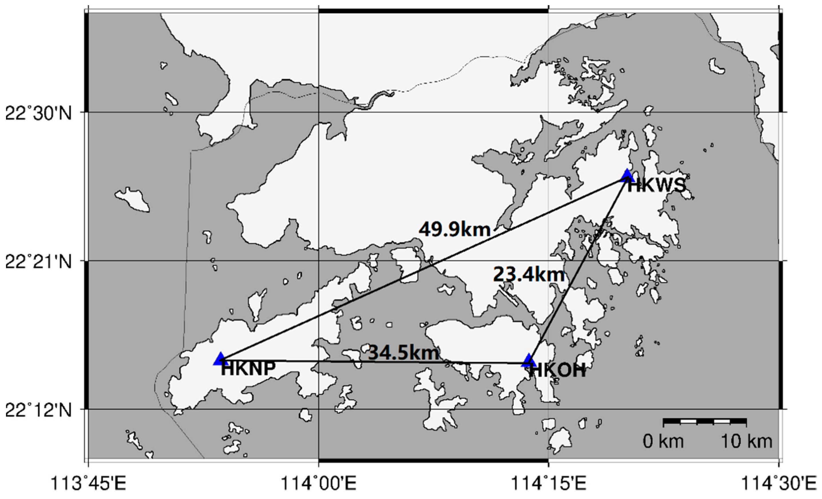
2. Materials and Methods

2.1. Fundamental Mathematical Models

The double-differenced (DD) code and carrier phase observations of linear-combined GNSS triple-frequency signals can be expressed as [26],

$$\{\begin{array}{c}∆\nabla P_{\left(i,j,k\right)}=∆\nabla \rho +∆\nabla {\delta }_{obt}+∆\nabla {\delta }_{trop}+{\beta }_{\left(i,j,k\right)}·∆\nabla \delta I_1\\ +{\mu }_{\left(i,j,k\right)}·∆\nabla {\epsilon }_{P_1} \\ ∆\nabla {\varphi }_{\left(i,j,k\right)}=∆\nabla \rho +\Delta \nabla {\delta }_{obt}+∆\nabla {\delta }_{trop}-{\beta }_{\left(i,j,k\right)}·∆\nabla \delta I_1\\ -{\lambda }_{\left(i,j,k\right)}·∆\nabla N_{\left(i,j,k\right)}+{\mu }_{\left(i,j,k\right)}·∆\nabla {\epsilon }_{{\varphi }_1}\end{array}$$

(1)

where the symbol $∆\nabla$ is the DD operator product,$P$ and $\varphi$ are the code and carrier phase observations in meters respectively, the subscript $\left(i,j,k\right)$ represents the combination coefficients of the individual frequencies used, $\rho$ represents the geometric distance from the satellite to the receiver, ${\delta }_{obt}$, ${\delta }_{trop}$ and $\delta I_1$ are the orbital bias, tropospheric delay and ionospheric delay of the first frequency, respectively, ${\beta }_{\left(i,j,k\right)}$ is the ionospheric scale factor (ISF) of the combination observations, ${\mu }_{\left(i,j,k\right)}$ is the noise factor of the combination observations, $\lambda$ and $N$ are the wavelength and integer ambiguity of the carrier phase, ${\epsilon }_{∆\nabla P}$ and ${\epsilon }_{∆\nabla \varphi }$ refer to the noise of code and carrier phase observations in meters. In the processing of reference stations, the station coordinates are a priori knowledge, thus $∆\nabla \rho$ can be directly real-time determined with the broadcast satellite coordinates.

The linear combinations of different signals can be obtained from the equations in Feng (2008) and the total noise level (TNL) for carrier phase combination observations in cycles are introduced [27]. TNL is considered as the main index in choosing the optimal-phase combinations, as a better choice for AR shall have a smaller TNL value.

$${\sigma }_{TNL}=\frac{\sqrt{{\left({\beta }_{\left(i,j,k\right)}·∆\nabla \delta I_1\right)}^2+∆\nabla {\delta }_{trop}{}^2+∆\nabla {\delta }_{obt}{}^2+{\left({\mu }_{\left(i,j,k\right)}·{\sigma }_{∆\nabla \varphi }\right)}^2}}{{\lambda }_{\left(i,j,k\right)}}$$

(2)

For the Galileo system, the three frequencies used are $f_1=f_{E1}$ (1575.42 MHz), $f_2=f_{E5b}$ (1207.14 MHz) and $f_3=f_{E5a}$ (1176.45 MHz), and the code and carrier phase observations in different frequencies are assumed to have common standard deviations (STD), respectively, i.e., ${\sigma }_{\Delta \nabla {\varphi }_i}={\sigma }_{\Delta \nabla \varphi }$ and ${\sigma }_{\Delta \nabla P_i}={\sigma }_{\Delta \nabla P}$ ($i=1,2,3$). We evaluated the TNL values from combinations of the coefficient $i,j,k$ in the range of $\left[-50,50\right]$, to identify the most useful combinations. The characteristics of some useful EWL and WL phase combinations are listed in

Table 1. Characteristics of some useful extra-wide-lane/wide-lane (EWL/WL) combinations for Galileo signals under three error budget scenarios.

Type	$\left(\mathit{i},\mathit{j},\mathit{k}\right)$	${\mathit{\lambda }}_{\left(\mathit{i},\mathit{j},\mathit{k}\right)}$	${\mathit{\beta }}_{\left(\mathit{i},\mathit{j},\mathit{k}\right)}$	${\mathit{\mu }}_{\left(\mathit{i},\mathit{j},\mathit{k}\right)}$	${\mathit{\sigma }}_{\mathit{T}\mathit{N}\mathit{L}}\left({\mathit{\sigma }}_{\Delta \nabla \mathit{\varphi }}=1 \mathbf{c}\mathbf{m}\right) \left(\mathit{c}\mathit{y}\mathit{c}\mathit{l}\mathit{e}\right)$
		(m)			${\mathit{\sigma }}_{\Delta \nabla \mathit{\delta }{\mathit{I}}_1}=20 \mathbf{c}\mathbf{m}$ ${\mathit{\sigma }}_{\Delta \nabla {\mathit{\delta }}_{\mathit{t}\mathit{r}}}=2.5 \mathbf{c}\mathbf{m}$ ${\mathit{\sigma }}_{\Delta \nabla {\mathit{\delta }}_{\mathit{o}\mathit{b}\mathit{t}}}=5 \mathbf{c}\mathbf{m}$	${\mathit{\sigma }}_{\Delta \nabla \mathit{\delta }{\mathit{I}}_1}=40 \mathbf{c}\mathbf{m}$ ${\mathit{\sigma }}_{\Delta \nabla {\mathit{\delta }}_{\mathit{t}\mathit{r}}}=5 \mathbf{c}\mathbf{m}$ ${\mathit{\sigma }}_{\Delta \nabla {\mathit{\delta }}_{\mathit{o}\mathit{b}\mathit{t}}}=5 \mathbf{c}\mathbf{m}$	${\mathit{\sigma }}_{\Delta \nabla \mathit{\delta }{\mathit{I}}_1}=100 \mathit{c}\mathit{m}$ ${\mathit{\sigma }}_{\Delta \nabla {\mathit{\delta }}_{\mathit{t}\mathit{r}}}=20 \mathit{c}\mathit{m}$ ${\mathit{\sigma }}_{\Delta \nabla {\mathit{\delta }}_{\mathit{o}\mathit{b}\mathit{t}}}=10 \mathit{c}\mathit{m}$
EWL	(0, 1, −1)	9.7684	−1.7477	54.9232	0.0669	0.0913	0.1889
	(1, −6, 5)	1.3955	−0.9889	44.0471	0.3483	0.4273	0.7922
	(1, −5, 4)	1.2211	−1.0838	31.8257	0.3187	0.4442	0.9430
	(1, −4, 3)	1.0854	−1.1576	22.3921	0.3012	0.4783	1.1056
WL	(1, −1, 0)	0.8140	−1.3051	5.3892	0.3345	0.6505	1.6279
	(1, 0, −1)	0.7514	−1.3391	4.9282	0.3700	0.7220	1.8080

, ordered by the combined wavelength.

In Table 1, three sets of representative error budgets are given for the scenarios of short, middle and long baselines [27], respectively. Rows 1–4 show the EWL combinations, whose wavelengths are longer than 1 m, while Rows 5–6 show the WL combinations, whose wavelengths are shorter than 1 m. According to the TNL index, ${\varphi }_{\left(0,1,-1\right)}$ and ${\varphi }_{\left(1,-6,5\right)}$ are selected as the optimal and the suboptimal EWL combinations for TCAR, respectively. Similarly, ${\varphi }_{\left(1,-1,0\right)}$ is chosen as the optimal WL combination for TCAR.

2.2. TCAR Methods

There are two kinds of TCAR methods, the GF TCAR method and the IF TCAR method, which are different in the treatment of observation biases. These two methods will be discussed in more details in the following sections. Considering that both methods could smooth the ambiguity over multiple epochs, the carrier phase observations are processed with cycle-slip detecting and repairing by TurboEdit algorithm [28]. In addition, the IF TCAR method was modified to combine multi-systems to improve the performance in terms of AR for original signals, and named as the combined IF (CIF) TCAR method.

2.2.1. Geometry-Free TCAR Method

Feng and Li (2008) introduced a GF TCAR method to resolve the ambiguities for reference stations using semi-simulated GPS triple-frequency data [23]. In this method, two EWL ambiguities are direct-determined as the first step, then two WL ambiguities are recovered; in the following, the ionospheric delay on L1 was obtained and refined by the Hatch smoothing process (Hatch 1982), and lastly, the original ambiguities on L1 could be determined [29].

In the Galileo signal processing, two GF EWL combinations, ${\varphi }_{\left(0,1,-1\right)}$ and ${\varphi }_{\left(1,-6,5\right)}$ in Table 1, are the optimal and suboptimal EWL combinations. Their ambiguities can be determined easily as

$$∆\nabla N_{\left(0,1,-1\right)}={\left[\left(∆\nabla P_{\left(0,1,1\right)}-∆\nabla {\varphi }_{\left(0,1,-1\right)}\right)/{\lambda }_{\left(0,1,-1\right)}\right]}_R$$

(3)

$$∆\nabla N_{\left(1,-6,5\right)}={\left[\left(∆\nabla P_{\left(0,1,1\right)}-∆\nabla {\varphi }_{\left(1,-6,5\right)}\right)/{\lambda }_{\left(1,-6,5\right)}\right]}_R$$

(4)

where ${[*]}_R$ is the rounding operator product, Equation (4) is the Hatch–Melbourne–Wübbena (HMW) combination with E5b and E5a, which has a long wavelength of 9.7684 m [29,30,31]. The result is free from most errors, and only the measurement noise of code and phase observations have an adverse effect on this combination. The suboptimal combination, Equation (4), is influenced by both the measurement noise and the ionospheric delay residual.

After fixing the ambiguities on $∆\nabla N_{\left(0,1,-1\right)}$ and $∆\nabla N_{\left(1,-6,5\right)}$, two WL ambiguities can be determined directly as

$$∆\nabla N_{\left(1,-1,0\right)}=∆\nabla N_{\left(1,-6,5\right)}+5∆\nabla N_{\left(0,1,-1\right)}$$

(5)

$$∆\nabla N_{\left(1,0,-1\right)}=∆\nabla N_{\left(1,-6,5\right)}+6∆\nabla N_{\left(0,1,-1\right)}$$

(6)

In the following, the ionospheric delay on E1 can be calculated from the two fixed WL ambiguities as

$$∆\nabla I_1=\frac{f_2{f}_3\left[{\lambda }_{\left(1,-1,0\right)}∆\nabla N_{\left(1-1,0\right)}+∆\nabla {\varphi }_{\left(1-1,0\right)}-{\lambda }_{\left(1,0,-1\right)}∆\nabla N_{\left(1,0,-1\right)}-∆\nabla {\varphi }_{\left(1,0,-1\right)}\right]}{f_1\left(f_2-f_3\right)}$$

(7)

In this processing, the phase noise is amplified about 129.86 times in $∆\nabla I_1$, thus it is necessary to refine the ionospheric delay by the Hatch smoothing process with the ionospheric delay $∆\nabla I_1^{\prime }$, which is derived from the original phase observations with unknown ambiguities over multiple epochs [32],

$$∆\nabla I_1^{\prime }=\frac{f_2^2}{f_1^2-f_2^2}\left[∆\nabla {\varphi }_{\left(1,0,0\right)}-∆\nabla {\varphi }_{\left(0,1,0\right)}\right]$$

(8)

$$∆\nabla {\overline{I}}_1\left(k\right)=\frac{1}{k}∆\nabla I_1\left(k\right)+\frac{k-1}{k}\left[∆\nabla {\overline{I}}_1\left(k-1\right)+∆\nabla I_1^{\prime }\left(k\right)-∆\nabla I_1^{\prime }\left(k-1\right)\right]$$

(9)

where $∆\nabla {\overline{I}}_1\left(k\right)$ represents the refined ionospheric delay on E1 at the $k^{th}$ epoch.

At the last step, the ambiguity of the first frequency $∆\nabla N_1$ can be determined by smoothing over $k$ epochs,

$$∆\nabla N_1={\left[\frac{1}{k}{{\displaystyle \sum }}_{i=1}^k\frac{{\lambda }_{\left(1,-1,0\right)}∆\nabla N_{\left(1-1,0\right)}+∆\nabla {\varphi }_{\left(1-1,0\right)}-∆\nabla {\varphi }_1+\Delta \nabla {\overline{I}}_{\left(1-1,0\right)}\left(i\right)-∆\nabla {\overline{I}}_1\left(i\right)}{{\lambda }_1}\right]}_R$$

(10)

All the steps of the GF TCAR method are free from geometry-based errors, and the ambiguity $∆\nabla N_1$ is influenced only by the amplified noise and the refined ionospheric delay.

2.2.2. Ionospheric-Free TCAR Method

The IF TCAR method was proposed by Tang et al. (2018) for BDS reference station TCAR. This method starts from fixing the optimal EWL ambiguity $\Delta \nabla N_{\left(0,1,-1\right)}$ in Equation (3) [25]. It is the same procedure as in GF TCAR.

After $∆\nabla N_{\left(0,1,-1\right)}$ is fixed, the optimal WL ambiguity $∆\nabla N_{\left(1,-1,0\right)}$ could be fixed in the following. Since the positions of reference stations are a priori knowledge, $∆\nabla \rho$ can be determined directly, then the ambiguities of two carrier-phase IF combinations can be obtained as

$$\Delta \nabla {\widehat{N}}_{LC12}=\left(∆\nabla \rho +\Delta \nabla {\delta }_{obt}+∆\nabla {\delta }_{trop}\right)/{\lambda }_{LC12}-∆\nabla {\phi }_{LC12}$$

(11)

$$\Delta \nabla {\widehat{N}}_{LC13}=\left(∆\nabla \rho +∆\nabla {\delta }_{obt}+∆\nabla {\delta }_{trop}\right)/{\lambda }_{LC13}-∆\nabla {\phi }_{LC13}$$

(12)

where the subscript $LC12$ and $LC13$ represent the coefficient combinations $\left(1,-f_2/f_1,0\right)$ and $\left(1,0,-f_3/f_1\right)$, respectively. In the actual data processing, $∆\nabla {\delta }_{obt}$ can be neglected for the baseline under 100 km, and the dry component of the tropospheric delay $∆\nabla {\delta }_{tr}$ can be estimated from the Hopfield model [33] and the Niell mapping function (NMF) [34].

After fixing $∆\nabla N_{\left(0,1,-1\right)}$, $\Delta \nabla {\widehat{N}}_{LC12}$ and $\Delta \nabla {\widehat{N}}_{LC13}$, the WL ambiguity $\Delta \nabla {\widehat{N}}_{\left(1,-1,0\right)}$ can be computed as

$$\Delta \nabla {\widehat{N}}_{\left(1,-1,0\right)}=K_1\Delta \nabla {\widehat{N}}_{LC12}+K_2\Delta \nabla {\widehat{N}}_{LC13}+K_3\Delta \nabla N_{\left(0,1,-1\right)}$$

(13)

where $K_1$, $K_2$ and $K_3$ are given as

$$\{\begin{array}{c}{K}_1=\left({\lambda }_2{\lambda }_3-{\lambda }_2{\lambda }_1\right)/\left({\lambda }_1{\lambda }_3-{\lambda }_2{\lambda }_1\right)\\ K_2=\left({\lambda }_1{\lambda }_3-{\lambda }_2{\lambda }_3\right)/\left({\lambda }_1{\lambda }_3-{\lambda }_2{\lambda }_1\right)\\ K_3=\left({\lambda }_2{\lambda }_1-{\lambda }_1{\lambda }_1\right)/\left({\lambda }_1{\lambda }_3-{\lambda }_2{\lambda }_1\right)\end{array}$$

(14)

Substituting Equations (11) and (12) to Equation (13)

$$\begin{gathered} \Delta \nabla {\widehat{N}}_{\left(1,-1,0\right)}=\frac{K_1·\left(∆\nabla \rho -∆\nabla {\delta }_{trop}-∆\nabla {\delta }_{obt}-∆\nabla {\varphi }_{LC12}\right)}{{\lambda }_{LC12}} \\ +\frac{K_2·\left(∆\nabla \rho -∆\nabla {\delta }_{trop}-∆\nabla {\delta }_{obt}-∆\nabla {\varphi }_{LC13}\right)}{{\lambda }_{LC13}}+K_3·\Delta \nabla N_{\left(0,1,-1\right)} \end{gathered}$$

(15)

As Equation (15) shows, the tropospheric delay, the orbital bias and the amplified phase observation noise may prevent the AR fixing for the WL combination. In the Galileo system, the combined observation noise is the major noise factor and amplifies the phase noise more than 50 times. Thus, a smoothing processing is necessary in fixing the WL combination ambiguity

$$\Delta \nabla N_{\left(1,-1,0\right)}={\left[\frac{1}{k}·{\displaystyle \sum }_1^k\Delta \nabla {\widehat{N}}_{\left(1,-1,0\right)}\right]}_R$$

(16)

where the coefficient $k$ represents the $k^{th}$ epoch, the smoothing process averages the float ambiguities of all the former results.

In Equation (11), $\Delta \nabla {\widehat{N}}_{LC12}$ is back-calculated from $∆\nabla \rho$, although the orbital bias and the tropospheric delay wet component still exist, they are neglectable on the AR solving for the WL combination. However, the precision of this IF combination ambiguities cannot be sufficient for the E1 AR. Thus, a Kalman Filter (KF) is required to estimate the IF combination ambiguities and the wet component of tropospheric delay

$$\left[\begin{array}{c}{l}_{PC12}\\ l_{LC12}\\ l_{LC13}\end{array}\right]=\left[\begin{array}{cccc}{M}_1& -M_2& 0& 0\\ M_1& -M_2& {\lambda }_{LC12}·I& 0\\ M_1& -M_2& 0& {\lambda }_{LC13}·I\end{array}\right]\left[\begin{array}{c}dZT{D}_{w1}\\ dZT{D}_{w2}\\ \begin{array}{c}\Delta \nabla {\tilde{N}}_{LC12}\\ ∆\nabla {\tilde{N}}_{LC13}\end{array}\end{array}\right]+\left[\begin{array}{c}{v}_{PC12}\\ v_{LC12}\\ v_{LC13}\end{array}\right]$$

(17)

where $l$ represents the combined observation minus the computed distance after bias corrections, the subscript $PC12$ means the code IF combination using P1 and P2. $M_1$ and $M_2$ are the mapping coefficients of zenith tropospheric delay (ZTD) for each station using the NMF model, and $I$ is the identity matrix. $dZT{D}_{w1}$ and $dZT{D}_{w2}$ are the ZTD wet components of two reference stations. $v$ is the observation residual.

Since $\Delta \nabla N_{\left(1,-1,0\right)}$ is obtained from Equation (16) and $∆\nabla {\tilde{N}}_{LC12}$ can be estimated from KF with a higher precision, the E1 ambiguity can be solved as

$$\Delta \nabla N_1={\left[\left(f_1·∆\nabla {\tilde{N}}_{LC12}-f_2·∆\nabla N_{\left(1,-1,0\right)}\right)/\left(f_1-f_2\right)\right]}_R$$

(18)

2.2.3. Combined Ionospheric-Free TCAR Method

In order to take advantage of multi-system triple-frequency data, the IF TCAR method could be modified in the step of original signal AR as the CIF TCAR method. Specifically speaking, Equation (17) is replaced by Equation (19)

$$\left[\begin{array}{c}{l}_G\\ l_E\end{array}\right]=\left[\begin{array}{cccc}{M}_1& -M_2& {\lambda }_G& 0\\ M_1& -M_2& 0& {\lambda }_E\end{array}\right]\left[\begin{array}{c}dZT{D}_{w1}\\ dZT{D}_{w2}\\ \Delta \nabla {\tilde{N}}_G\\ ∆\nabla {\tilde{N}}_E\end{array}\right]+\left[\begin{array}{c}{v}_G\\ v_E\end{array}\right]$$

(19)

where the subscript G, E represent different systems, $l$, $\lambda$, $∆\nabla N$ and $v$ include three different observation types (PC12, LC12, LC13). As in different systems, different reference satellites are selected to conduct the DD operation within each system, thus the ISBs (Inter-System Bias) can be ignored.

3. Results

To evaluate the Galileo TCAR performance, three experiments were conducted with the common data collected by Leica GR50 receivers from the Hong Kong Continuously Operating Reference Stations (CORS) network on DOY 001, 2018, the sampling interval was one second, three reference stations named HKNP, HKOH and HKWS were chosen to form a closure ring of the network; accordingly, their baseline lengths were 23.4 km, 34.5 km and 49.9 km, respectively, and the locations were illustrated in Figure 1. Position and Navigation Data Analyst (PANDA) software originally developed by Wuhan University was modified to verify the performance of the Galileo TCAR [35]. The first experiment was conducted in the Galileo system to illustrate the Galileo TCAR performance by the IF TCAR method in comparison of the GF TCAR method.

3.1. Galileo Data by GF and IF TCAR Methods

In the Galileo system, three frequencies (E1, E5b, and E5a) were used to resolve the ambiguities. With mask angle 10°, the number of observed Galileo DD satellite pairs in three baselines is shown in Figure 2.

The selected stations were close enough to consider the synchronous observed Galileo satellites, as shown in Figure 2. Due to the limited number of observable Galileo satellites in the Hong Kong area, the number of Galileo DD satellite pairs was no more than 6 on this day. The IOV satellites were ignored, because they will not be operational anymore and three FOC satellite pairs (E09–E04, E05–E04, and E24–E04) were selected to show the TCAR performance. The true value of the ambiguity was obtained from precise post-processing and validated by the closure ring of the triangle network [25].

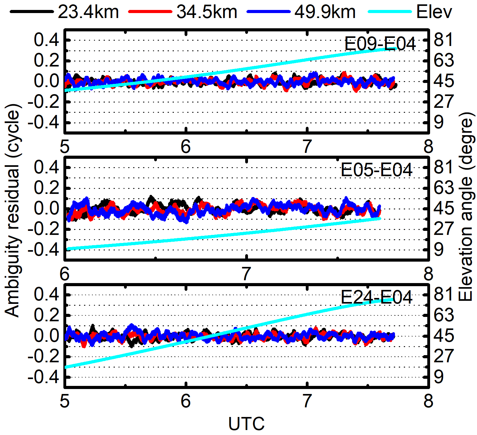
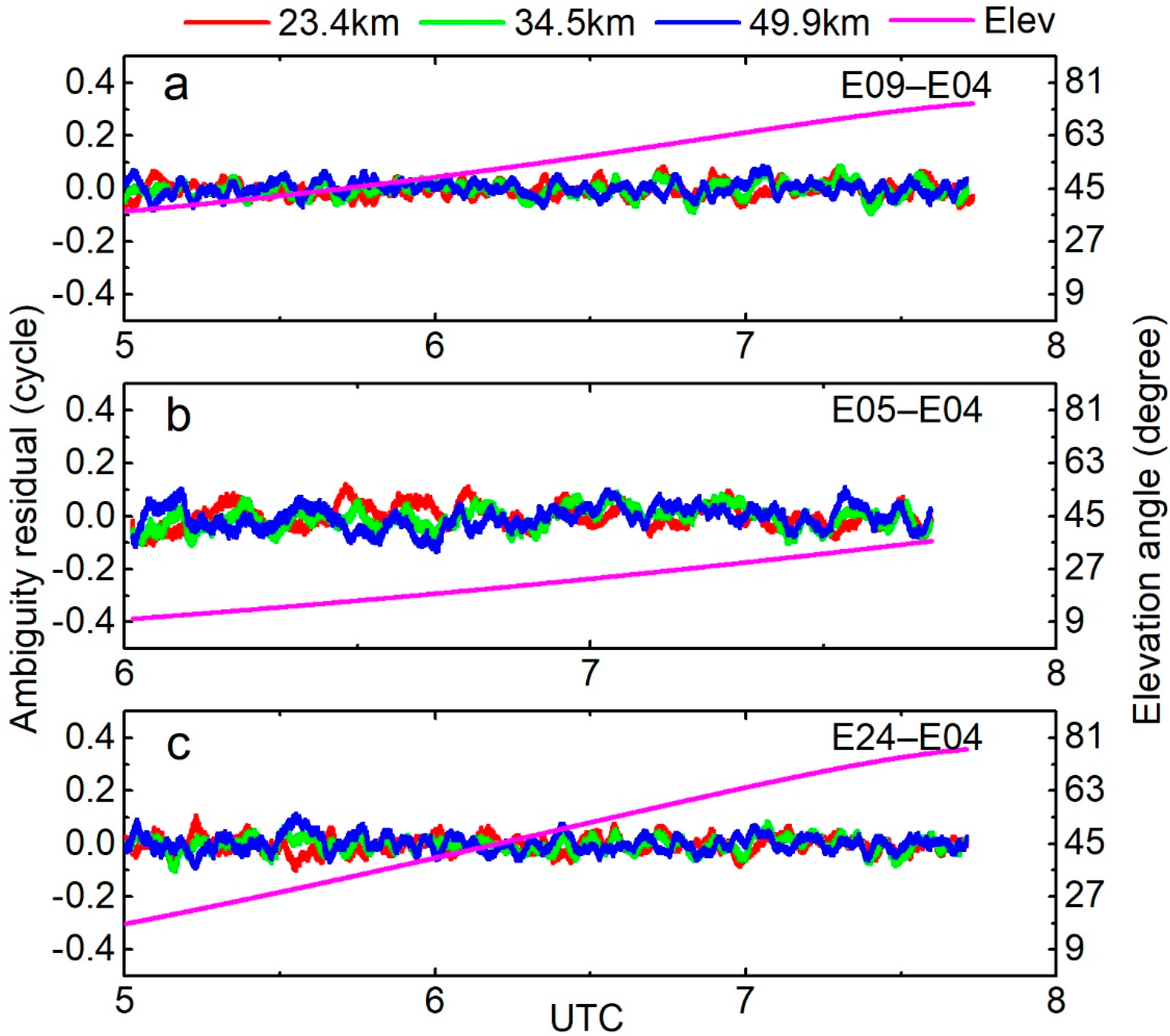
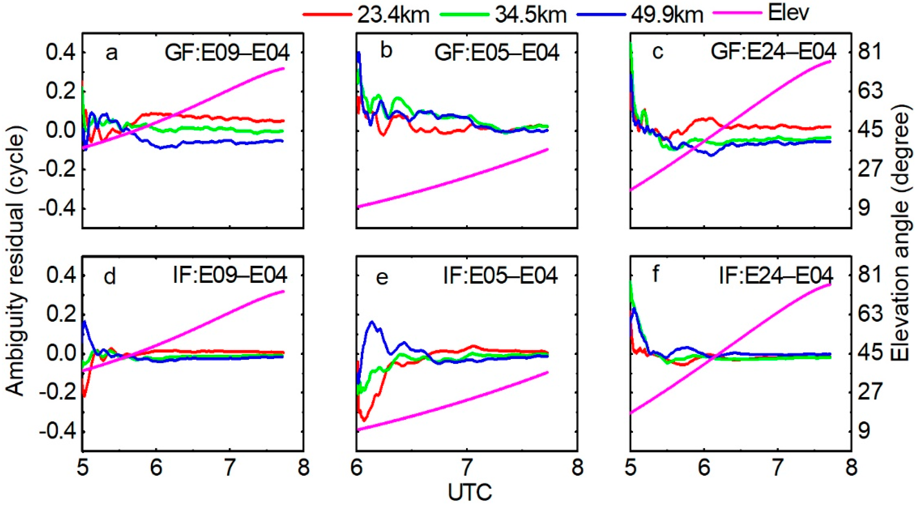
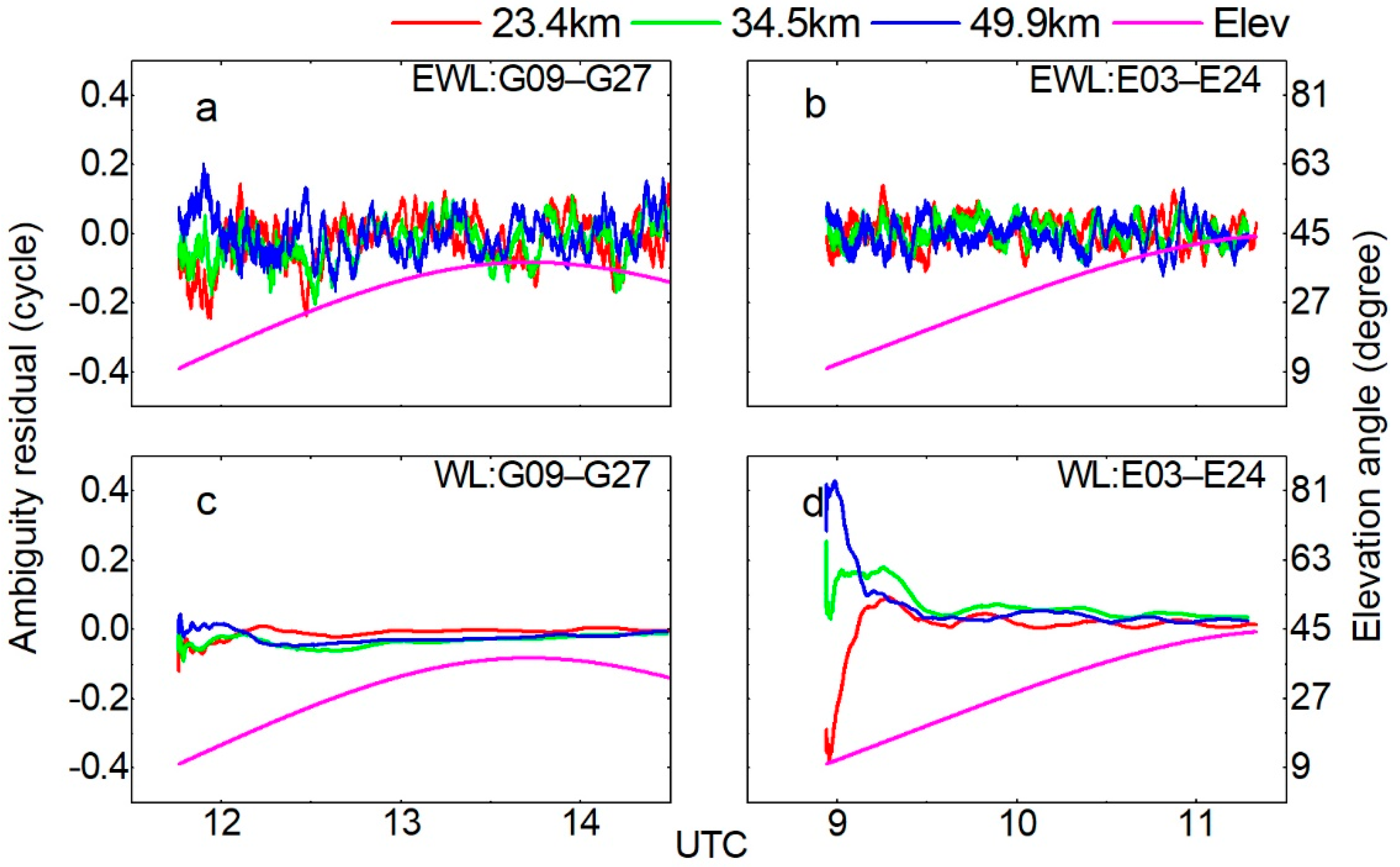
3.1.1. AR for the Optimal EWL Combination

In both TCAR methods, $∆\nabla N_{\left(0,1,-1\right)}$ is resolved by the HMW combination with E5b and E5a signals with a long wavelength about 9.7684 m, the HMW combination cancels the ionospheric delay, the tropospheric delay and the orbital bias, and only the measurement noise for code and phase observations could prevent AR. Figure 3 demonstrates the ambiguity residual of $∆\nabla N_{\left(0,1,-1\right)}$ with the Galileo data and the satellite elevation angle in selected baselines, the ambiguity residual is defined as the difference between the resolved ambiguity before rounding and the true value. It can be seen that the ambiguity residual is fluctuated within $\pm 0.1$ cycles, the rounding operation can fix $∆\nabla N_{\left(0,1,-1\right)}$ correctly and reliably in a single epoch.

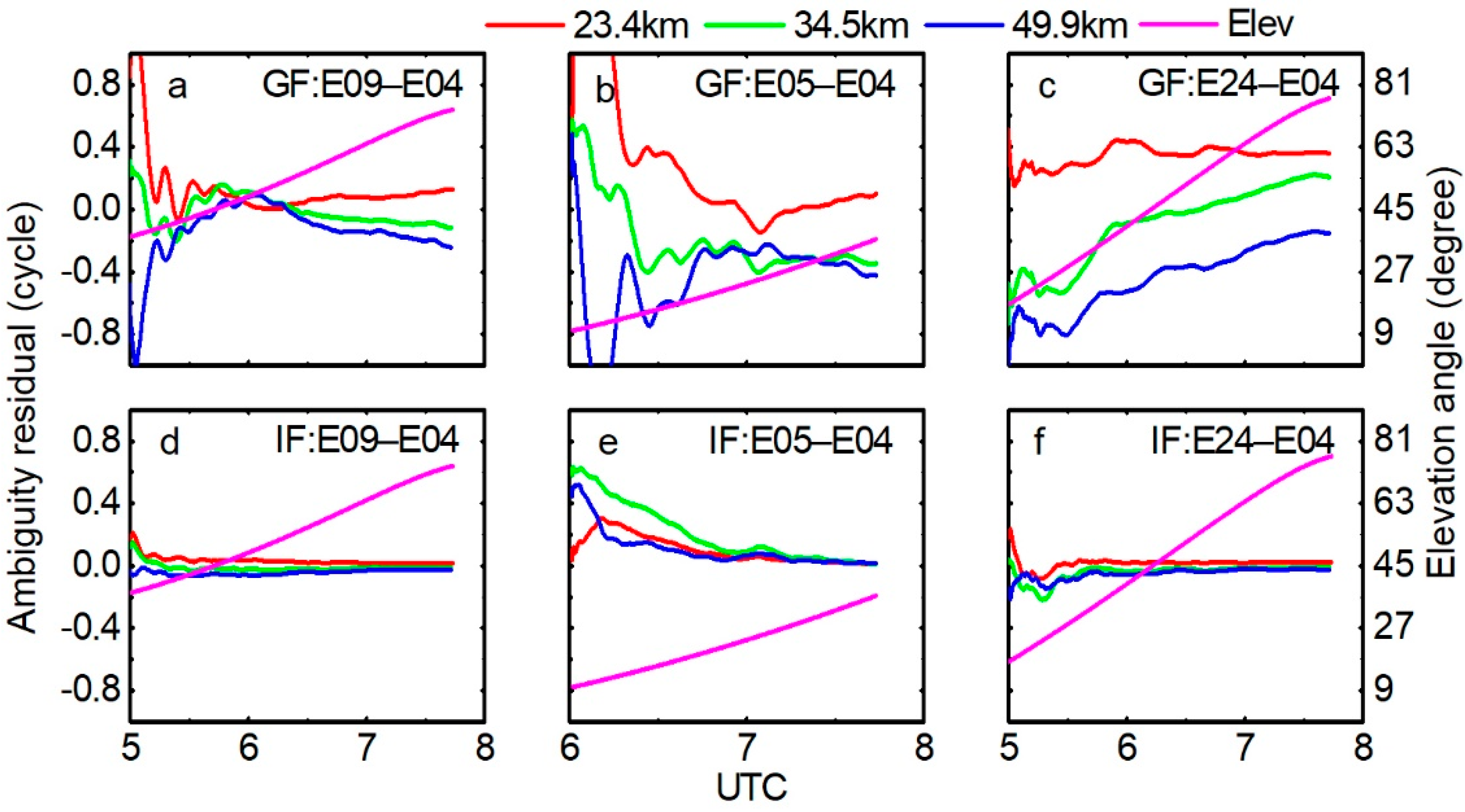
3.1.2. AR for the Optimal WL Combination

After $∆\nabla N_{\left(0,1,-1\right)}$ is fixed correctly, $∆\nabla N_{\left(1,-1,0\right)}$ could be solved. In the GF TCAR method, Equation (5) has shown that $∆\nabla N_{\left(1,-1,0\right)}$ is dominated by $∆\nabla N_{\left(1,-6,5\right)}$ obtained from Equation (4). The single-epoch mode for $∆\nabla N_{\left(1,-6,5\right)}$ AR is unreliable and we have to smooth the float ambiguities in Equation (16) with previous observed epochs; the ambiguity residual of $∆\nabla N_{\left(0,1,-1\right)}$ and the satellite elevation angle by two TCAR methods after smoothing is shown in Figure 4. Meanwhile,

Table 2. The mean RMS of the Galileo WL ambiguity residuals and the convergence time.

Method	E09–E04		E05–E04		E24–E04
	RMS (cycle)	T (s)	RMS (cycle)	T (s)	RMS (cycle)	T (s)
GF TCAR	0.0497	57.3	0.0733	568.7	0.0610	1308.0
IF TCAR	0.0298	175.3	0.0688	562.3	0.0456	468.1

shows the mean Root Mean Square (RMS) of the three groups of WL ambiguity residuals and the time to converge to the true value ±0.10 cycle.

In Figure 4, we could find that the results by the IF TCAR method are more stable and precise than the results by the GF TCAR method. The reason is that the IF TCAR method cancels most of the ionospheric delay and does not use the code measurement to calculate the WL combination ambiguity, which could take more time to smooth the noise. It should be noted from Table 2 that the convergence time of the E09–E04 for the GF TCAR method is out of exception. The main reason is that the double-differenced satellites in this group have a higher elevation angle and lower noise. So, the advantage of the IF TCAR method without using code observations is not obvious. However, the final convergence value of GF TCAR does not converge to near zero, and the RMS value is less than 0.05 cycle, which is still not as good as the result of IF TCAR. On the whole, the IF TCAR method with respect to GF TCAR improves the accuracy by 21.6% and the convergence speed by 37.6%, respectively. The IF TCAR method improves the WL AR for $∆\nabla N_{\left(1,-1,0\right)}$ clearly.

3.1.3. AR for the E1 Signal

$∆\nabla N_{\left(0,1,-1\right)}$ and $∆\nabla N_{\left(1,-1,0\right)}$ can be determined correctly and reliably in both TCAR methods, the major challenge to Galileo TCAR is to fix the E1 ambiguity properly. The GF TCAR method calculates $∆\nabla \delta I_1$ by two fixed WL combination ambiguities in Equation (7) and refines the result over several minutes by Hatch smoothing in Equations (8) and (9). It can be found that $∆\nabla N_{\left(1,-1,0\right)}$ and $∆\nabla N_{\left(1,0,-1\right)}$ can be fixed correctly, then, the ionospheric delay obtained from Equation (7) is unbiased, only the phase noise is amplified by 129.86 times. Here, we smooth the ionospheric delay over 120 s in Equation (9), which implies that the ionosphere is relatively stable within 2 min [27]. Regarding the IF TCAR method, the ambiguity $\Delta \nabla {\widehat{N}}_{LC12}$ obtained by Equation (11) is not good enough for the E1 AR, due to the tropospheric delay wet component and the orbital bias left in $\Delta \nabla {\widehat{N}}_{LC12}$; the IF TCAR method could estimate a more precise $\Delta \nabla {\tilde{N}}_{LC12}$ by KF to determine the E1 ambiguity. Figure 5 shows the E1 ambiguity residual and the corresponding satellite elevation angle by two TCAR methods. Meanwhile, the mean RMS and the time to converge to the true value ±0.20 cycle of the two TCAR methods are shown in

Table 3. The mean RMS of the E1 ambiguity residuals and the convergence time.

Method	E09–E04		E05–E04		E24–E04
	RMS (cycle)	T (s)	RMS (cycle)	T (s)	RMS (cycle)	T (s)
GF TCAR	0.1938	933.3	0.4693	+∞	0.3683
IF TCAR	0.0389	34.0	0.1881	1456.1	0.0541	718.3

. Since the E05–E04 and E24–E04 in the GF TCAR method finally failed to converge to ±0.2 cycle, the corresponding convergence time is +∞.

In Figure 5, we could clearly find that both methods could fix the E1 ambiguity of the FOC satellite pairs correctly with a smooth processing, but the IF TCAR method is more reliable than the GF TCAR method. Moreover, the E1 accuracy of the IF TCAR method is improved by 72.7% compared with the GF TCAR method.

Comparing the performance of two TCAR methods in the Galileo system, we could find that the Galileo system is able to realize TCAR correctly using either TCAR method, while IF TCAR has a better performance than GF TCAR in terms of WL AR and E1 AR.

Compared with Galileo TCAR performance, another experiment of GPS TCAR performance has been carried out and will be given in the following section.

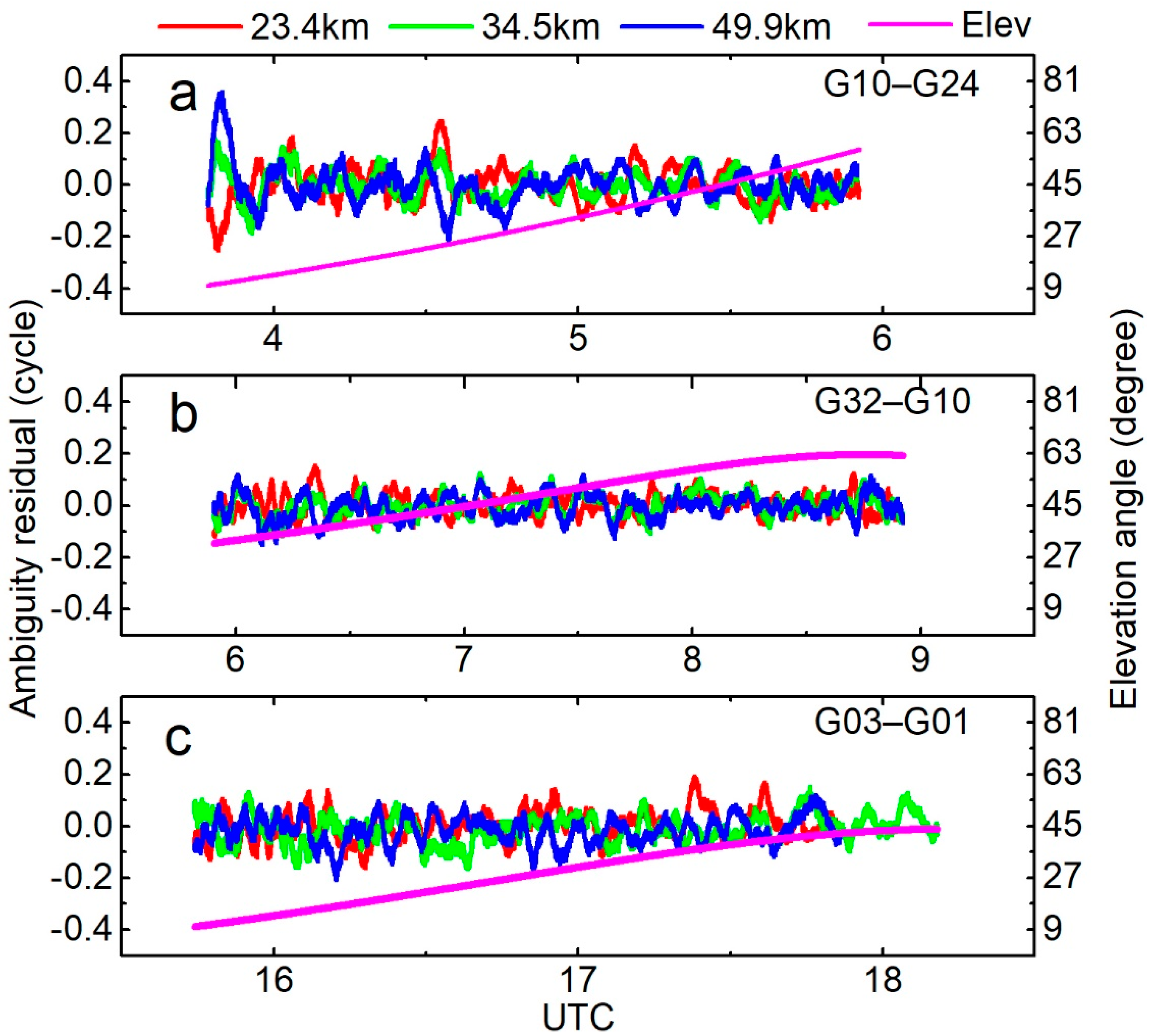
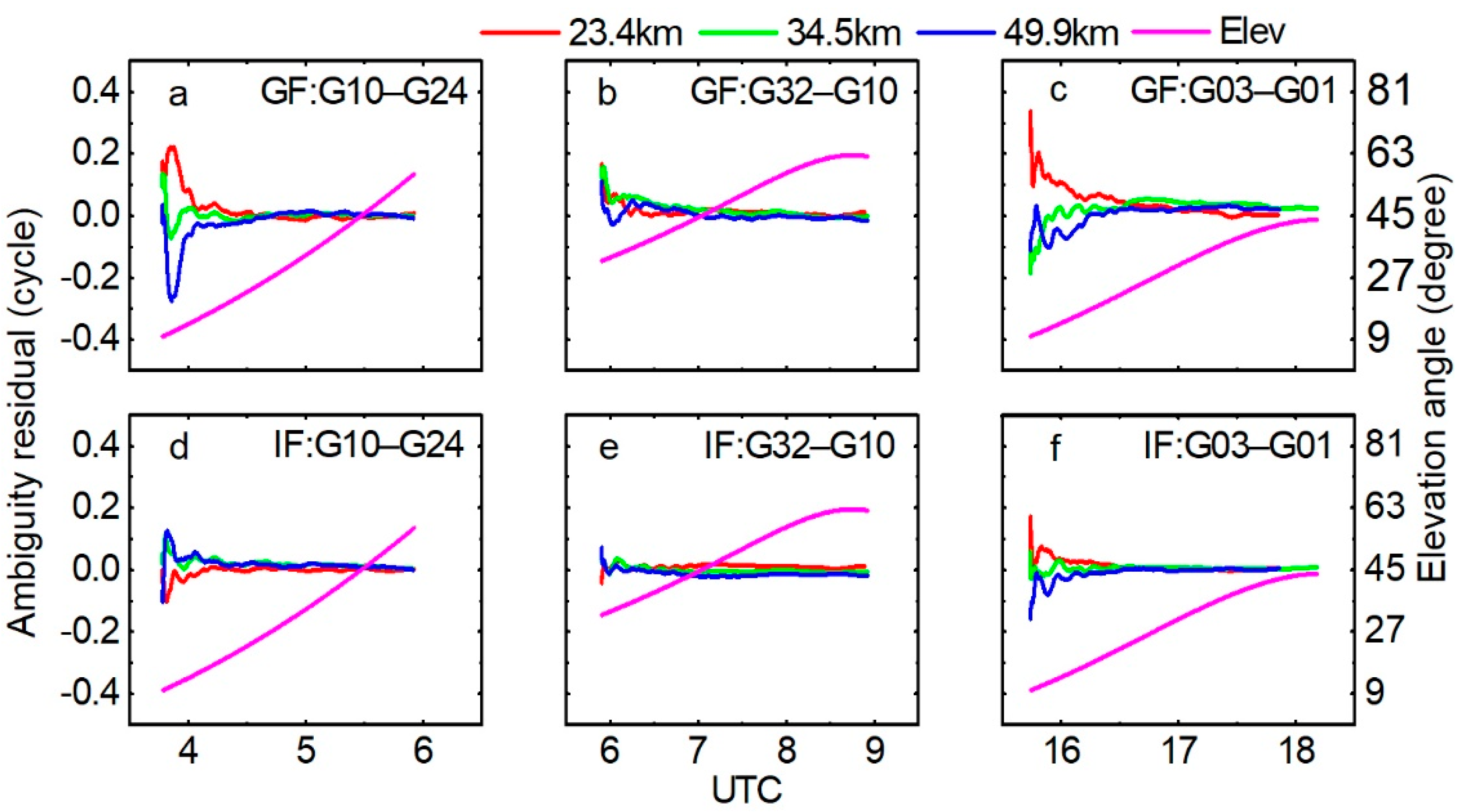
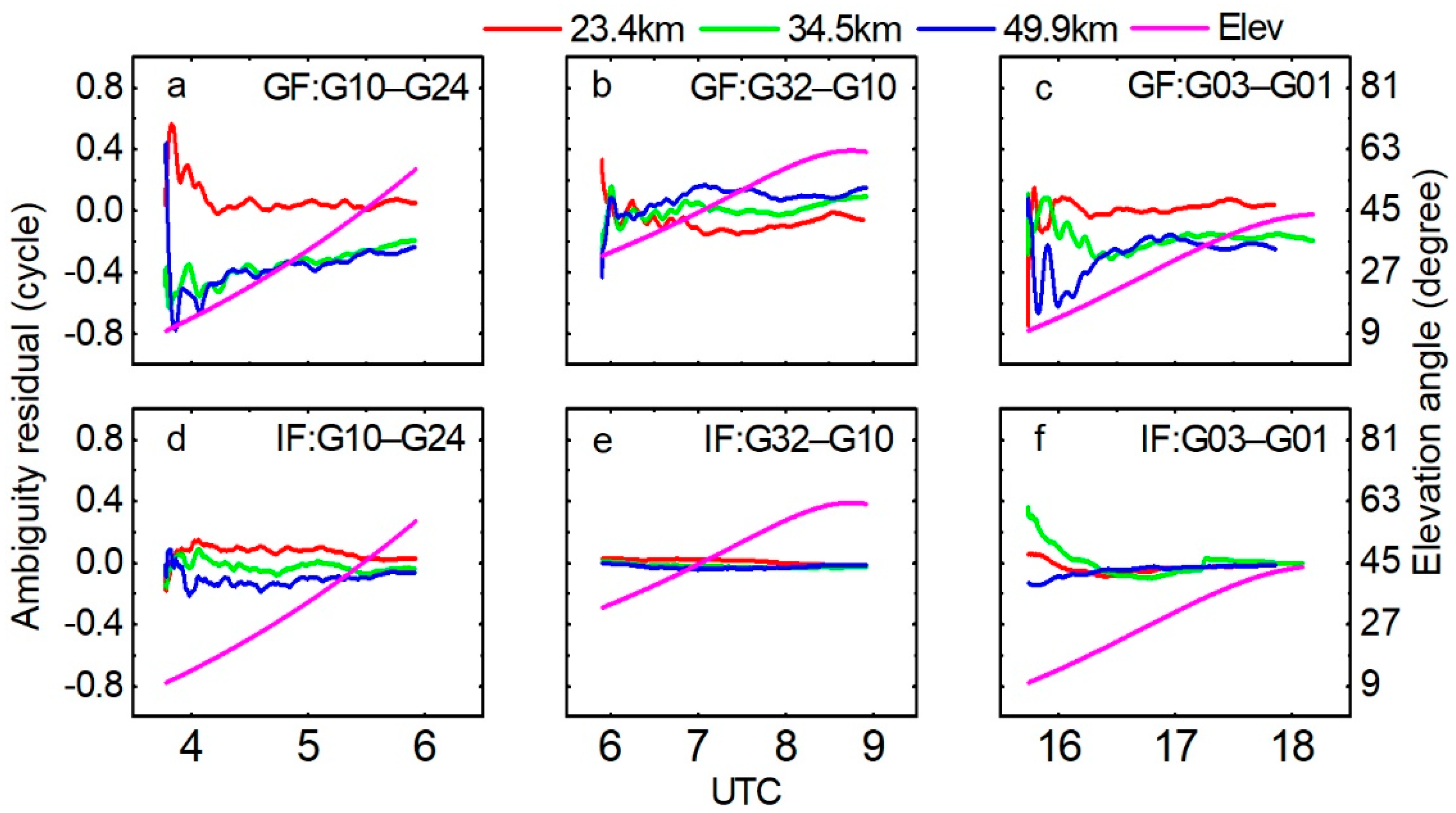
3.2. GPS Data by GF and IF TCAR Methods

For comparison, we also provided GPS TCAR performance by the same methods. There are 12 GPS satellites transmitting the third frequency L5 signal, and the number of visible GPS DD satellite pairs in selected baselines on DOY 001, 2018 is plotted in Figure 6, the DD satellite number of GPS is less than that of Galileo in the Hong Kong area.

The same strategy was adopted in GPS TCAR, and three arbitrary DD satellite pairs (G10–G24, G32–G10, G03–G01) were chosen to illustrate the performance of GPS triple-frequency data by two TCAR methods. The residual of $∆\nabla N_{\left(0,1,-1\right)}$ and the satellite elevation angle are shown in Figure 7; the result of GPS is similar to that of Galileo in Figure 3; both systems could use the HMW combination to determine $∆\nabla N_{\left(0,1,-1\right)}$ reliably in a single epoch.

Figure 8 shows the residual of $∆\nabla N_{\left(1,-1,0\right)}$ by using GF TCAR and IF TCAR, respectively. For the GPS data, the suboptimal EWL combination is still ${\varphi }_{\left(1,-6,5\right) }$ [27]. The optimal WL ambiguity $∆\nabla N_{\left(1,-1,0\right)}$ is determined by $∆\nabla N_{\left(1,-6,5\right)}$ in the GF TCAR method. Both methods could also determine $∆\nabla N_{\left(1,-1,0\right)}$ ambiguity correctly and reliably and the result of GPS are similar to that of Galileo in the GF TCAR method, as shown in Figure 4. Meanwhile, the mean RMS and the time to converge to the true value ±0.10 cycle of the three group WL ambiguity residuals are shown in

Table 4. The mean RMS and the convergence time of the GPS WL ambiguity.

Method	G10–G24		G32–G10		G03–G01
	RMS (cycle)	T (s)	RMS (cycle)	T (s)	RMS (cycle)	T (s)
GF TCAR	0.0442	366.3	0.0252	70.0	0.0464	147.0
IF TCAR	0.0233	4.0	0.0122	1.0	0.0180	45.3

. Compared with the GF TCAR method, it can be seen from Table 4 that the GPS WL accuracy and the convergence time of the IF TCAR method are improved by 53.7% and 91.3%, respectively.

Figure 9 shows the GPS L1 ambiguity residual by using two TCAR methods; both methods could fix the ambiguity correctly. Again, the IF TCAR method outperforms GF TCAR in terms of the residual level and convergence time. The mean RMS of the three group L1 ambiguity residuals and the time to converge to the true value ±0.20 cycle are shown in

Table 5. The mean RMS and the convergence time of the GPS L1 ambiguity.

Method	G10–G24		G32–G10		G03–G01
	RMS (cycle)	T (s)	RMS (cycle)	T (s)	RMS (cycle)	T (s)
GF TCAR	0.2973	5136.7	0.0847	80.0	0.1861	2483.7
IF TCAR	0.0785	252.3	0.0236	1.0	0.0629	200.5

. From Table 5, it can be found that the L1 accuracy and the convergence time of the IF TCAR method are improved by 70.9% and 94.1%, respectively.

The last experiment was conducted whereby the CIF TCAR method was applied in a selected dataset of combined GPS and Galileo to resolve the ambiguity of the original signals with the comparison of GPS-only and Galileo-only IF TCAR.

3.3. GPS and Galileo Data by CIF TCAR Method

The Hong Kong CORS network provided the triple-frequency signals of GPS and Galileo at the same time; we could use GPS and Galileo combination data on DOY 001, 2018 to conduct CIF TCAR, and the number of DD satellites which could transmit triple-frequency signals is shown in Figure 10.

The DD satellite pairs G09–G27 in the GPS system and E03–E24 in the Galileo system were chosen to illustrate the TCAR performance; the strategy of AR for the EWL and WL combinations is identical to the IF TCAR method with the residuals calculated in the independent system and the corresponding elevation angles, as shown in Figure 11. The ambiguities of EWL and WL combinations could be fixed easily in both systems.

Table 6. The mean RMS and the convergence time of the CIF TCAR method.

System	G09–G27		E03–E24
	RMS (cycle)	T (s)	RMS (cycle)	T (s)
GPS	0.0983	230.3
Galileo			0.2509	2039.3
GPS + Galileo	0.0864	42.3	0.1729	1785.7

shows the mean RMS and the time to converge to the true value ±0.10 cycle.

We focused on the AR for the original signals, Figure 12 plotted the ambiguity residuals of original signal L1 and E1 in the independent system and in the combined system. Both systems can also fix the ambiguity reliably; however, the CIF TCAR method accelerated the convergence of original signals in both systems clearly, for the reason of more available satellites, which means that the GPS triple-frequency data could be used to improve Galileo TCAR performance. Table 6 shows the mean RMS and the time to converge to the true the value ±0.20 cycle for GPS and Galileo combination. From Table 6, it can be found that the GPS and Galileo combined IF TCAR method can effectively improve the accuracy of the ambiguity resolution, and at the same time accelerate the convergence of the L1 or E1 ambiguity. In generally, the combined system has an average increase of 25.7% accuracy and 47.1% convergence time compared to the single GPS or Galileo.

4. Discussion

Since the Galileo system is a developing and valuable navigation system and the responding research is under development, we focused on analyzing the triple-frequency ambiguity resolution performance between reference stations in the Galileo system. Meanwhile, the work we analyzed and assessed here was the first step of the NRTK procedure, which was followed by the generation of atmosphere corrections as the second step and the solving of the positioning domain as the third step. The improvement was only on the float ambiguity between reference stations, improving both the precision and convergence speed. Further, the results of this paper are expected to provide useful references for future research of Galileo triple-frequency ambiguity resolution. Meanwhile, the effectiveness and reliability of ambiguity resolution between reference stations is the key for NRTK to provide reliable navigation and position services. For the ambiguity resolution of reference stations in NRTK, the coordinates of reference stations have been precisely known, and we do not need to resolve the ambiguity of all satellites. The TCAR method focuses on resolving the ambiguity based on a single double-differenced satellite pair and will be more efficient and appropriate. Therefore, the research and analysis of the TCAR method is of great significance to GAL NRTK. The number of satellites of the Galileo in the Hong Kong area is limited, and its three-frequency ambiguity has a large difference between the two TCAR algorithms. The ambiguity residuals solved by the GF TCAR method are difficult to converge to the true E1 or L1 value, while the IF TCAR method could still resolve its ambiguity resolution very reliably. The accuracy and the convergence time of the ambiguity resolution could be effectively improved by the GPS and Galileo combined IF TCAR method.

However, the test data are not large enough. So, further experiments need to continue with large data considering the state of the ionosphere, included the geographical latitude, season and time of day, as well as solar activity. With the opening of the global service of BDS3, in the future, we could study and analyze the TCAR method with BDS. The study Galileo and multi-system TCAR is expected to further improve the ambiguity resolution between reference stations, so as to provide GNSS users with more effective NRTK services.

5. Conclusions

In this paper, we discussed the Galileo triple-frequency optimal combinations for TCAR using E1, E5a, and E5b signals. Then, we introduced two TCAR methods for the Galileo system, i.e., the GF TCAR method and the IF TCAR method. The GF TCAR method is free from geometry-based errors, which include the tropospheric delay and the orbital bias, while the IF TCAR method could cancel most of the ionospheric delay. Then, the IF TCAR method is modified to resolve multi-system triple-frequency ambiguity. Finally, three experiments were conducted in the Hong Kong area; the first one was to evaluate GF TCAR and IF TCAR AR performance in the current stage Galileo service, the second test was to compare the Galileo with GPS in terms of TCAR performance, the last experiment was to further analyse the advantage of a combined system in the TCAR performance.

In the Galileo system, all methods choose a HMW combination with E5b and E5a to determine the EWL combination ambiguity correctly and reliably. For the WL AR, the GF and IF TCAR methods could also fix the ambiguity correctly after a smoothing processing, while the IF TCAR method could converge to the true ambiguity in a shorter time and also could be more reliable. Although both methods take different strategies to determine the WL ambiguities, they both could fix the WL ambiguity correctly. In terms of fixing the E1 ambiguity, these two methods have different performances. The GF TCAR method calculates the ionospheric delay and refines the result over 120 s, in which period the ionospheric delay is assumed to be stable. At the last step, the E1 ambiguity is resolved with the help of refined ionospheric delay in GF model after smoothing. The IF TCAR method takes KF to estimate the IF combined ambiguity with a higher precision, then determines the E1 ambiguity. The IF TCAR method improves the WL accuracy by 21.6% and the convergence time by 37.6%, respectively. Meanwhile, the E1 accuracy of the IF TCAR method is improved by 72.7% compared with the GF TCAR method. From the result of E1 signal in two TCAR methods, we can see IF TCAR outperforms GF TCAR. For comparison of GPS TCAR performance, Galileo satellites show similar performance, while the CIF TCAR method could speed up the convergence time of E1 ambiguity obviously with the help of GPS data. Compared to the single GPS or Galileo, the ambiguity accuracy and the convergence time of the combined GPS and Galileo are improved by about 25.7% and 47.1%, respectively.

Suffering from the current early-stage Galileo service in the Hong Kong area, where the number of visible satellites is limited, more advantage of Galileo triple-frequency signals could be reflected with more Galileo satellites. Further, the ambiguity resolution between reference stations will benefit from the combined Galileo, GPS and BDS.

References

1. ESA. Galileo System Test Bed Version 1 Experimentation Is Now Complete. 2005. Available online: http://www.esa.int/Our_Activities/Navigation/Galileo_System_Test_Bed_Version_1_experimentation_is_now_complete (accessed on 7 January 2005).
2. ESA. Fact Sheet: Galileo In-Orbit Validation. 2013. Available online: http://download.esa.int/docs/Galileo_IOV_Launch/Galileo_IOV_factsheet_2012.pdf (accessed on 15 February 2013).
3. ESA. Galileo Satellite Recovered and Transmitting Navigation Signals. 2014. Available online: http://www.esa.int/Our_Activities/Navigation/Galileo_satellite_recovered_and_transmitting_navigation_signals (accessed on 3 December 2014).
4. Paziewski, J.; Sieradzki, R.; Wielgosz, P. On the Applicability of Galileo FOC Satellites with Incorrect Highly Eccentric Orbits: An Evaluation of Instantaneous Medium-Range Positioning. Remote Sens. 2018, 10, 208. [Google Scholar] [CrossRef] [Green Version]
5. Robustelli, U.; Pugliano, G. Galileo Single Point Positioning Assessment Including FOC Satellites in Eccentric Orbits. Remote Sens. 2019, 11, 1555. [Google Scholar] [CrossRef] [Green Version]
6. European Union. European GNSS (Galileo) Open Service—Signal in Space Interface Control Document. OS SIS ICD. 2016. Available online: https://www.gsc-europa.eu/sites/default/files/sites/all/files/Galileo_OS_SIS_ICD_v2.0.pdf (accessed on 30 November 2015).
7. Zaminpardaz, S.; Teunissen, P.J.G. Analysis of Galileo IOV + FOC signals and E5 RTK performance. GPS Solut. 2017, 21, 1855–1870. [Google Scholar] [CrossRef]
8. Steigenberger, P.; Montenbruck, O. Galileo status: Orbits, clocks, and positioning. GPS Solut. 2016, 21, 319–331. [Google Scholar] [CrossRef]
9. Cai, C.; Luo, X.; Liu, Z.; Xiao, Q. Galileo Signal and Positioning Performance Analysis Based on Four IOV Satellites. J. Navig. 2014, 67, 810–824. [Google Scholar] [CrossRef] [Green Version]
10. Gioia, C.; Borio, D.; Angrisano, A.; Gaglione, S.; Fortuny-Guasch, J. A Galileo IOV assessment: Measurement and position domain. GPS Solut. 2014, 19, 187–199. [Google Scholar] [CrossRef] [Green Version]
11. Odijk, D.; Teunissen, P.J.G.; Khodabandeh, A. Galileo IOV RTK positioning: Standalone and combined with GPS. Surv. Rev. 2013, 46, 267–277. [Google Scholar] [CrossRef]
12. Odolinski, R.; Teunissen, P.J.G.; Odijk, D. Combined BDS, Galileo, QZSS and GPS single-frequency RTK. GPS Solut. 2015, 19, 151–163. [Google Scholar] [CrossRef]
13. Tian, Y.; Sui, L.; Xiao, G.; Zhao, D.; Tian, Y. Analysis of Galileo/BDS/GPS signals and RTK performance. GPS Solut. 2019, 23, 37. [Google Scholar] [CrossRef]
14. Luo, X.; Schaufler, S.; Branzanti, M.; Chen, J. Assessing the benefits of Galileo to high-precision GNSS positioning—RTK, PPP and post-processing. Adv. Space Res. 2020. [Google Scholar] [CrossRef]
15. Forssell, B.; Martinneira, M.; Harrisz, R.A. Carrier phase ambiguity resolution in GNSS-2. In Proceedings of the ION GPS-97, Kansas City, MO, USA, 16–19 September 1997; pp. 1727–1736. [Google Scholar]
16. Zhang, W.; Cannon, M.E.; Julien, O.; Alves, P. Investigation of combined GPS/GALILEO cascading ambiguity resolution schemes. In Proceedings of the ION GPS/GNSS 2003, Portland, OR, USA, 9–12 September 2003; pp. 2599–2610. [Google Scholar]
17. Julien, O.; Cannon, M.E.; Alves, P.; Lachapelle, G. Triple frequency ambiguity resolution using GPS/Galileo. J. Navig. 2004, 2, 51–56. [Google Scholar]
18. Li, B.; Feng, Y.; Shen, Y. Three carrier ambiguity resolution: Distance-independent performance demonstrated using semi-generated triple frequency GPS signals. GPS Solut. 2009, 14, 177–184. [Google Scholar] [CrossRef]
19. Li, B.; Shen, Y.; Zhang, X. Three frequency GNSS navigation prospect demonstrated with semi-simulated data. Adv. Space Res. 2013, 51, 1175–1185. [Google Scholar] [CrossRef]
20. Li, B.; Feng, Y.; Gao, W.; Li, Z.; Bofeng, L.; Yanming, F.; Weiguang, G.; Zhen, L. Real-time kinematic positioning over long baselines using triple-frequency BeiDou signals. IEEE Trans. Aerosp. Electron. Syst. 2015, 51, 3254–3269. [Google Scholar] [CrossRef]
21. Li, B.; Zhang, Z.; Tan, Y. ERTK: Extra-wide-lane RTK of triple-frequency GNSS signals. J. Geod. 2017, 91, 1031–1047. [Google Scholar] [CrossRef]
22. Teunissen, P.J.G. The least-squares ambiguity decorrelation adjustment: A method for fast GPS integer ambiguity estimation. J. Geod. 1995, 70, 65–82. [Google Scholar] [CrossRef]
23. Feng, Y.; Li, B. A benefit of multiple carrier GNSS signals: Regional scale network-based RTK with doubled inter-station distances. J. Spat. Sci. 2008, 53, 135–147. [Google Scholar] [CrossRef] [Green Version]
24. Feng, Y.; Rizos, C. Network-based geometry-free three carrier ambiguity resolution and phase bias calibration. GPS Solut. 2008, 13, 43–56. [Google Scholar] [CrossRef]
25. Tang, W.; Shen, M.; Deng, C.; Cui, J.; Yang, J. Network-based triple-frequency carrier phase ambiguity resolution between reference stations using BDS data for long baselines. GPS Solut. 2018, 22, 73. [Google Scholar] [CrossRef]
26. Feng, Y.; Rizos, C. Three carrier approaches for future global, regional and local GNSS positioning services: Concepts and performance perspectives. In Proceedings of the ION GNSS 2005, Long Beach, CA, USA, 13–16 September 2005; pp. 2277–2278. [Google Scholar]
27. Feng, Y. GNSS three carrier ambiguity resolution using ionosphere-reduced virtual signals. J. Geod. 2008, 82, 847–862. [Google Scholar] [CrossRef]
28. Blewitt, G. An Automatic Editing Algorithm for GPS data. Geophys. Res. Lett. 1990, 17, 199–202. [Google Scholar] [CrossRef] [Green Version]
29. Hatch, R. The synergism of GPS code and carrier measurements. In Proceedings of the Third International Symposium on Satellite Doppler Positioning, Las Cruces, NM, USA, 8–12 February 1982; pp. 1213–1231. [Google Scholar]
30. Melbourne, W.G. The case for ranging in GPS-based geodetic systems. In Proceedings of the First International Symposium on Precise Positioning with the Global Positioning System, Rockville, MD, USA, 15–19 April 1985; pp. 373–386. [Google Scholar]
31. Wübbena, G. Software developments for geodetic positioning with GPS using TI 4100 code and carrier measurements. In Proceedings of the First International Symposium on Precise Positioning with the Global Positioning System, Rockville, MD, USA, 15–19 April 1985; pp. 403–412. [Google Scholar]
32. Feng, Y.; Li, B. Wide area real time kinematic decimetre positioning with multiple carrier GNSS signals. Sci. China Earth Sci. 2010, 53, 731–740. [Google Scholar] [CrossRef]
33. Hopfield, H.S. Two-quartic tropospheric refractivity profile for correcting satellite data. J. Geophys. Res. Space Phys. 1969, 74, 4487–4499. [Google Scholar] [CrossRef]
34. Niell, A.E. Global mapping functions for the atmosphere delay at radio wavelengths. J. Geophys. Res. Space Phys. 1996, 101, 3227–3246. [Google Scholar] [CrossRef]
35. Jing-Nan, L.; Mao-Rong, G. PANDA software and its preliminary result of positioning and orbit determination. Wuhan Univ. J. Nat. Sci. 2003, 8, 603–609. [Google Scholar] [CrossRef]
Figure 1. Selected reference station distribution of the Hong Kong CORS network.
Remotesensing 13 00778 g001
Figure 2. The number of Galileo double-differenced (DD) satellite pairs in three baselines.
Remotesensing 13 00778 g002
Figure 3. The optimal EWL ambiguity residual and the satellite elevation angle in the single-epoch mode (a): E09–E04; (b): E05–E04; (c): E24–E04).
Remotesensing 13 00778 g003
Figure 4. The optimal WL ambiguity residual by GF TCAR method (upper row) and IF TCAR method (lower row), as well as the satellite elevation angle by two TCAR methods. GF TCAR: geometry-free three-carrier ambiguity resolution; IF: ionospheric-free; (a,d) are the GF and IF of E09–E04; (b,e) are the GF and IF of E05–E04; (c,f) are the GF and IF of E24–E04.
Remotesensing 13 00778 g004
Figure 5. The optimal E1 ambiguity residual by GF TCAR method (upper row) and IF TCAR method (lower row), as well as the satellite elevation angle by two TCAR methods. (a,d) are the GF and IF of E09–E04; (b,e) are the GF and IF of E05–E04; (c,f) are the GF and IF of E24–E04.
Remotesensing 13 00778 g005
Figure 6. The number of GPS DD satellite pairs in three baselines.
Remotesensing 13 00778 g006
Figure 7. The optimal EWL ambiguity residual by the HMW combination with L2 and L5, as well as the corresponding satellite elevation angle in the single-epoch mode (a): G10–G24; (b): G32–G10; (c): G03–G01).
Remotesensing 13 00778 g007
Figure 8. The optimal WL ambiguity residual by GF TCAR method (upper row) and IF TCAR method (lower row), with a smoothing procedure and corresponding satellite elevation angles with GPS data (a,d) are the GF and IF of G10–G24; (b,e) are the GF and IF of G32–G10; (c,f) are the GF and IF of G03–G01.
Remotesensing 13 00778 g008
Figure 9. Ambiguity residual of L1 signal by GF TCAR method (upper row) and IF TCAR method (lower row) and corresponding elevation angles with GPS data (a,d) are the GF and IF of G10–G24; (b,e) are the GF and IF of G32–G10; (c,f) are the GF and IF of G03–G01.
Remotesensing 13 00778 g009
Figure 10. The number of DD satellites in three baselines on DOY 001, 2018 (a): 23.4 km; (b): 34.5 km; (c): 49.9 km.
Remotesensing 13 00778 g010
Figure 11. Ambiguity residual of the EWL combination (upper row) and the WL combination (lower row) by CIF TCAR method and corresponding elevation angles (a,c) are the EWL and WL of G09–G27; (b,d) are the EWL and WL of E03–E24).
Remotesensing 13 00778 g011
Figure 12. Ambiguity residual of L1 and E1 signal by IF TCAR method in the independent system (upper row) and by CIF TCAR method (lower row) and corresponding satellite elevation angles (a,c) are the GPS and GPS + Galileo of G09–G27; (b,d) are the Galileo and GPS + Galileo of E03–E24.
Remotesensing 13 00778 g012