
Autonomous Vehicle Localization with Prior Visual Point Cloud Map Constraints in GNSS-Challenged Environments


Abstract
1. Introduction
2. Related Work
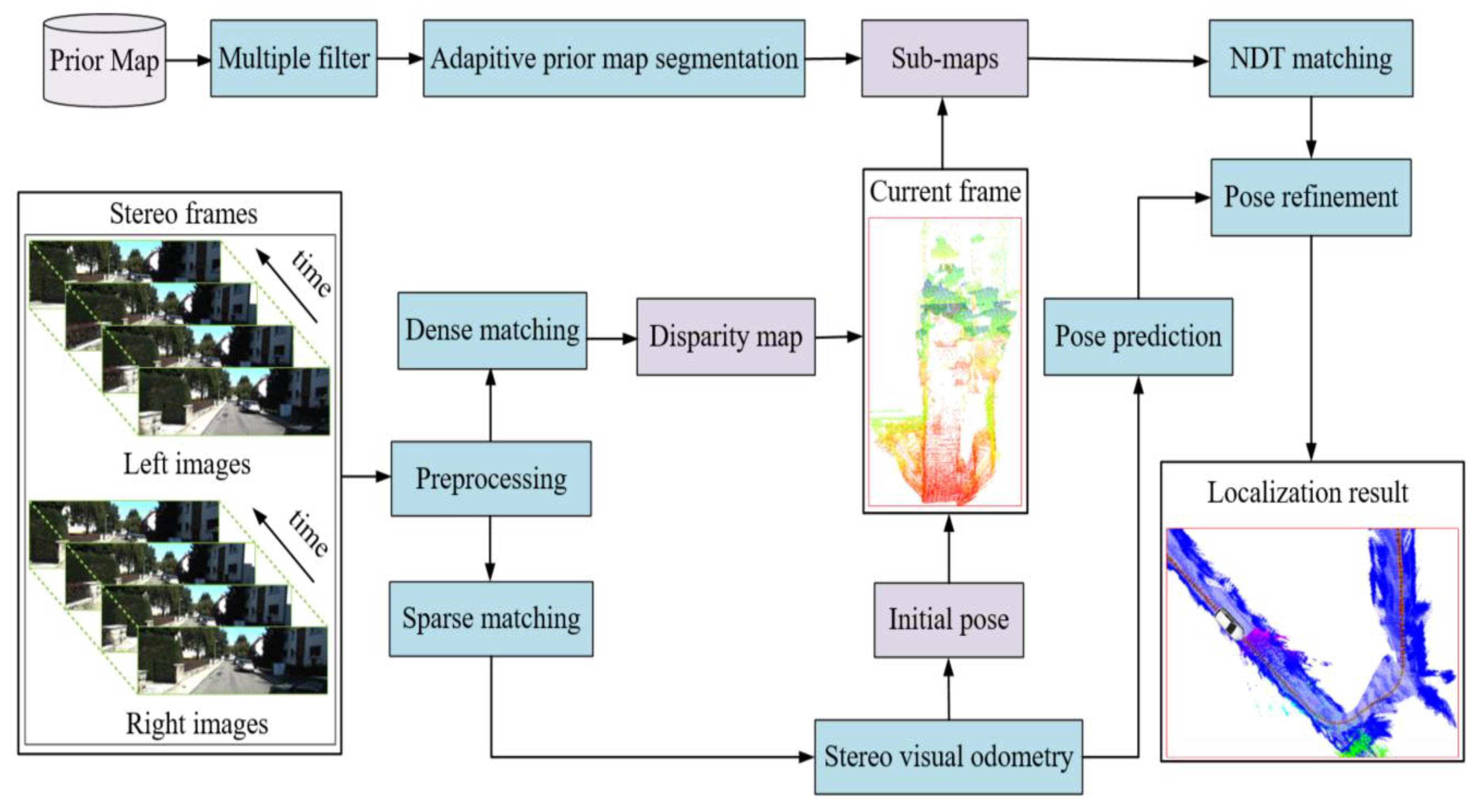
3. Methodology
3.1. Visual Point Cloud Generation
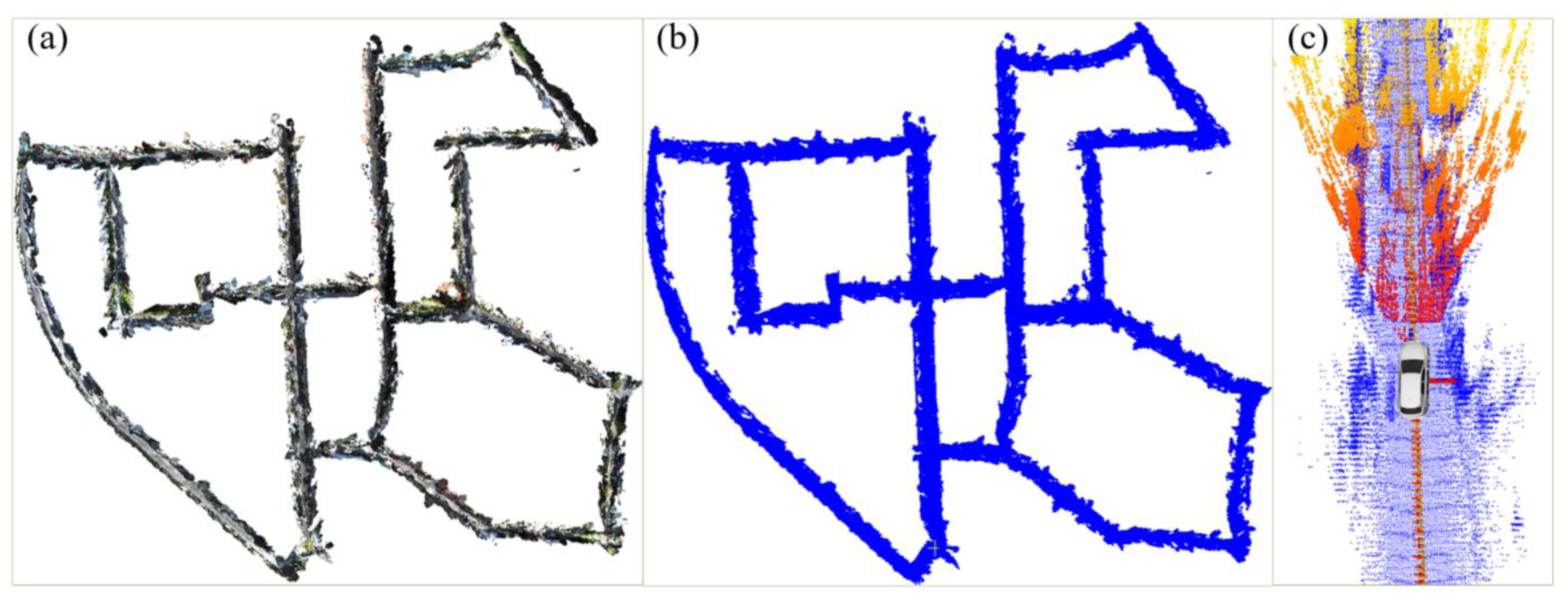
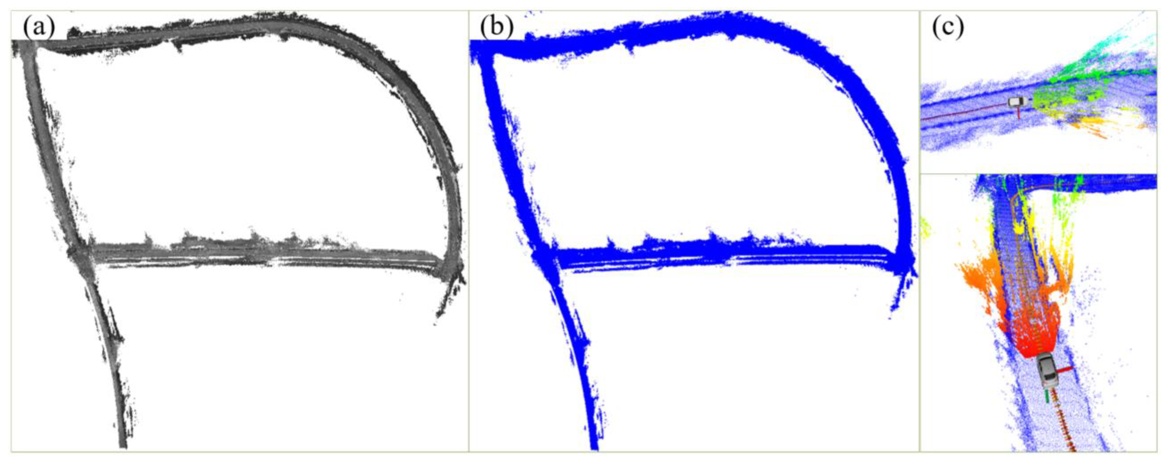
3.1.1. Priori Visual Point Cloud Map Generation
3.1.2. Multiple Filtering
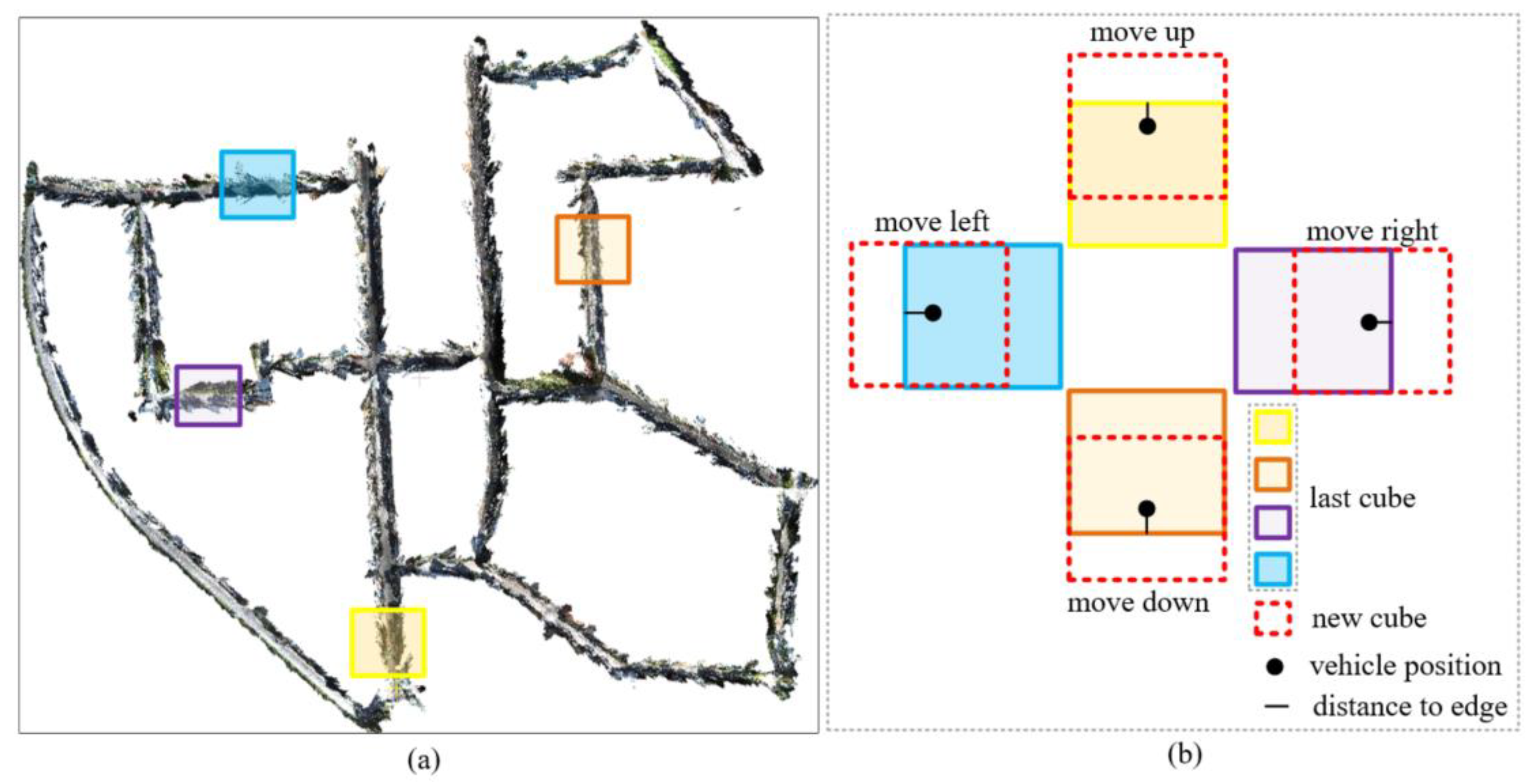
3.1.3. Adaptive Prior Map Segmentation
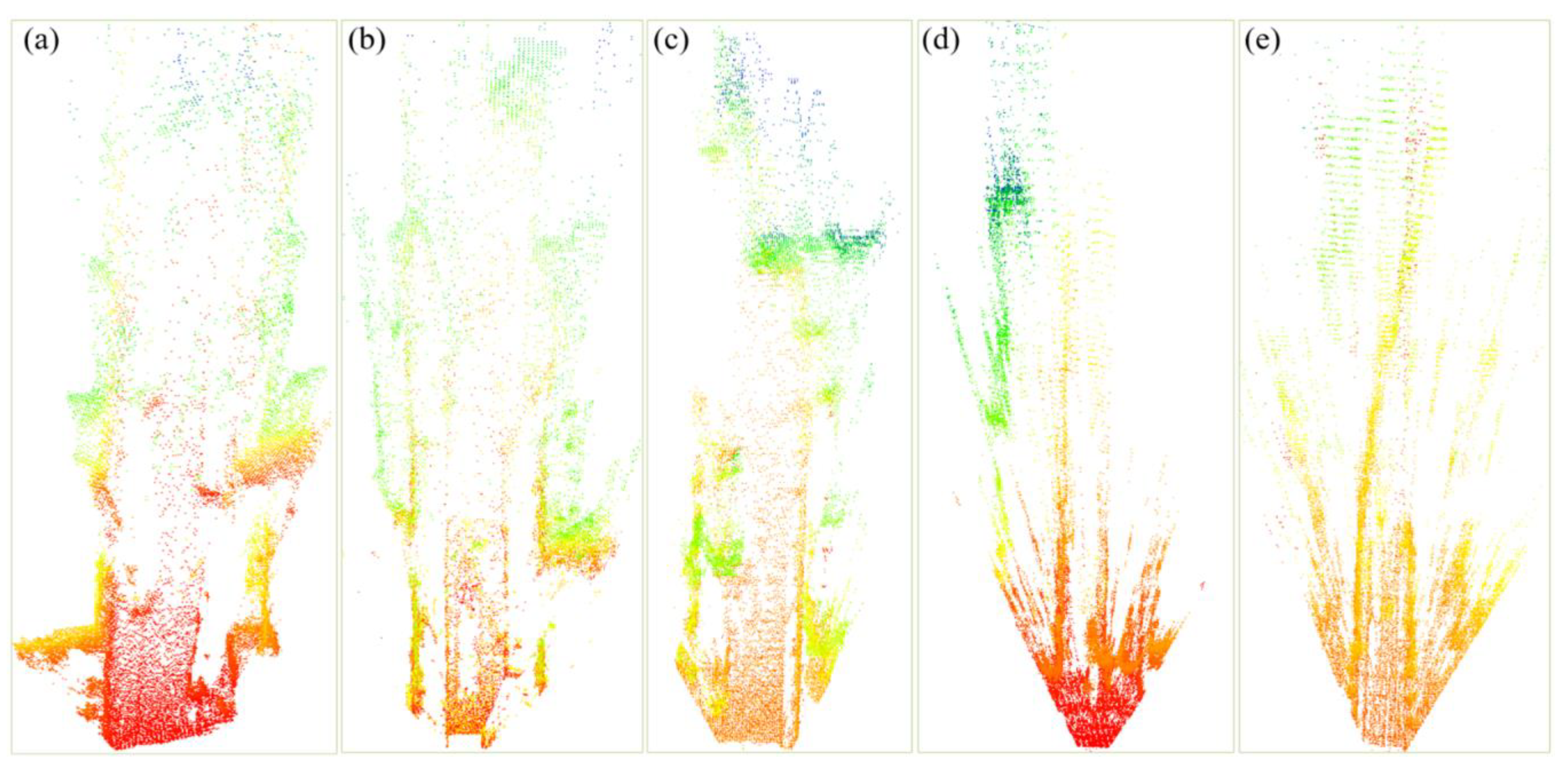
3.2. Current Visual Point Cloud Generation
3.3. Stereo Camera Localization with Prior Map Constraints
3.3.1. Initialization with Stereo Visual Odometry
3.3.2. NDT Matching and Localization Refinement
| Algorithm 1. The procedure of localization with prior visual point cloud map constraints |
| Input: prior dense visual point cloud map , sequence stereo images at 10 Hz. Output: refined pose between sequence frames, where . 1: data preprocessing to get compact priori visual point cloud map ; 2: multiple filtering and adaptive priori maps segmentation are performed on ; 3: for each pair of stereo images 4: do 5: rectified each pair of stereo images to get ; 6: dense stereo matching by SGBM to generate disparity map ; 7: convert disparity map to visual point cloud by formula (3-4); 8: estimate initial pose from stereo visual odometry based on ORB-SLAM2 framework; 9: If is initialized 10: make pose prediction based on the last frame ; 11: perform NDT matching between the current visual point cloud and the candidate sub-map to get the relative transformation ; 12: else 13: reinitialize ; 14: end for 15: update current pose by relative transformation parameters ; 16: return 17: refined pose between frames . |
4. Experimental Results
4.1. Experimental Platform Configuration
4.2. Qualitative Analysis
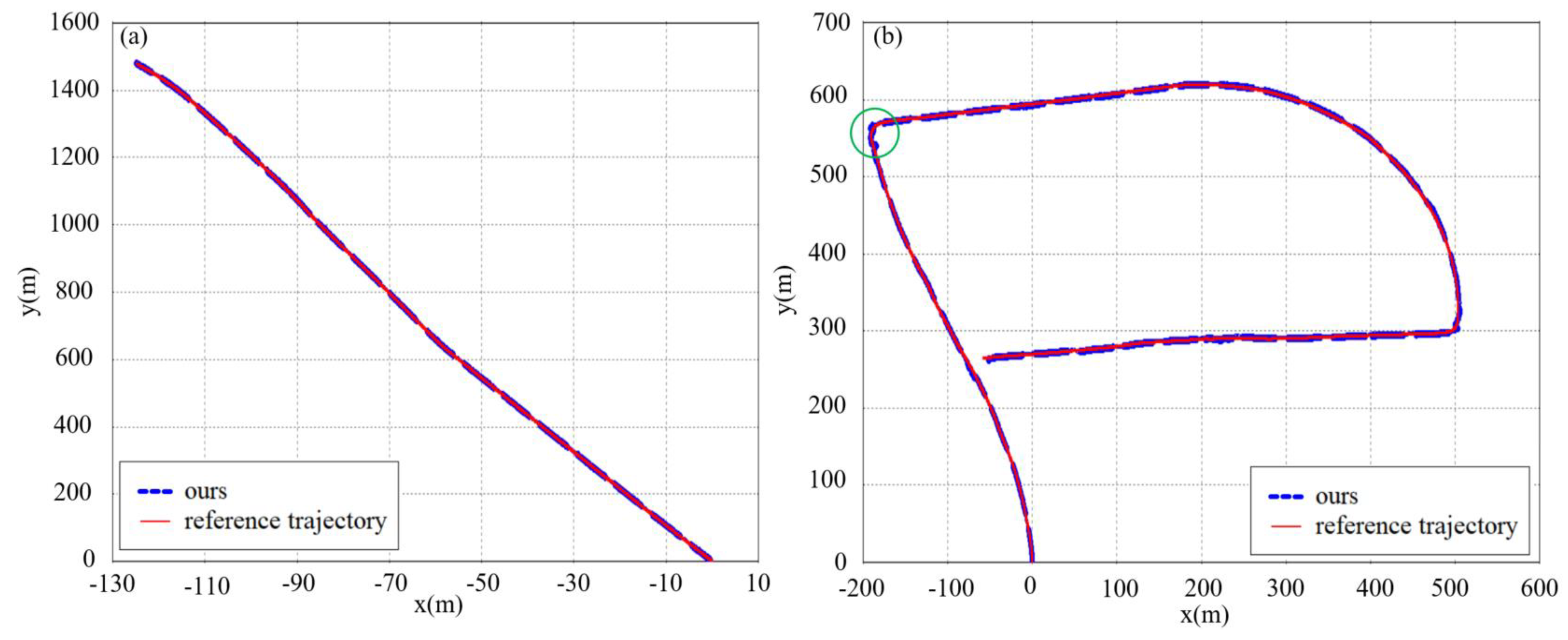
4.2.1. Evaluation with KITTI Dataset
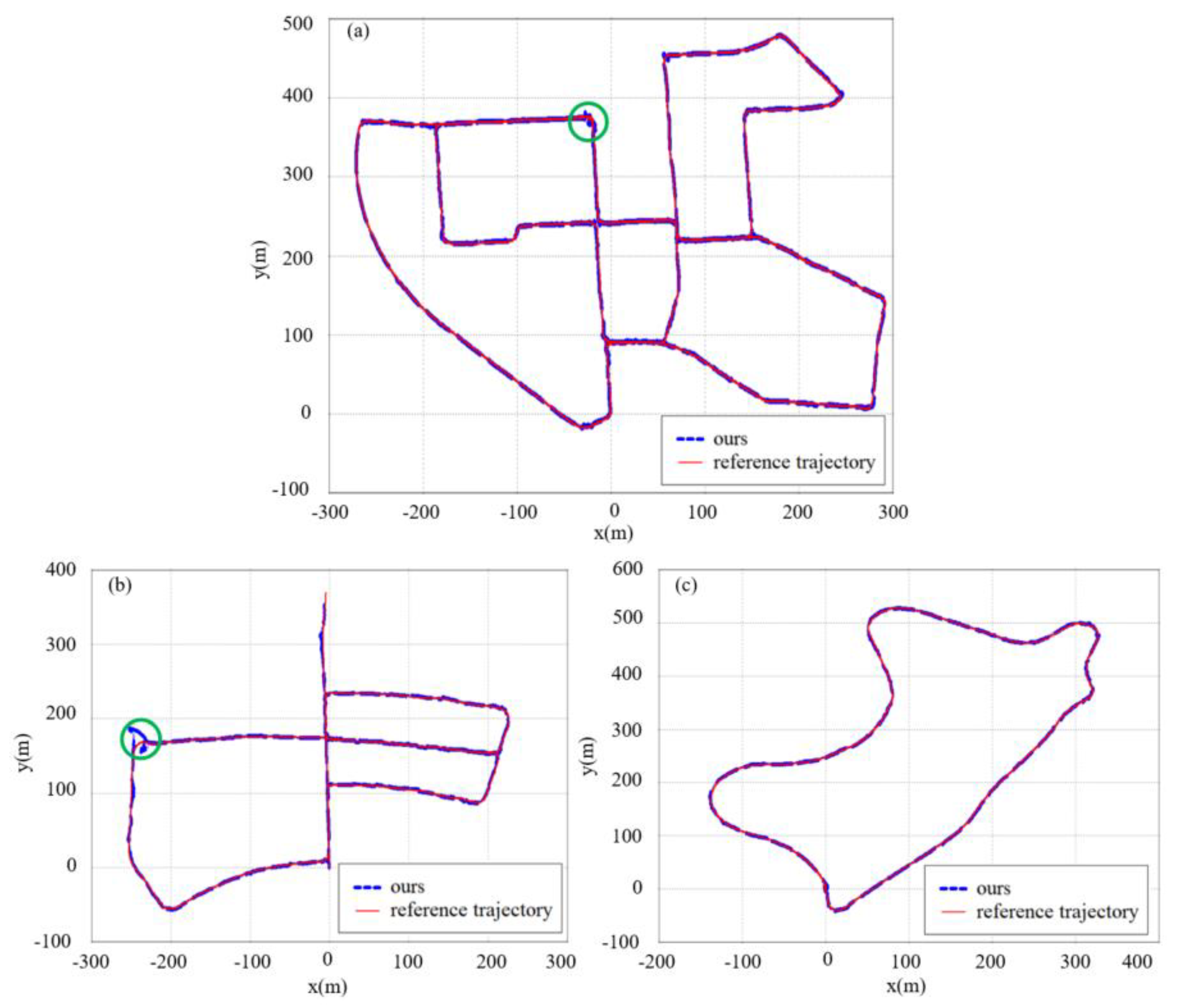
4.2.2. Evaluation with Field Test
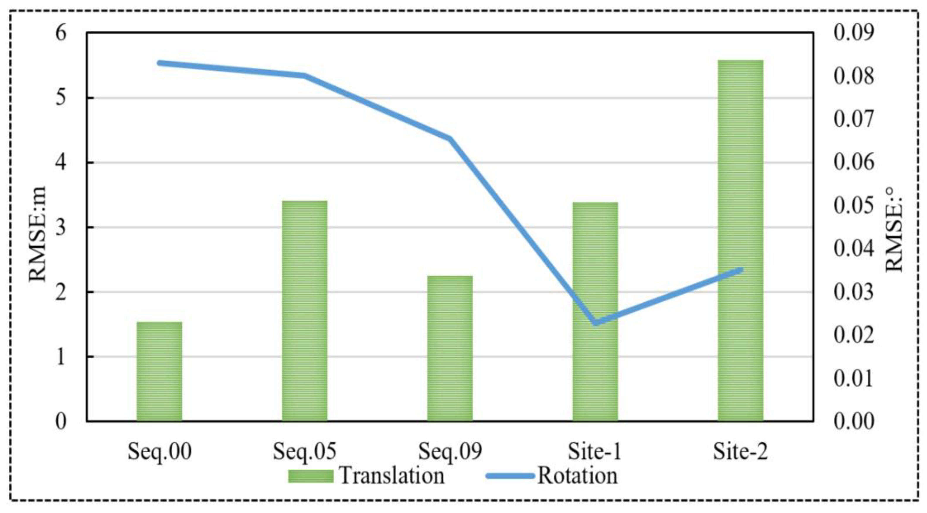
4.3. Quantitative Evaluation
4.4. Comparison with Other Methods
4.4.1. Comparison with Camera-Based Method
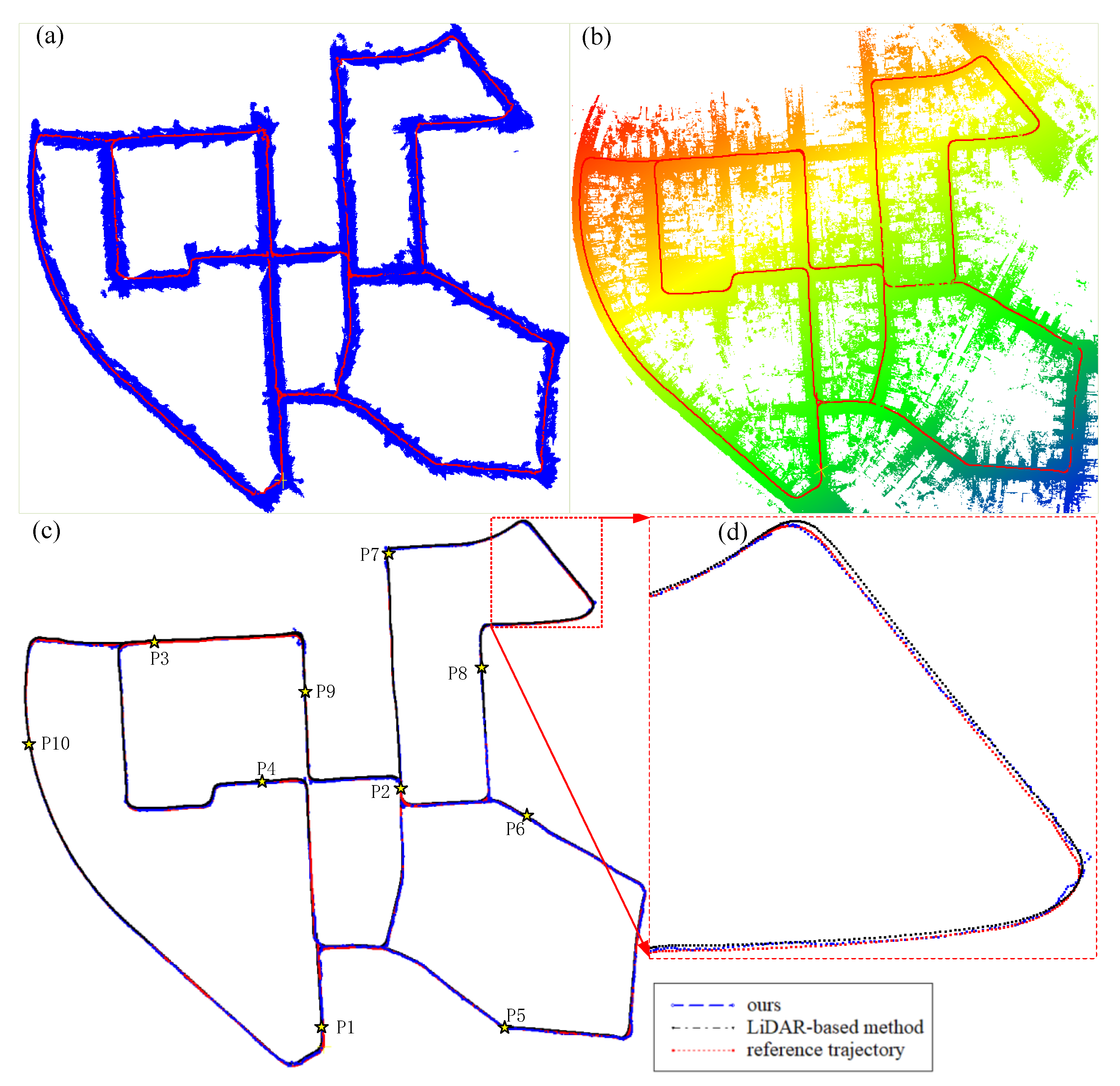
4.4.2. Comparison with LiDAR-Based Method
4.5. Time Performance
5. Discussion
6. Conclusions
Author Contributions
Funding
Institutional Review Board Statement
Informed Consent Statement
Data Availability Statement
Conflicts of Interest
References
- Wen, W.; Hsu, L.-T.; Zhang, G. Performance Analysis of NDT-based Graph SLAM for Autonomous Vehicle in Diverse Typical Driving Scenarios of Hong Kong. Sensors 2018, 18, 3928. [Google Scholar] [CrossRef] [PubMed]
- Carvalho, H.; Del Moral, P.; Monin, A.; Salut, G. Optimal nonlinear filtering in GPS/INS integration. IEEE Trans. Aerospace Electron. Syst. 1997, 33, 835–850. [Google Scholar] [CrossRef]
- Mohamed, A.H.; Schwarz, K.P. Adaptive kalman filtering for INS/GPS. J. Geodesy 1999, 73, 193–203. [Google Scholar] [CrossRef]
- Wang, D.; Xu, X.; Zhu, Y. A Novel Hybrid of a Fading Filter and an Extreme Learning Machine for GPS/INS during GPS Outages. Sensors 2018, 18, 3863. [Google Scholar] [CrossRef] [PubMed]
- Liu, H.; Ye, Q.; Wang, H.; Chen, L.; Yang, J. A Precise and Robust Segmentation-Based Lidar Localization System for Automated Urban Driving. Remote Sens. 2019, 11, 1348. [Google Scholar] [CrossRef]
- Nuchter, A.; Lingemann, K.; Hertzberg, J.; Surmann, H. 6D SLAM-3D mapping outdoor environments. J. Field Robot. 2007, 24, 699–722. [Google Scholar] [CrossRef]
- Bosse, M.; Zlot, R.; Flick, P. Zebedee: Design of a spring-mounted 3-d range sensor with application to mobile mapping. IEEE Trans. Robot. 2012, 28, 1104–1119. [Google Scholar] [CrossRef]
- Suzuki, T.; Kitamura, M.; Amano, Y.; Hashizume, T. 6-DOF localization for a mobile robot using outdoor 3D voxel maps. In Proceedings of the 2010 IEEE/RSJ International Conference on Intelligent Robots and Systems (IROS), Taipei, Taiwan, 18–22 October 2010; pp. 5737–5743. [Google Scholar]
- Yoneda, K.; Tehrani, H.; Ogawa, T.; Hukuyama, N.; Mita, S. Lidar scan feature for localization with highly precise 3-D map. In Proceedings of the 2014 IEEE Intelligent Vehicles Symposium, Dearborn, MI, USA, 8–11 June 2014; pp. 1345–1350. [Google Scholar]
- Ruchti, P.; Steder, B.; Ruhnke, M.; Burgard, W. Localization on openstreetmap data using a 3D laser scanner. In Proceedings of the 2016 IEEE International Conference on Robotics and Automation (ICRA), Seattle, WA, USA, 26–30 May 2015; pp. 5260–5265. [Google Scholar]
- Stewart, A.D.; Newman, P. LAPS-localisation using appearance of prior structure: 6-dof monocular camera localisation using prior pointclouds. In Proceedings of the 2012 IEEE International Conference on Robotics and Automation (ICRA), Saint Paul, MN, USA, 14–18 May 2012; pp. 2625–2632. [Google Scholar]
- Wolcott, R.W.; Eustice, R.M. Visual localization within LIDAR maps for automated urban driving. In Proceedings of the 2014 IEEE/RSJ International Conference on Intelligent Robots and Systems (IROS), Chicago, IL, USA, 14–18 September 2014; pp. 176–183. [Google Scholar]
- Li, Q.; Zhu, J.S.; Liu, J.; Cao, R.; Fu, H.; Garibaldi, J.M.; Li, Q.Q.; Liu, B.Z.; Qiu, G.P. 3D map-guided single indoor image localization refinement. ISPRS J. Photogramm. Remote Sens. 2020, 161, 13–26. [Google Scholar] [CrossRef]
- Neubert, P.; Schubert, S.; Protzel, P. Sampling-based methods for visual navigation in 3D maps by synthesizing depth images. In Proceedings of the 2017 IEEE/RSJ International Conference on Intelligent Robots and Systems (IROS), Vancouver, BC, Canada, 24–28 September 2017; pp. 2492–2498. [Google Scholar]
- Xu, Y.Q.; John, V.; Mita, S.; Tehrani, H.; Ishimaru, K.; Nishino, S. 3D point cloud map based vehicle localization using stereo camera. In Proceedings of the 2017 IEEE Intelligent Vehicles Symposium (IV), Los Angeles, CA, USA, 11–14 June 2017; pp. 487–492. [Google Scholar]
- Geiger, A.; Lenz, P.; Urtasun, R. Are we ready for autonomous driving? The KITTI vision benchmark suite. In Proceedings of the 2012 IEEE Computer Society Conference on Computer Vision and Pattern Recognition (CVPR), Providence, RI, USA, 16–21 June 2012; pp. 3354–3361. [Google Scholar]
- Choi, J. Hybrid map-based SLAM using a Velodyne laser scanner. In Proceedings of the 17th International IEEE Conference on Intelligent Transportation Systems (ITSC), Qingdao, China, 8–11 October 2014; pp. 3082–3087. [Google Scholar]
- Im, J.H.; Im, S.-H.; Jee, G.I. Vertical corner feature based precise vehicle localization using 3D LIDAR in urban area. Sensors 2016, 16, 1268. [Google Scholar] [CrossRef] [PubMed]
- Levinson, J.; Montemerlo, M.; Thrun, S. Map-based precision vehicle localization in urban environments. In Proceedings of the Robotics: Science and Systems III, Atlanta, GA, USA, 27–30 June 2007; p. 1. [Google Scholar]
- Levinson, J.; Thrun, S. Robust vehicle localization in urban environments using probabilistic maps. In Proceedings of the 2010 IEEE International Conference on Robotics and Automation (ICRA), Anchorage, AK, USA, 3–7 May 2010; pp. 4372–4378. [Google Scholar]
- Kim, D.; Chung, T.; Yi, K. Lane map building and localization for automated driving using 2D laser rangefinder. In Proceedings of the 2015 IEEE Intelligent Vehicles Symposium (IV), Seoul, Korea, 28 June–1 July 2015; pp. 680–685. [Google Scholar]
- Qin, B.; Chong, Z.J.; Bandyopadhyay, T.; Ang, M.H.; Frazzoli, E.; Rus, D. Curb-intersection feature based Monte Carlo Localization on urban roads. In Proceedings of the 2012 IEEE International Conference on Robotics and Automation (ICRA), Saint Paul, MN, USA, 14–18 May 2012; pp. 2640–2646. [Google Scholar]
- Forster, C.; Pizzoli, M.; Scaramuzza, D. Air-ground localization and map augmentation using monocular dense reconstruction. In Proceedings of the 2013 IEEE/RSJ International Conference on Intelligent Robots and Systems (IROS), Tokyo, Japan, 3–7 November 2013; pp. 3971–3978. [Google Scholar]
- Steder, B.; Ruhnke, M.; Burgard, W. Monocular camera localization in 3D lidar maps. In Proceedings of the 2016 IEEE/RSJ International Conference on Intelligent Robots and Systems (IROS), Daejeon, Korea, 9–14 October 2016; pp. 1926–1931. [Google Scholar]
- Brubaker, M.A.; Geiger, A.; Urtasun, R. Map-based probabilistic visual self-localization. IEEE Trans. Pattern Anal. Mach. Intell. 2016, 38, 652–665. [Google Scholar] [CrossRef] [PubMed]
- Ziegler, J.; Lategahn, H.; Schreiber, M.; Keller, C.G.; Knöppel, C.; Hipp, J.; Haueis, M.; Stiller, C. Video based localization for bertha. In Proceedings of the 2014 IEEE Intelligent Vehicles Symposium Proceedings, Dearborn, MI, USA, 8–11 June 2014; pp. 1231–1238. [Google Scholar]
- Radwan, N.; Tipaldi, G.D.; Spinello, L.; Burgard, W. Do you see the bakery? Leveraging geo-referenced texts for global localization in public maps. In Proceedings of the 2016 IEEE international conference on robotics and automation (ICRA), Stockholm, Sweden, 16–21 May 2016; pp. 4837–4842. [Google Scholar]
- Spangenberg, R.; Goehring, D.; Rojas, R. Pole-based localization for autonomous vehicles in urban scenarios. In Proceedings of the 2016 IEEE/RSJ International Conference on Intelligent Robots and Systems (IROS), Daejeon, Korea, 9–14 October 2016; pp. 2161–2166. [Google Scholar]
- Lyrio, L.J.; Oliveira-Santos, T.; Badue, C.; De Souza, A.F. Image-based mapping, global localization and position tracking using vg-ram weightless neural networks. In Proceedings of the 2015 IEEE International Conference on Robotics and Automation (ICRA), Seattle, WA, USA, 26–30 May 2015; pp. 3603–3610. [Google Scholar]
- Oliveira, G.L.; Radwan, N.; Burgard, W.; Brox, T. Topometric localization with deep learning. arXiv 2017, arXiv:1706.08775. [Google Scholar]
- Lin, X.H.; Yang, B.S.; Wang, F.H.; Li, J.P.; Wang, X.Q. Dense 3D surface reconstruction of large-scale streetscape from vehicle-borne imagery and LiDAR. Int. J. Digit. Earth 2020, 1–21. [Google Scholar] [CrossRef]
- Chang, J.R.; Chen, Y.S. Pyramid stereo matching network. In Proceedings of the 2018 IEEE/CVF Conference on Computer Vision and Pattern Recognition (CVPR), Salt Lake City, UT, USA, 18–23 June 2018; pp. 5410–5418. [Google Scholar]
- Lin, X.H.; Wang, F.H.; Guo, L.; Zhang, W.W. An automatic key-frame selection method for monocular visual odometry of ground vehicle. IEEE Access 2019, 7, 70742–70754. [Google Scholar] [CrossRef]
- Rusu, R.B.; Cousins, S. 3D is here: Point cloud library (PCL). In Proceedings of the 2011 IEEE International Conference on Robotics and Automation (ICRA), Shanghai, China, 9–13 May 2011; pp. 1–4. [Google Scholar]
- Kim, H.; Liu, B.; Goh, C.Y.; Lee, S.; Myung, H. Robust Vehicle Localization Using Entropy-Weighted Particle Filter-based Data Fusion of Vertical and Road Intensity Information for a Large Scale Urban Area. IEEE Robot. Autom. Lett. 2017, 2, 1518–1524. [Google Scholar] [CrossRef]
- Hirschmuller, H. Stereo Processing by Semiglobal Matching and Mutual Information. IEEE Trans. Pattern Anal. Mach. Intell. 2008, 30, 328–341. [Google Scholar] [CrossRef] [PubMed]
- Scaramuzza, D.; Fraundorfer, F. Visual odometry: Part I, the first 30 years and fundamentals. IEEE Robotics and Automation Magazine. 2011, 18, 80–91. [Google Scholar] [CrossRef]
- Mur-Artal, R.; Tardós, J.D. Orb-slam2: An open-source slam system for monocular, stereo, and rgb-d cameras. IEEE Trans. Robot. 2017, 33, 1255–1262. [Google Scholar] [CrossRef]
- Kuemmerle, R.; Grisetti, G.; Strasdat, H.; Konolige, K.; Burgard, W. g2o: A general framework for graph optimization. In Proceedings of the 2011 IEEE international conference on robotics and automation (ICRA), Shanghai, China, 9–13 May 2011; pp. 3607–3613. [Google Scholar]
- Huhle, B.; Magnusson, M.; Straßer, W.; Lilienthal, A.J. Registration of colored 3d point clouds with a kernel-based extension to the normal distributions transform. In Proceedings of the 2008 IEEE international conference on robotics and automation (ICRA), Pasadena, CA, USA, 19–23 May 2008; pp. 4025–4030. [Google Scholar]
- Magnusson, M.; Nuchter, A.; Lorken, C.; Lilienthal, A.J.; Hertzberg, J. Evaluation of 3d registration reliability and speed-a comparison of ICP and NDT. In Proceedings of the 2009 IEEE international conference on robotics and automation (ICRA), Kobe, Japan, 12–17 May 2009; pp. 3907–3912. [Google Scholar]
- Magnusson, M. The Three-Dimensional Normal-Distributions Transform: An Efficient Representation for Registration, Surface Analysis, and Loop Detection. Ph.D. Thesis, Örebro University, Örebro, Sweden, 2013. [Google Scholar]
- Zhang, Z.; Scaramuzza, D. A Tutorial on Quantitative Trajectory Evaluation for Visual (-Inertial) Odometry. In Proceedings of the 2018 IEEE/RSJ International Conference on Intelligent Robots and Systems (IROS), Madrid, Spain, 1–5 October 2018; pp. 7244–7251. [Google Scholar]
- Sturm, J.; Engelhard, N.; Endres, F.; Burgard, W.; Cremers, D. A benchmark for the evaluation of RGB-D SLAM systems. In Proceedings of the 2012 IEEE/RSJ international conference on intelligent robots and systems (IROS), Vilamoura, Portugal, 7–12 October 2012; pp. 573–580. [Google Scholar]
- Kim, Y.J.; Jeong, J.Y.; Kim, A. Stereo Camera Localization in 3D LiDAR Maps. In Proceedings of the 2018 IEEE/RSJ International Conference on Intelligent Robots and Systems (IROS), Madrid, Spain, 1–5 October 2018; pp. 1–9. [Google Scholar]
- Shan, T.; Englot, B. LeGO-LOAM: Lightweight and Ground-Optimized Lidar Odometry and Mapping on Variable Terrain. In Proceedings of the 2018 IEEE/RSJ International Conference on Intelligent Robots and Systems (IROS), Madrid, Spain, 1–5 October 2018; pp. 4758–4765. [Google Scholar]


| Scene | Ours | Kim et al. [45] | ||||||
|---|---|---|---|---|---|---|---|---|
| Translation/m | Rotation/° | Translation/m | Rotation/° | |||||
| Average | Std. | Average | Std. | Average | Std. | Average | Std. | |
| 00 | 1.27 | 0.93 | 1.20 | 2.03 | 0.13 | 0.11 | 0.32 | 0.39 |
| 05 | 3.18 | 5.58 | 1.27 | 1.97 | 0.15 | 0.14 | 0.34 | 0.40 |
| 09 | 1.94 | 1.22 | 1.06 | 1.61 | 0.18 | 0.22 | 0.34 | 0.34 |
| Methods | Segments Horizontal Localization Errors (m) | ||||||||||
|---|---|---|---|---|---|---|---|---|---|---|---|
| P1 | P2 | P3 | P4 | P5 | P6 | P7 | P8 | P9 | P10 | Average | |
| Ours | 1.04 | 0.33 | 1.82 | 1.59 | 0.74 | 1.24 | 2.96 | 0.56 | 0.63 | 0.25 | 1.12 |
| LiDAR-based method | 1.60 | 0.25 | 1.45 | 1.73 | 1.38 | 0.95 | 0.87 | 0.35 | 0.32 | 0.44 | 0.93 |
| Sequences | Length (m) | Image Size | IPE (s) | CVPCG (s) | APMS (s) | DSDC (s) | Localization (s) | Average (s) |
|---|---|---|---|---|---|---|---|---|
| 00 | 3723.30 | 1241 × 376 | 0.12 | 0.15 | 0.02 | 0.11 | 0.33 | 0.73 |
| 05 | 2203.91 | 1226 × 370 | 0.11 | 0.14 | 0.01 | 0.11 | 0.33 | 0.70 |
| 09 | 1704.76 | 1226 × 370 | 0.11 | 0.12 | 0.01 | 0.10 | 0.33 | 0.67 |
| Site-1 | 1550.53 | 1280 × 640 | 0.08 | 0.23 | 0.01 | 0.21 | 0.34 | 0.87 |
| Site-2 | 2248.42 | 1280 × 640 | 0.08 | 0.24 | 0.01 | 0.20 | 0.35 | 0.88 |
Publisher’s Note: MDPI stays neutral with regard to jurisdictional claims in published maps and institutional affiliations. |
© 2021 by the authors. Licensee MDPI, Basel, Switzerland. This article is an open access article distributed under the terms and conditions of the Creative Commons Attribution (CC BY) license (http://creativecommons.org/licenses/by/4.0/).
Share and Cite
Lin, X.; Wang, F.; Yang, B.; Zhang, W. Autonomous Vehicle Localization with Prior Visual Point Cloud Map Constraints in GNSS-Challenged Environments. Remote Sens. 2021, 13, 506. https://doi.org/10.3390/rs13030506
Lin X, Wang F, Yang B, Zhang W. Autonomous Vehicle Localization with Prior Visual Point Cloud Map Constraints in GNSS-Challenged Environments. Remote Sensing. 2021; 13(3):506. https://doi.org/10.3390/rs13030506
Chicago/Turabian StyleLin, Xiaohu, Fuhong Wang, Bisheng Yang, and Wanwei Zhang. 2021. "Autonomous Vehicle Localization with Prior Visual Point Cloud Map Constraints in GNSS-Challenged Environments" Remote Sensing 13, no. 3: 506. https://doi.org/10.3390/rs13030506
APA StyleLin, X., Wang, F., Yang, B., & Zhang, W. (2021). Autonomous Vehicle Localization with Prior Visual Point Cloud Map Constraints in GNSS-Challenged Environments. Remote Sensing, 13(3), 506. https://doi.org/10.3390/rs13030506