
Wetland Mapping Using HJ-1A/B Hyperspectral Images and an Adaptive Sparse Constrained Least Squares Linear Spectral Mixture Model


Abstract

1. Introduction
2. Study Site and Materials
2.1. Study Site
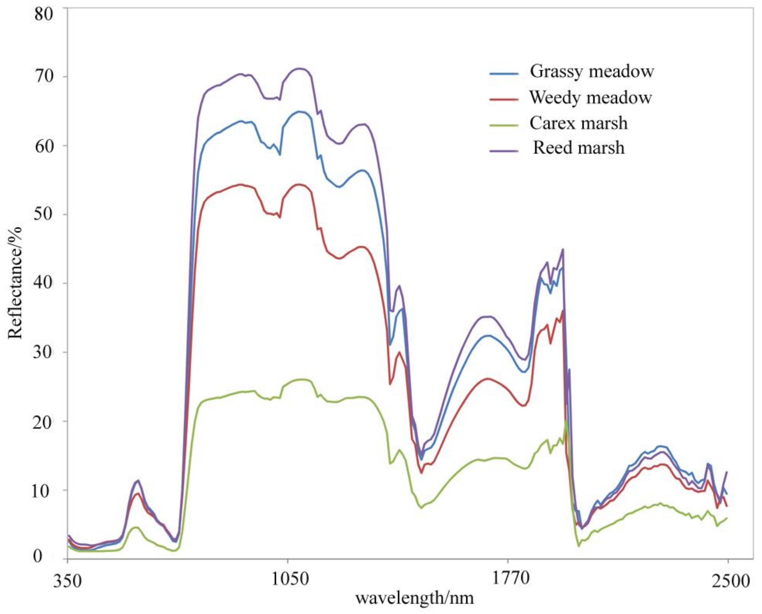
2.2. Materials
3. Method
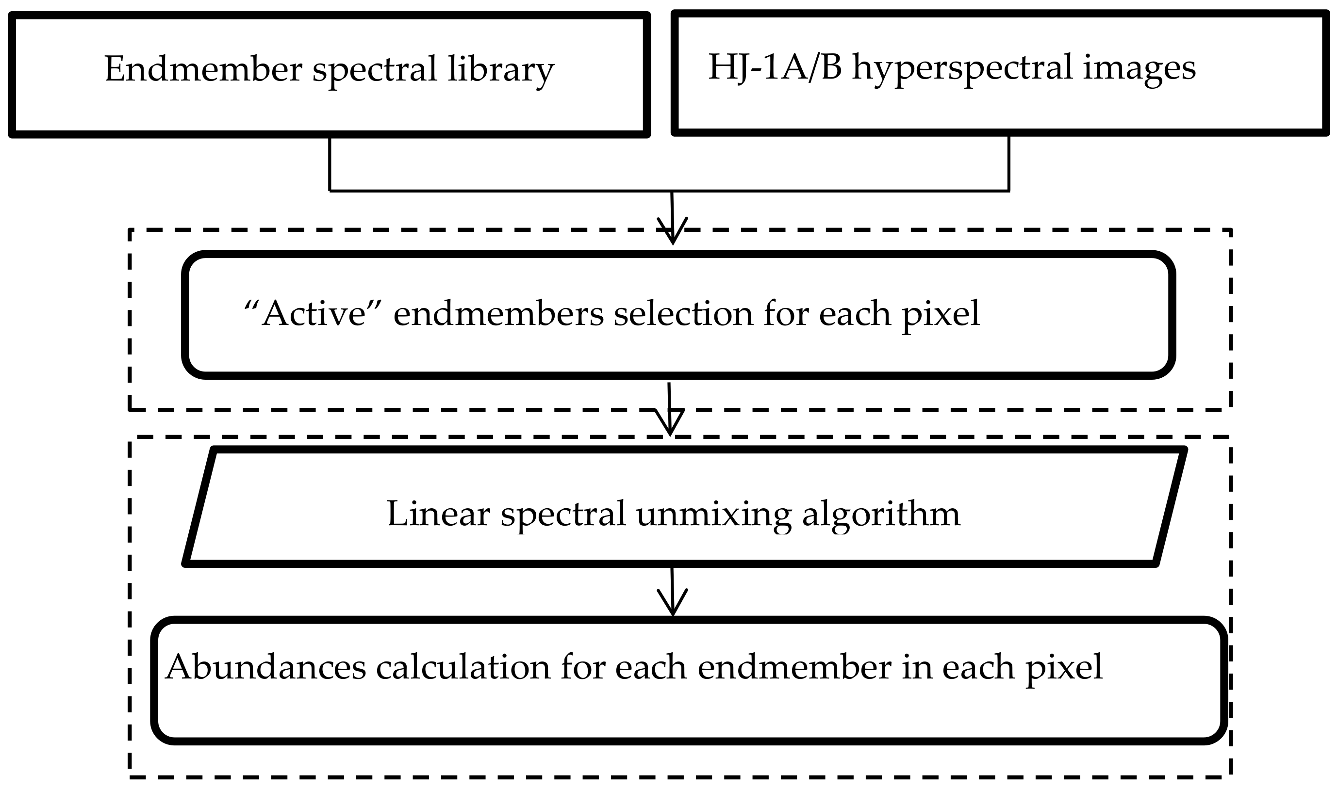
3.1. Adaptive Endmembers Selection Based on Sparsity Constrained Method
3.2. Abundance Inversion Based on Linear Spectral Mixture Model
3.3. The Accuracy Evaluations of Two LSMMs
4. Results
4.1. Classification Results Based on SCLS-LSMM
4.2. Accuracy Assessment and Comparative Analysis
5. Discussion
6. Conclusions
Author Contributions
Funding
Data Availability Statement
Acknowledgments
Conflicts of Interest
References
- Mitsch, W.; Gosselink, J. Wetlands, 3rd ed.; Van Nostrand Reinhold: New York, NY, USA, 1993. [Google Scholar]
- Na, X.D.; Zang, S.; Zhang, Y.H.; Li, W. Assessing Breeding Habitat Suitability for the Endangered red-Crowned Crane (Grus japonensis) Based on Multi-Source Remote Sensing Data. Wetlands 2015, 35, 955–967. [Google Scholar] [CrossRef]
- Finlayson, M.; Cruz, R.D.; Davidson, N.; Alder, J.; Cork, S.; Groot, R.S.D.; Lévêque, C.; Milton, G.R.; Peterson, G.; Pritchard, G. Millennium Ecosystem Assessment: Ecosystems and human well-being: Wetlands and water synthesis. Data Fusion Concepts Ideas 2005, 656, 87–98. [Google Scholar]
- Park, H.; Kim, Y.; Kimball, J.S. Widespread permafrost vulnerability and soil active layer increases over the high northern latitudes inferred from satellite remote sensing and process model assessments. Remote Sens. Environ. 2016, 175, 349–358. [Google Scholar] [CrossRef]
- Rundquist, D.C.; Narumalani, S.; Narayanan, R.M. A review of wetlands remote sensing and defining new considerations. Remote Sens. Rev. 2001, 20, 207–226. [Google Scholar] [CrossRef]
- Baker, C.; Lawrence, R.; Montagne, C.; Patten, D. Mapping wetlands and riparian areas using Landsat ETM+ imagery and decision-tree-based models. Wetlands 2006, 26, 465–474. [Google Scholar] [CrossRef]
- Davranche, A.; Lefebvre, G.; Poulin, B. Wetland monitoring using classification trees and SPOT-5 seasonal time series. Remote Sens. Environ. 2010, 114, 552–562. [Google Scholar] [CrossRef]
- Han, X.; Chen, X.; Feng, L. Four decades of winter wetland changes in Poyang Lake based on Landsat observations be-tween 1973 and 2013. Remote Sens. Environ. 2015, 156, 426–437. [Google Scholar] [CrossRef]
- Stehman, S.; Wickham, J.; Smith, J.; Yang, L. Thematic accuracy of the 1992 National Land-Cover Data for the eastern United States: Statistical methodology and regional results. Remote Sens. Environ. 2003, 86, 500–516. [Google Scholar] [CrossRef]
- Lang, M.W.; Kasischke, E.S.; Prince, S.D.; Pittman, K.W. Assessment of C-band synthetic aperture radar data for map-ping and monitoring Coastal Plain forested wetlands in the Mid-Atlantic Region, U.S.A. Remote Sens. Environ. 2008, 112, 4120–4130. [Google Scholar] [CrossRef]
- Bwangoy, J.-R.B.; Hansen, M.C.; Roy, D.P.; De Grandi, G.; Justice, C.O. Wetland mapping in the Congo Basin using optical and radar remotely sensed data and derived topographical indices. Remote Sens. Environ. 2010, 114, 73–86. [Google Scholar] [CrossRef]
- Na, X.D.; Zang, S.Y.; Wu, C.S.; Li, W.L. Mapping forested wetlands in the Great Zhan River Basin through integrating optical, radar, and topographical data classification techniques. Environ. Monit. Assess. 2015, 187, 696. [Google Scholar] [CrossRef]
- Na, X.; Zhang, S.; Li, X.; Yu, H.; Liu, C. Improved Land Cover Mapping using Random Forests Combined with Landsat Thematic Mapper Imagery and Ancillary Geographic Data. Photogramm. Eng. Remote Sens. 2010, 76, 833–840. [Google Scholar] [CrossRef]
- Chen, B.; Chen, L.; Lu, M.; Xu, B. Wetland mapping by fusing fine spatial and hyperspectral resolution images. Ecol. Model. 2017, 353, 95–106. [Google Scholar] [CrossRef]
- Pengra, B.W.; Johnston, C.A.; Loveland, T.R. Mapping an invasive plant, Phragmites australis, in coastal wetlands us-ing the EO-1 Hyperion hyperspectral sensor. Remote Sens. Environ. 2007, 108, 74–81. [Google Scholar] [CrossRef]
- Beland, M.; Roberts, D.A.; Peterson, S.H.; Biggs, T.W.; Kokaly, R.F.; Piazza, S.; Roth, K.L.; Khanna, S.; Ustin, S.L. Mapping changing distributions of dominant species in oil-contaminated salt marshes of Louisiana using imaging spectroscopy. Remote Sens. Environ. 2016, 182, 192–207. [Google Scholar] [CrossRef]
- Onojeghuo, A.O.; Blackburn, G.A. Optimising the use of hyperspectral and LiDAR data for mapping reedbed habitats. Remote Sens. Environ. 2011, 115, 2025–2034. [Google Scholar] [CrossRef]
- Zorner, R.J.; Trabucco, A.; Ustin, S.L. Building spectral libraries for wetlands land cover classification and hyperspectral remote sensing. J. Environ. Manag. 2009, 90, 2170–2177. [Google Scholar]
- Harris, A.; Charnock, R.; Lucas, R. Hyperspectral remote sensing of peatland floristic gradients. Remote Sens. Environ. 2015, 162, 99–111. [Google Scholar] [CrossRef]
- Fu, B.L.; Wang, Y.Q.; Campbell, A.; Li, Y.; Zhang, B.; Yin, S.B.; Xing, Z.F.; Jin, X.M. Comparison of object-based and pix-el-based Random Forest algorithm for wetland vegetation mapping using high spatial resolution GF-1 and SAR data. Ecol. Indic. 2017, 73, 105–117. [Google Scholar] [CrossRef]
- Onojeghuo, A.O.; Onojeghuo, A.R. Object-based habitat mapping using very high spatial resolution multispectral and hyperspectral imagery with LiDAR data. Int. J. Appl. Earth Obs. Geoinf. 2017, 59, 79–91. [Google Scholar] [CrossRef]
- Hestir, E.L.; Khanna, S.K.; Andrew, M.E.; Santos, M.J.; Viers, J.H.; Greenberg, J.A.; Rajapakse, S.S.; Ustin, S.L. Identification of invasive vegetation using hyperspectral remote sensing in the California Delta ecosystem. Remote Sens. Environ. 2008, 112, 4034–4047. [Google Scholar] [CrossRef]
- Bian, J.; Li, A.; Zhang, Z.; Zhao, W.; Lei, G.; Yin, G.; Jin, H.; Tan, J.; Huang, C. Monitoring fractional green vegetation cover dynamics over a seasonally inundated alpine wetland using dense time series HJ-1A/B constellation images and an adaptive endmember selection LSMM model. Remote Sens. Environ. 2017, 197, 98–114. [Google Scholar] [CrossRef]
- Small, C. Estimation of urban vegetation abundance by spectral mixture analysis. Int. J. Remote Sens. 2001, 22, 1305–1334. [Google Scholar] [CrossRef]
- Michishita, R.; Jiang, Z.B.; Gong, P.; Xu, B. Bi-scale analysis of multitemporal land cover fractions for wetland vegetation mapping. ISPRS J. Photogram. Remote Sens. 2012, 72, 1–15. [Google Scholar] [CrossRef]
- Roberts, D.A.; Dennison, P.E.; Roth, K.L.; Dudley, K.; Hulley, G.C. Relationships between dominant plant species, fractional cover and Land Surface Temperature in a Mediterranean ecosystem. Remote Sens. Environ. 2015, 167, 152–167. [Google Scholar] [CrossRef]
- Meng, R.; Wu, J.; Schwager, K.L.; Zhao, F.; Dennison, P.E.; Cook, B.D.; Brewster, K.; Green, T.M.; Serbin, S.P. Using high spa-tial resolution satellite imagery to map forest burn severity across spatial scales in a Pine Barrens ecosystem. Remote Sens. Environ. 2017, 191, 95–109. [Google Scholar] [CrossRef]
- DeFries, R.; Hansen, M.; Townshend, J.; Janetos, A.; Loveland, T. A new global 1-km dataset of percentage tree cover derived from remote sensing. Glob. Chang. Biol. 2001, 6, 247–254. [Google Scholar] [CrossRef]
- Degerickx, J.; Roberts, D.; Somers, B. Enhancing the performance of Multiple Endmember Spectral Mixture Analysis (MESMA) for urban land cover mapping using airborne lidar data and band selection. Remote Sens. Environ. 2019, 221, 260–273. [Google Scholar] [CrossRef]
- Rahmani, S.; Strait, M.; Merkurjev, D.; Moeller, M.; Wittman, T. An Adaptive IHS Pan-Sharpening Method. IEEE Geosci. Remote Sens. Lett. 2010, 7, 746–750. [Google Scholar] [CrossRef]
- Iordache, M.-D.; Bioucas-Dias, J.M.; Plaza, A. Sparse Unmixing of Hyperspectral Data. IEEE Trans. Geosci. Remote Sens. 2011, 49, 2014–2039. [Google Scholar] [CrossRef]
- Qian, Y.T.; Jia, S.; Zhou, J.; Robles-kelly, A. L1/2 Sparsity constrained nonnegative matrix factorization for hyperspectral unmixing. IEEE Trans. Geosci. Remote Sens. 2010, 49, 447–453. [Google Scholar]
- Iordache, M.-D.; Bioucas-Dias, J.M.; Plaza, A. Collaborative Sparse Regression for Hyperspectral Unmixing. IEEE Trans. Geosci. Remote Sens. 2013, 52, 341–354. [Google Scholar] [CrossRef]
- Honathan, E.; Dimitri, P.B. On the Douglas-Rachford splitting method and the proximal point algorithm for maximal monotone operators. Math. Program. 2013, 55, 293–318. [Google Scholar]
- Na, X.D.; Zang, S.Y.; Wu, C.S.; Tian, Y.; Li, W.L. Hydrological Regime Monitoring and Mapping of the Zhalong Wet-land through Integrating Time Series Radarsat-2 and Landsat Imagery. Remote Sens. 2018, 10, 702. [Google Scholar] [CrossRef]
- Govind, A.; Cowling, S.; Kumari, J.; Rajan, N.; Al-Yaari, A. Distributed modeling of ecohydrological processes at high spatial resolution over a landscape having patches of managed forest stands and crop fields in SW Europe. Ecol. Model. 2015, 297, 126–140. [Google Scholar] [CrossRef]
- White, L.; Brisco, B.; Dabboor, M.; Schmitt, A.; Pratt, A. A Collection of SAR Methodologies for Monitoring Wetlands. Remote Sens. 2015, 7, 7615–7645. [Google Scholar] [CrossRef]
- Na, X.D.; Zhou, H.T.; Zang, S.Y.; Wu, C.S.; Li, W.L.; Li, M. Maximum Entropy modeling for habitat suitability assessment of Red-crowned crane. Ecol. Indic. 2018, 91, 439–446. [Google Scholar] [CrossRef]


| Land Cover Types | Vegetation Communities | Description |
|---|---|---|
| Marsh | Reed marsh | Mainly constituted by Gramineae plants with high biomass and canopy height, including Phragmites communis, Typha angustifolia, Zizania caduciflora, etc. |
| Carex marsh | Occupied by Cyperaceae plants with relatively low canopy height, including Carex pseudocuraica, Carex pseudocuraica and Carex appendiculata. | |
| Meadow | Weedy meadow | Dominated by mesophytes vegetation, including Artemisia latifolia, Stipa baicalensis, Calamagrostis epigioes and Heteropappus altaicus, etc. |
| Grassy meadow | Mainly composed by xerophytes and intermediate xero-phytes vegetations, including Leymus chinensis, Kalimeris integrifolia and Arundinella hirta, etc. | |
| Cultivated land | Dry land Paddy field | Cultivated crops, dominated by Glycine max and Zea mays. Cultivated crops, dominated by Oryza sativa L. |
| Impervious | Including residential area and county road. | |
| Open water | Permanent open water, including lakes, rivers and ponds. |
| Vegetation Communities | Accuracy Indicators | SCLS-LSMM | FCLS-LSMM | F | Significances |
|---|---|---|---|---|---|
| Reed | SE | –0.014 | 0.053 | 11.14 | 0.001 ** |
| marsh | RMSE | 0.087 | 0.169 | 8.045 | 0.006 ** |
| Carex | SE | –0.002 | –0.007 | 0.061 | 0.805 |
| marsh | RMSE | 0.097 | 0.144 | 1.836 | 0.178 |
| Grassy | SE | 0.003 | –0.014 | 0.791 | 0.376 |
| meadow | RMSE | 0.091 | 0.138 | 1.749 | 0.189 |
| Weedy | SE | –0.004 | –0.043 | 5.964 | 0.016 * |
| meadow | RMSE | 0.059 | 0.130 | 6.298 | 0.014 * |
Publisher’s Note: MDPI stays neutral with regard to jurisdictional claims in published maps and institutional affiliations. |
© 2021 by the authors. Licensee MDPI, Basel, Switzerland. This article is an open access article distributed under the terms and conditions of the Creative Commons Attribution (CC BY) license (http://creativecommons.org/licenses/by/4.0/).
Share and Cite
Na, X.; Li, X.; Li, W.; Wu, C. Wetland Mapping Using HJ-1A/B Hyperspectral Images and an Adaptive Sparse Constrained Least Squares Linear Spectral Mixture Model. Remote Sens. 2021, 13, 751. https://doi.org/10.3390/rs13040751
Na X, Li X, Li W, Wu C. Wetland Mapping Using HJ-1A/B Hyperspectral Images and an Adaptive Sparse Constrained Least Squares Linear Spectral Mixture Model. Remote Sensing. 2021; 13(4):751. https://doi.org/10.3390/rs13040751
Chicago/Turabian StyleNa, Xiaodong, Xingmei Li, Wenliang Li, and Changshan Wu. 2021. "Wetland Mapping Using HJ-1A/B Hyperspectral Images and an Adaptive Sparse Constrained Least Squares Linear Spectral Mixture Model" Remote Sensing 13, no. 4: 751. https://doi.org/10.3390/rs13040751
APA StyleNa, X., Li, X., Li, W., & Wu, C. (2021). Wetland Mapping Using HJ-1A/B Hyperspectral Images and an Adaptive Sparse Constrained Least Squares Linear Spectral Mixture Model. Remote Sensing, 13(4), 751. https://doi.org/10.3390/rs13040751