Abstract
The normalized difference vegetation index (NDVI) is a simple but powerful indicator, that can be used to observe green live vegetation efficiently. Since its introduction in the 1970s, NDVI has been used widely for land management, food security, and physical models. For these applications, acquiring NDVI in both high spatial resolution and high temporal resolution is preferable. However, there is generally a trade-off between temporal and spatial resolution when using satellite images. To relieve this problem, a convolutional neural network (CNN) based downscaling model was proposed in this research. This model is capable of estimating 10-m high resolution NDVI from MODIS (Moderate Resolution Imaging Spectroradiometer) 250-m resolution NDVI by using Sentinel-1 10-m resolution synthetic aperture radar (SAR) data. First, this downscaling model was trained to estimate Sentinel-2 10-m resolution NDVI from a combination of upscaled 250-m resolution Sentinel-2 NDVI and 10-m resolution Sentinel-1 SAR data, by using data acquired in 2019 in the target area. Then, the generality of this model was validated by applying it to test data acquired in 2020, with the result that the model predicted the NDVI with reasonable accuracy (MAE = 0.090, ρ = 0.734 on average). Next, 250-m NDVI from MODIS data was used as input to confirm this model under conditions replicating an actual application case. Although there were mismatch in the original MODIS and Sentinel-2 NDVI data, the model predicted NDVI with acceptable accuracy (MAE = 0.108, ρ = 0.650 on average). Finally, this model was applied to predict high spatial resolution NDVI using MODIS and Sentinel-1 data acquired in target area from 1 January 2020~31 December 2020. In this experiment, double cropping of cabbage, which was not observable at the original MODIS resolution, was observed by enhanced temporal resolution of high spatial resolution NDVI images (approximately ×2.5). The proposed method enables the production of 10-m resolution NDVI data with acceptable accuracy when cloudless MODIS NDVI and Sentinel-1 SAR data is available, and can enhance the temporal resolution of high resolution 10-m NDVI data.
1. Introduction
Food is one of the basic elements for human life and survival. In order to feed the increasing population, massive and stable food production is necessary [1]. One of the key factors towards food security and production is the frequent and accurate acquisition of data pertaining to croplands.
Due to recent development in the fields of cloud-computing, robotics, and the internet, several approaches to data acquisition are available, such as Internet of Things (IoT) devices [2], unmanned aerial vehicles (UAV) [3], and satellite data [4]. Among them, satellite remote sensing has the advantages of wide range monitoring with a short return period and low use cost, which enable various stakeholders to provide both cost-efficient and reliable methods for cropland monitoring [5,6].
High resolution both temporally and spatially is desirable for cropland monitoring. Higher spatial resolution enables a more precise examination of the land. Moreover, for applications such as land classification, higher spatial resolution can achieve higher accuracy due to the smaller number of mixed pixels [7]. Higher temporal resolution, on the other hand, leads to more precise detection of land cover changes. This is especially useful for croplands, since changes to cropland cover occur with high frequency. However, satellite images generally suffer from a trade-off between spatial and temporal resolution. In order to acquire images having both high temporal and high spatial resolution, either of two approaches is generally used.
The first approach is to enhance the temporal resolution of high spatial, low temporal resolution images. Temporal interpolation methods [8], temporal replacement methods [9,10] and temporal filtering methods [11,12] are usually applied in this approach. In general, these methods assume that adjacent temporal images have the same vegetation type, and this assumption can yield good results in a short time interval. However, land cover of croplands usually changes dynamically and the assumption of adjacent temporal observations is not always applicable to croplands. Also, this method is not suitable for areas with continuous cloud cover, since the interval for interpolation tends to become long under that condition. To overcome this problem, some researches have recently used synthetic aperture radar (SAR) data to support temporal interpolation. SAR has attracted attention due to its high revisit frequency and all-weather imaging capacity and is used in many applications, such as land cover mapping [13], disaster evaluation [14], and crop monitoring [15,16]. For enhancement of temporal resolution, some researchers have used a deep learning model to predict NDVI time series from pixel-based optical and SAR time series [17]. SAR images have also been used for temporal image interpolation and cloud removal [18]. However, these researches were conducted at a single location with flat ground and less cloud cover, which are ideal conditions for temporal interpolation with abundant data. In addition, the application of SAR images can be especially difficult in locations with continuous cloud cover, since optical images with relatively high temporal resolution still need to be collected to ensure a high level of accuracy.
The second approach is to enhance the spatial resolution of low spatial, high temporal resolution images, which is called downscaling. Super-resolution is a straightforward method to achieve this goal. General super-resolution, which is a task to convert low resolution RGB images into high resolution RGB images, is a popular task in computer vision, since datasets can be easily created by mosaicking the images. In general, deep learning models with many parameters have recently been used to achieve high accuracy, and the order for super-resolution is around ×2 to ×8 [19]. However, the number of satellite images is limited compared to RGB images, especially for cloudy regions, and deep models with many parameters can be difficult to train sufficiently. Also, in order to achieve higher spatial resolution, which is useful for satellite data, it is necessary to perform a higher order of downscaling. For example, downscaling of MODIS (250-m, observed daily) to Sentinel-2 (10-m) requires an order of ×25. Thus, simply applying single image super-resolution models to satellite images can be difficult in practical applications. One way to overcome this problem is to use additional supportive data. Some previous researches made use of the higher resolution bands of Sentinel-2 (10-m~60-m) to enhance the resolution of lower resolution bands [20,21]. Some research also achieved a relatively high order of downscaling by making use of higher resolution observations as support [22,23]. Also, some researchers have used Sentinel-1 (10-m) SAR images to downscale land surface temperature and soil moisture [24,25,26]. However, very few researches have investigated the use of SAR images to enhance spatial resolution of NDVI, which is a widely used indicator of vegetation growth and coverage.
Several previous studies have shown that there are strong relationships between SAR and vegetation [18,27,28]. One group concluded that SAR backscatter signals change significantly when responding to different vegetation types [29], and another group showed that the backscatter value varies at different growth stages even for the same vegetation [30]. Such researches have generally used NDVI as an indicator of vegetation dynamics. NDVI is one of the most used indices to evaluate vegetation and is used for many applications, such as cropland monitoring [31], landcover monitoring [32], and climate impact modeling [33]. In this research, a model to downscale NDVI from 250-m to 10-m was developed. This model is a convolutional neural network (CNN)-based model which learns the concept of downscaling of low spatial resolution NDVI images by making use of Sentinel-1 10-m SAR data as an additional supportive dataset.
Prediction of NDVI using similar CNN-based model was also used in previous work [27]. However, this research aims to predict the NDVI under clouds using the SAR data acquired in the same day. Since SAR data is strongly affected by daily conditions such as soil moisture, using only SAR data to predict NDVI for a different day results in low accuracy due to overfitting to the condition of the training data (see Section 4.1.2). Proposed method addresses this issue by also using coarse NDVI as input and using SAR as supportive data for the downscaling.
The main contributions of this work are as follows:
- A CNN-based NDVI downscaling model using higher spatial resolution SAR data was proposed.
- The model was trained using an up-sampled and original Sentinel-2 image pair with Sentinel-1 image, and was evaluated for different seasons.
- MODIS 250-m NDVI data was input into the trained model and showed advantages for application.
2. Study Area and Data Acquisition
2.1. Study Areas
The study area is Tsumagoi in Gunma-Prefecture, north latitude 36.461°N~36.515°N, east longitude 138.426°E~138.537°E, which is in the mountainous region of Japan. The approximate location is shown in Figure 1a. Tsumagoi consists of mountainous and field crop areas. Size of individual crop field area in Tsumagoi is smaller than the spatial resolution of MODIS (250-m), and is suitable to evaluate the performance of the downscaling model. The annual mean temperature is around 8 °C due to the high altitude. The annual precipitation is around 1500 mm. The rainy season is summer with a monthly average precipitation of around 180 mm from June to September. Cabbage is mainly grown in the sloping field (Figure 1b), and accounts for about 45% of total cabbage production in Japan. The growing season is early May to late October, and double cropping also takes place in some fields. The days in between plantings for fields with double cropping is typically 2~3 months, which also requires high temporal resolution for accurate monitoring. Figure 1c shows a 10-m resolution RGB image of the target area taken by Sentinel-2. The extracted target area is approximately 58 km2, and consists of 573 × 1016 pixels in 10-m resolution.
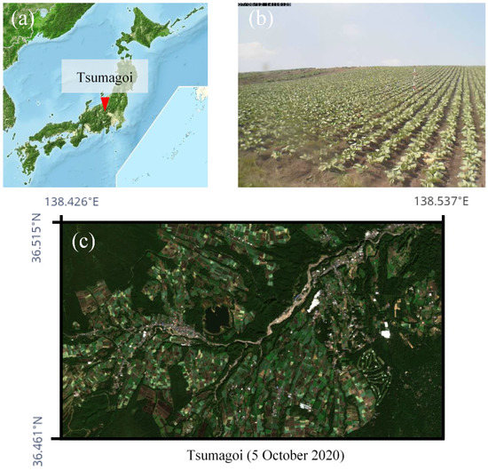
Figure 1.
Information about the study area. (a) Location of Tsumagoi. (b) A web-camera image of a cabbage field in Tsumagoi. (c) A 10-m resolution RGB image of the target area taken by Sentinel-2.
2.2. Data Acquisition
2.2.1. Sentinel Data
For this work, images of Sentinel-1A and Sentinel-2A were collected from the Copernicus Open Access Hub [34]. Revisit time of Sentinel-1A and Sentinel-2A are 6 and 5 days in Tsumagoi, since Tsumagoi is located in the mid-latitudes, while the observation frequency is approximately half in other regions. Only data from one equipment was used in this study to show efficiency of the proposed model also for other data limited regions.
Sentinel-1 data were acquired in interferometric wide swath (IW) mode, in the Ground Range Detected (GRD) format, which has 10-m spatial resolution. The SAR data processing includes: (1) Calibration (VH/VV polarization intensities to sigma naught), (2) single product speckle filtering by Lee Sigma filtering [35], (3) transformation of the backscatter coefficients (δ) to decibels (dB), and (4) Range-Doppler Terrain Correction using digital elevation model data. Preprocessing was conducted on Sentinel Platform (SNAP) Software [36]. Finally, the Sentinel-2 optical image was collocated with preprocessed Sentinel-1 data. In this work, the closest counterparts of SAR and optical data (acquired within 5 days) were extracted for collocation. Data were acquired from January 2019 to December 2020 for the study area shown in Figure 2. Less data was acquired during June to August, since summer is the rainy season for Tsumagoi. NDVI was calculated by Equation (1), using RED (4th band, 665-nm) and NIR (8th band, 842-nm) of the Sentinel-2 image.
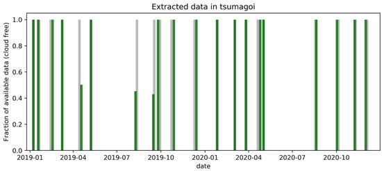
Figure 2.
Sentinel-1 and Sentinel-2 data acquired in Tsumagoi.
2.2.2. MODIS Data
In order to evaluate the applicability of the model to different satellite images, MODIS data were used. MOD09 and MYD09 (Terra and Aqua Surface Reflectance Daily L2G Global 250 m) products were acquired from EARTHDATA Search [37]. Cloudless Sentinel-2 and MODIS optical data which were acquired within 3 days were collocated for evaluation. The MODIS-data acquisition dates differed among the experiments; a detailed explanation is given in Section 4.2.1 and Section 4.3.1. NDVI was calculated by Equation (1), using RED (1st band, 620~670-nm) and NIR (2nd band, 841~876-nm) of the MODIS image.
3. Method
3.1. The CNN-Based Downscaling Model
Convolutional neural networks (CNN) have been successfully applied to many image processing problems, such as image classification [38], object recognition [39], and image generation [40]. Their main advantages are the capability to approximate complex non-linear end-to-end mappings including surrounding pixels and the parallel computational architecture. Recently, in the field of super-resolution, deep models with many parameters have been trained by using large datasets [19]. For super-resolution, manual labeling is not needed, because the reference data can be automatically generated from the data themselves. However, satellite data, especially in the cloudy region, are limited compared to general RGB images.
In this work, the architecture of the Super-Resolution Convolutional Neural Network (SRCNN) [41] was used, as shown in Figure 3 and Table 1. This model has fewer parameters [19] and is trainable with a smaller dataset. Models with similar architecture have also been used for NDVI estimation [27] and have shown acceptable results. Input and output are trimmed into a 1250-m (125 pixels in 10-m resolution) square patch with spacing of 400-m (40 pixels in 10-m resolution), referencing the aforementioned work [18]. By applying this trimming method to the target area (573 × 1016 pixels), 242 patches were extracted. No data augmentation was used in this study. The detailed information of input and output is summarized below.
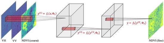
Figure 3.
Proposed C convolutional neural network (CNN) architecture for the downscaling of normalized difference vegetation index (NDVI).

Table 1.
Hyper-parameters of the proposed CNN. y(i) represents the variable in the equations of Figure 3.
- Input
- -
- VH: Sentinel-1, 10-m resolution
- -
- VV: Sentinel-1, 10-m resolution
- -
- NDVI: Sentinel-2 or MODIS (differs by experiment), 250-m resolution
- Output
- -
- NDVI Sentinel-2, 10 m
For inference, square patches for the test area were generated in the same way with 125 pixels of side length and 40 pixels of spacing. The output was then stitched into the original shape of the target area by taking the mean value for the overlapped region.
3.2. Concept of the Proposed Model
The model can be conceptually understood as downscaling using surrounding higher resolution SAR features. Figure 4 shows an example of an input and reference image patch pair. In the case of ×25 downscaling, one coarse NDVI pixel is an average (mixed-pixel) of 25 × 25 = 625 fine NDVI pixels. This is an ill-posed problem and cannot be solved exactly. CNN models have achieved considerable improvements, since they can consider surrounding pixels and the pattern of downscaling from images in the training set. Furthermore, by also considering SAR images, which have a strong relation with vegetation (as seen in Figure 4), the downscaled NDVI can be estimated with higher accuracy and using less data. SAR data can provide additional information related to surface roughness of target area. Since vegetation is mainly characterized by a vertical geometry, VV and VH components of SAR data can especially explain vegetation well [42]. For example, according to Figure 4, value of VH tend to become higher at area with vegetation (high NDVI values). This is due to the perturbation on vertical polarized signal emitted by the radar, since surface with vegetation tend to have rougher surface than the soil.
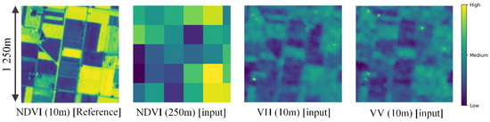
Figure 4.
A sample input and output patch pair: (First panel) 10-m NDVI from Sentinel-2; (second) 250-m NDVI by up-sampling 10-m Sentinel-2; (third) 10-m VH from Sentinel-1; (fourth) 10-m VV from Sentinel-1.
3.3. Training Settings
For loss function, L1-norm (Equation (2)) was selected after preliminary experiments. This result corresponds with the result for a similar task in [18].
For the optimization, Adam [43], which is one of the most widely used procedures, was adopted. In Adam, weights are updated by Equations (3)–(5), where m and v are the moving average of mean and uncentered variance, and g is the gradient on the current mini-batch. α and β are hyperparameters, and β was set to the following widely used and successful values: β1 = 0.9, and β2 = 0.999 [43].
In order to decide the number of epochs and the optimal α value for training, a preliminary experiment was conducted. To prevent data leakage, only data from 2019 were extracted for this experiment, since inference by the model was conducted using 2020 data in this study. Then, for the extracted data from 2019, one date was selected for the validation data and the model was trained by using data from other dates. For different α, this experiment was conducted for every acquired date in 2019, and the average training curve is shown in Figure 5. 250 epochs of training were sufficient for the convergence, and α = 0.001 performed the best after the convergence. In this work, the number of epochs was set to 250 and α was set to 0.001. Training was conducted on NVIDIA GPU, GeForce GTX 1080. The CNN model was implemented by using TensorFlow.
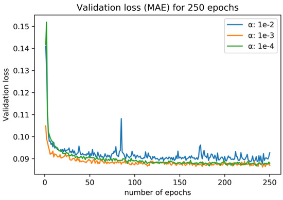
Figure 5.
Average loss and validation loss (L1-norm) for the preliminary training experiment. Different colors represent different α values.
4. Results
4.1. Model training with Sentinel-1 and Sentinel-2
4.1.1. Experimental Design
In this experiment, only Sentinel-2 data were used for NDVI: A pair of up-sampled 250-m Sentinel-2 NDVI and original 10-m Sentinel-2 NDVI were used for training. Up-sampling was calculated by averaging the 10-m resolution NDVI values within the 250-m grid. Data acquired during 2019 (1 January 2019~31 December 2019) was used for model training and data obtained in 2020 (1 January 2020~31 December 2020) were used for tests. For test data, only dates with 100% availability were selected for fair comparison. The prediction was evaluated using two metrics, the mean absolute error (MAE, Equation (2)) and Pearson’s correlation coefficient (ρ, Equation (6)). This validation was applied to all dates, and seasonal differences were discussed.
4.1.2. Results
In order to evaluate the proposed model, a linear regression model was used for baseline comparison. Input for the linear regression model corresponded with the input for the proposed model (VH, VV and 250-m NDVI), and is designed to learn the linear relationship between corresponding pixels.
Figure 6 shows the example of a qualitative result for Tsumagoi, 5 October 2020. The proposed CNN method (Figure 6f) is compared with linear regression (Figure 6c), the proposed model with only SAR data as input (Figure 6e, trained by SAR only), and only 250-m NDVI as input (Figure 6d, trained by NDVI only). Proposed method with both data generated a sharper image compared to other methods. Also, the linear regression seems to predict more precise features compared to input 250-m NDVI (Figure 6b) and proposed model with only NDVI input. This result implies that SAR data are effective for explaining NDVI features. On the other hand, proposed model with only SAR input captures fine features, but the difference in value is large compared to reference data (Figure 6a). This result implied that the SAR data and NDVI data works supportively for prediction, and each data supplies different information.
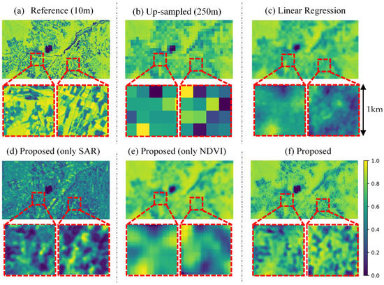
Figure 6.
Qualitative result in Tsumagoi, 5 October 2020. (a) 10-m Sentinel-2 NDVI. (b) Up-sampled Sentinel-2 NDVI (250-m), (c) Predicted NDVI by linear regression. (d) Predicted NDVI by the proposed model with only synthetic aperture radar (SAR) input. (e) Predicted NDVI by the proposed method with only NDVI input. (f) Predicted NDVI by the proposed method. The bottom row displays enlarged views of the area in the red square.
Quantitative results are shown in Table 2. The overall accuracy of proposed method is 0.090 in MAE and 0.734 in ρ. On average, the proposed model performed better than linear regression. Also, MAE and ρ of the linear regression appeared to have a strong positive relationship with the results of the proposed model.
Table 2.
Quantitative results for the target area. Dates are the acquisition dates for Sentinel-1. Interval days show the interval between the date of available imaginary from 2019 and the equivalent day in 2020. Calculated interval days including partly available data (images with clouds) are shown in parenthesis. Bold numbers represent best results for each date.
Seasonal differences are not clearly observed. However, interval days, which is the interval between the date of available imaginary from 2019 and the equivalent day in 2020, seemed to be related with accuracy. For data with a date interval of less than 7 days (3 March, 2 May, 4 December), the average MAE (0.081) was lower than the overall average and the average ρ (0.777) was higher than the overall average. On the other hand, for data with a date interval of more than 7 days (27 March, 20 April, 18 August, 5 October, 10 November), the average MAE (0.094) was higher than the overall average and the average ρ (0.723) was lower than the overall average.
Qualitative results show that the values of MAE and ρ do not necessarily have positive correlation. For example, the results for 18 August tend to have high MAE and high ρ. This can be explained by the difference in the NDVI histograms, as shown in Figure 7. From the NDVI images, the difference between fields is clearer on 18 August (high MAE, high ρ) than on 4 December (moderate MAE, moderate ρ). The bottom figure shows the histogram for distribution of NDVI. Histograms acquired in both dates have a distribution with two peaks. This is likely to be caused by the superposition of two NDVI distributions from different sources: Vegetation and background. In August, which is the mid-season for cropping, the NDVI differences are larger between fields, and the NDVI for the mountainous area is also large, which can also be observed from the expanded NDVI distribution shown in the histogram. For this expanded histogram, ρ and MAE tend to become larger. On the other hand, in December, the differences between fields in the original NDVI are smaller, which also causes the histogram of predicted NDVI to have a similar distribution. For this coherent distribution of NDVI, MAE tends to take a smaller value. The pros and cons of these different histograms tend to differ according to the application. For example, for evaluation of the NDVI value in a certain area, low MAE values may be better, while for classification of harvested and unharvested fields, high ρ may by better. However, more additional information can be obtained by downscaling for the seasons with latter histogram, since former information can be obtained from original 250-m resolution data.
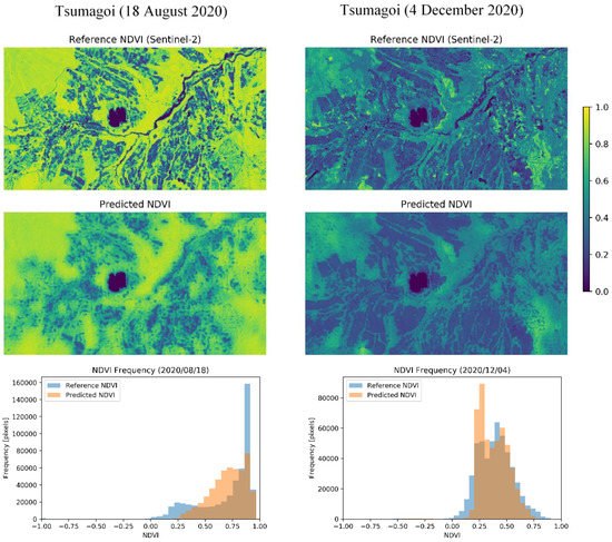
Figure 7.
Comparison between different seasons. For each date, the panels show (top) the original Sentinel-2 10-m NDVI, (middle) the predicted 10-m NDVI, and (bottom) the histogram of NDVI frequency.
According to the histograms in Figure 7, the model seems to make conservative predictions, especially for the data on 18 August. This can be improved by implementing different loss function or optimization methods for training. Also, using more data acquired during summer season for model training can be effective, since less summer data was acquired due to rainy season in Tsumagoi (see Figure 2).
4.2. Prediction with MODIS Data
In Section 4.1, the model was trained and evaluated with the pair of original Sentinel-2 10 m NDVI and up-sampled 250-m Sentinel-2 NDVI. However, in the case of practical application, this model needs to be applied not on up-sampled Sentinel-2 data but data from different satellite sources such as MODIS. In this section, the model trained by data from 2019 (see Section 4.1) was applied to 250-m NDVI from MODIS image to investigate its potential for application.
4.2.1. Data Information
Table 3 shows the date information for the acquired data. The corresponding MODIS data (see Section 2.2.2 for the detailed product information) were extracted according to the following protocol.
Table 3.
Date of acquired data. Hyphens (-) express no cloudless data available.
- -
- Search MODIS data within 3 days from the date of the Sentinel-2 data.
- -
- If cloudless data are not found within 3 days, no data are used
- -
- If any cloudless data is found from either Terra and Aqua, acquire all data for ensembling. (see Section 4.2.3 for a detailed explanation)
4.2.2. Experimental Design
In this section, the model trained in Section 4.1 (trained with the Sentinel-2 image pair, acquired in 2019) was adopted. The model predicted downscaled NDVI from the input of the MODIS 250-m NDVI and Sentinel-1 SAR image (the data pair shown in Table 3). Finally, the output image was evaluated by comparing it with the Sentinel-2 10-m NDVI acquired on a near date.
4.2.3. Difference between Sentinel-2 and MODIS NDVI
Mismatch in NDVI data acquired from different resolutions has been reported [44]. This was also the case for Sentinel-2 and MODIS, with the Sentinel-2 data appearing to show better correspondence with the field observation data [45]. This can be due to differences in data processing, acquisition time, and bandwidth difference.
In this research, the difference of NDVI between Sentinel-2 and MODIS was also measured. Table 4 shows the difference between acquired Sentinel-2 and MODIS NDVI. The columns “Terra” and “Aqua” show the original difference between MODIS and up-sampled Sentinel-2 data acquired in the same day. In previous research, time series filtering and anomaly detection was applied to daily MODIS NDVI data, and reported improved correspondence with Sentinel-2 NDVI data [45].
Table 4.
Average difference between acquired MODIS (Moderate Resolution Imaging Spectroradiometer) and Sentinel-2 NDVI for Tsumagoi. Sentinel-2 NDVI was up-sampled to 250-m for comparison. The date when both Terra and Aqua data were available was extracted for fair comparison.
In this study, in order to reduce the difference between MODIS and Sentinel-2 NDVI, median filtering was applied to NDVI acquired from Terra and Aqua before input as below:
- -
- Collect Terra and Aqua data within 3 days from Sentinel-2 data (see Section 4.2.1)
- -
- For all of the collected data, adopt the median value for each pixel as the ensembled value
The “Ensemble” column in Table 4 shows the difference between MODIS and Sentinel-2 NDVI after ensembling. Both MAE and ρ improved in average after ensembling. This may have been due to suppression of error with strong randomness.
4.2.4. Results
Quantitative results are shown in Table 5. On average, compared to the model with up-sampled Sentinel-2 input, MAE increased by 0.015, and ρ decreased by 0.085. Figure 8 shows the strong correlation in the MAE between input MODIS and up-sampled Sentinel-2 and in the increased MAE after prediction. This result implies room for improvement by suppressing the difference between MODIS NDVI and Sentinel-2 NDVI before input.
Table 5.
Comparison of prediction accuracy between Sentinel-2 input and MODIS input. The output is evaluated with original 10 m NDVI from Sentinel-2.
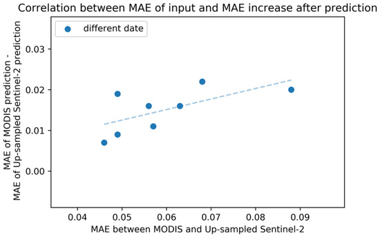
Figure 8.
Relation between MAE of input and MAE increase after MODIS prediction. X-axis shows MAE between input MODIS and up-sampled Sentinel-2 NDVI for each date. Y-axis represents (MAE of MODIS prediction) − (MAE of up-sampled Sentinel-2 NDVI prediction), both evaluated by the original 10-m Sentinel-2 NDVI.
Figure 9 shows the qualitative prediction results for Tsumagoi (5 October 2020). According to Table 5, the prediction results are moderate compared to the average in MAE and ρ. In Figure 9, the prediction by up-sampled Sentinel-2 NDVI (c) looks clearer compared to that by MODIS input (d), and the predicted values seem to be closer to the reference data, for example, near the lake area where the MAE between MODIS and Sentinel-2 was large before input (a). However, even for prediction with MODIS data, the prediction captures the characteristics of NDVI for fields to a certain extent.
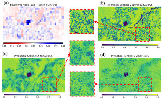
Figure 9.
Qualitative result for MODIS prediction in Tsumagoi (5 October 2020). (a) Error between MODIS and Sentinel-2 NDVI before input. (b) Reference 10-m NDVI from Sentinel-2. (c) Prediction with up-sampled 250-m Sentinel-2 NDVI as input. (d) Prediction with 250-m MODIS NDVI as input.
4.3. Example of an Application in Tsumagoi
The prediction with MODIS data was conducted and evaluated in Section 4.2. In this section, as a practical application, the proposed model is applied to 2020 data in Tsumagoi in order to enhance the temporal resolution of 10-m NDVI. As in the studies by [46,47], double cropping of cabbages takes place during the summer season in Tsumagoi. One goal of this application is to detect the timeline of double cropping by enhanced temporal and spatial resolution data.
4.3.1. Experimental Design
In this section, data acquired during 1 January 2019~31 December 2019 were used to train the proposed model (see Section 4.1). Then, the trained model was applied to MODIS data during 1 January 2020~31 December 2020 to predict the 10-m NDVI of the corresponding date. By combining these data with Sentinel-2 data collected in 1 January 2020~31 December 2020, NDVI data with both high spatial and high temporal resolution were generated. The data used for inference in this experiment are shown in Table 6.
Table 6.
Date information of the reference data.
4.3.2. Results
Figure 10 show images of Sentinel-2 NDVI and predicted NDVI by the proposed model during the growing season (5 May 2020~8 November 2020) in a time-line. For the predicted images, the input MODIS NDVI in 250-m resolution are shown in the left column. Predicted images reflect the distribution of NDVI in the input MODIS image and show change in NDVI values by seasonal change. Predicted image in 19 June seems to have excess NDVI considering images before and after. However, this can be also observed in the MODIS input of corresponding day.
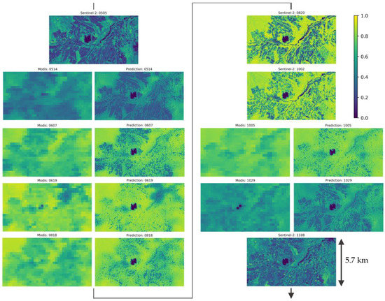
Figure 10.
Sentinel-2 and predicted NDVI during the growing season (5 May 2020~8 November 2020). Type and date of images are shown in the title of each image. For each date of predicted NDVI, input 250-m NDVI are shown in the left column and predicted NDVI are shown in the right column.
Results of time series plot are shown in Figure 11. Three locations with different land usages were selected for time-series evaluation. Location A is a crop field with single cropping, location B is a fallow land, and location C is a crop field with double cropping, which was confirmed by Sentinel-2 images. The mean value within 3 × 3 (30 m × 30 m) center pixels of each location is used as the extracted NDVI value. The three plots in Figure 11 shows the transition of NDVI value for each location. Blue plots indicate the values extracted from MODIS data (250-m resolution, cloudless images were extracted), and red plot shows 10-m resolution NDVI with combination of Sentinel-2 and prediction by the proposed model using MODIS and Sentinel-1 data. Among the red plots, outlined plots represent estimation from the proposed model and the error bar represents the average MAE (see Section 4.2.4).
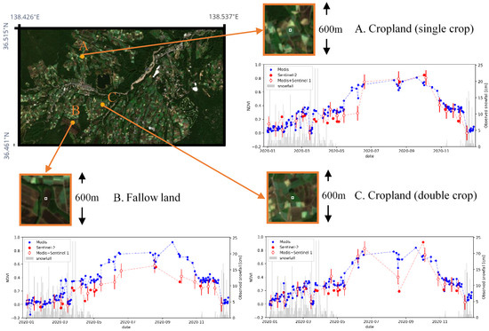
Figure 11.
Time series plot of NDVI by original MODIS data and the combination of Sentinel-2 and MODIS+Sentinel-1 prediction. Image in upper-left shows view of the Tsumagoi area in 5 October 2020 acquired from Sentinel-2. Three points with different land usages were extracted. Three panels with orange frames shows zoomed image for the selected locations. The average value of the center 3 × 3 pixels, shown in white square inside each panel, is used as the estimated NDVI. The plot shows the transition of NDVI values. Blue plots represent the MODIS 250-m NDVI data and red plots show 10-m NDVI from the combination of Sentinel-2 NDVI and estimated NDVI from MODIS and Sentinel-1 by the proposed model. Outlined red plots represent estimation from the proposed model with error bars representing average MAE values evaluated in Section 4.2.4. Gray bars show the amount of snowfall observed at Kusatsu Observatory.
In location A (single crop), the 250-m resolution plot (blue) has increase of NDVI in May, which is earlier compared to that in the 10-m resolution plot (red). In the resolution of 250-m, one pixel becomes a mixed pixel and includes NDVI values of surrounding fields. In such resolution, the planting season cannot be estimated accurately, considering that planting is conducted earlier in crop-fields with double cropping compared to single cropping fields in order to run two growing cycles. By downscaling to 10-m resolution, planting season can be estimated clearer by decomposing the mixed-pixel.
In location B (fallow land), transition of NDVI in 250-m resolution is higher compared to that in 10-m resolution. This is because the value in 250 m resolution becomes the average of surrounding pixels, which has higher NDVI values.
In location C (double crop), 10-m resolution NDVI plot shows an increase from May to June, but the NDVI drops in August, and then rise again in September. This is likely to be the result of double cropping, since the field camera survey conducted in previous researches also observed the first harvest at the end of July [46,47]. The drop of NDVI values can be seen clearer in 10-m resolution. However, the downscaled data still seems to have a larger value at the end of August compared to the reference Sentinel-2 data. This implies that the model is generating conservative predictions that are closer to the average value. The modification of loss function or the architecture of Generative Adversarial Networks (GANs) could be applied to predict sharper values in a future study [48,49].
A decrease in NDVI can be observed at all locations in March and December. The observed snowfall data was acquired from the Japan Meteorological Agency. The amount of snowfall observed at Kusatsu Observatory (15 km away from the target area but with similar meteorological conditions), is shown by the bar graph in Figure 11. The decrease in NDVI is likely to be caused by snowfall, since intense snowfall can be observed around the date of the decreased NDVI.
The Sentinel-2 observed NDVI and predicted NDVI at the near date have close values in average. Time series anomaly detection or filtering can be applied to further increase the accuracy. Also, applications such as land cover classification can be improved by using high temporal and spatial resolution image generated by the proposed method.
Figure 12 shows a comparison between the time series plot made by the original 250-m resolution MODIS NDVI, Sentinel-2 10-m NDVI, and the combination of Sentinel-2 and downscaled NDVI, applied to adjacent crop fields. Time series plot by MODIS NDVI (Figure 12a) has sufficient temporal resolution to track the vegetation transition, but difference between the two fields are unclear due to insufficient spatial resolution. Difference between the two fields can be observed in the time series plot by Sentinel-2 NDVI (Figure 12b), but cannot track the transition of vegetation enough due to insufficient temporal resolution. The NDVI of the two fields are sometimes in the same 250-m resolution pixel with same values, and even if not, they have similar values due to mixed pixel, where 1 pixel becomes the average of the surrounding 250 m × 250 m. By combining Sentinel-2 NDVI with predicted 10-m resolution NDVI (Figure 12c), both high spatial resolution to distinguish the difference between the two fields and high temporal resolution to track the transition of vegetation growth can be achieved. By applying this method, double cropping in field A and single cropping in field B could be observed.
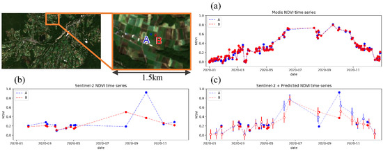
Figure 12.
Comparison of NDVI time series plot for adjacent crop fields. (left-top) Location of the target crop fields. Color of the plots represent each field. (a) Plot by cloudless MODIS 250-m data. (b) Plot by Sentinel-2 10-m data. (c) Plot by combination of Sentinel-2 and estimation from the proposed model. Outlined plot represent estimation from the proposed model and error bar shows average MAE (see Section 4.2.4).
5. Discussion
5.1. Pros and Cons
In recent years, several researches have focused on the coordination of optical and SAR images. One popular approach is to use SAR, which is available for cloudy days, to estimate the optical features under cloudy conditions. However, a model trained in this manner will rely fully on SAR for its prediction, causing it to be unstable against SAR noise or observation error. This will worsen the ability of the model to make predictions using data acquired from different observations or dates.
In the proposed model, 250-m resolution NDVI was input into the model with SAR, which would lead to less dependence on SAR data, assuming that the input NDVI is the up-sampled image of the actual NDVI. This can lead to stable prediction for different locations and seasons, which is also not ideal.
However, there are still sources of error for the prediction. One is the difference between MODIS and Sentinel-2 NDVI. This can be suppressed to a certain extent by median ensembling of Terra and Aqua NDVI (see Section 4.2.3). In addition, temporal anomaly filtering or smoothing can also be applied to reduce difference between MODIS and Sentinel-2 NDVI furthermore [45]. A second source of error was the data included in the training set. The quantity and quality of data necessary for precise prediction can vary according to the features of the target area: In general, an area with high variation of land cover will require more and more variable training data. However, for locations that experience rainy and dry seasons, the available optical data will be scarce for the rainy season, even though dynamic change in cropland usually takes place during the rainy season. This mismatch between training data and prediction demand should be considered. One way to overcome this issue is by data augmentation [50]. Applying data augmentation to scarce data in the rainy season can be effective. Another possible solution is fine-tuning, which has also been successfully applied to SAR images [51]. Applying a model pre-trained with data under similar condition can enhance accuracy with a small training dataset.
5.2. Effective Condition for Application
After applying the proposed model to different seasons and locations, it can be concluded that there are two important characteristics when choosing an ideal location for the application. One is the histogram of NDVI, as discussed above in Section 4.1.2. Ideal shape for the histogram may differ by application. However, in order to exploit the benefits of enhanced spatial resolution, a high ρ value is preferable (see Section 4.3.2), which is likely to be derived from an area of land with an expanded NDVI histogram. The second important characteristic is the ability to explain differences in land cover by VH and VV backscatter within the target area. If the soil and crop area have the same or similar backscatter characteristics, predicting the difference would also be difficult for the model. Also, transition of backscatter values differs by crop types [16]. This availability to analyze the land-cover differences by backscatter values can be preliminarily confirmed by applying a heuristic linear regression model in the target area, since the results of linear regression and the proposed model was strongly correlated (see Section 4.1.2), which may be a simple indicator of the explainability of NDVI from backscatter signals. In addition, unsupervised learning can be applied in this area to confirm the difference of backscatter signals between different landcover types.
6. Conclusions
This study proposed a method to downscale the spatial resolution of NDVI from 250-m MODIS resolution to 10-m Sentinel-2 resolution. The proposed model used 10-m resolution SAR with 250-m resolution NDVI as input to learn the concept of downscaling. The proposed model was first trained with a Sentinel-2 NDVI pair (an original 10-m image and an up-sampled 250-m image) acquired in 2019. The experimental results showed that the prediction was reasonably accurate (MAE = 0.090, ρ = 0.734 on average for the test data acquired in 2020). Then, the trained model was applied to downscale NDVI from MODIS NDVI data in Tsumagoi. Even with the difference between MODIS NDVI and Sentinel-2 NDVI, the accuracy of downscaled NDVI was acceptable (MAE = 0.108, ρ = 0.650 on average). Finally, the model was applied to enhance the temporal resolution (approximately × 2.5 data) of NDVI with high spatial resolution (10 m), and it successfully observed the features of a double cropping of cabbage in Tsumagoi.
However, a method to reduce the difference between the original MODIS NDVI and Sentinel-2 NDVI will be needed for further improvement. A method for locating effective locations for the application is also needed. In summary, this study provides a new approach to produce 10-m resolution NDVI data with acceptable accuracy when cloudless MODIS NDVI and Sentinel-1 SAR data is available. This can be a step for improving both the temporal and the spatial resolution in vegetation monitoring, and is hoped to contribute to the improvement of food security and production.
Author Contributions
Conceptualization, R.N. and K.O.; methodology, R.N.; analysis, R.N; writing, R.N; supervision, K.O. All authors have read and agreed to the published version of the manuscript.
Funding
This research was funded by The Foundation for the Promotion of Industrial Science (FPIS).
Conflicts of Interest
The authors declare no conflict of interest.
References
- Grafton, R.Q.; Daugbjerg, C.; Qureshi, M.E. Towards food security by 2050. Food Secur. 2015, 7, 179–183. [Google Scholar] [CrossRef]
- Farooq, M.S.; Riaz, S.; Abid, A.; Umer, T.; Bin Zikria, Y. Role of IoT Technology in Agriculture: A Systematic Literature Review. Electronics 2020, 9, 319. [Google Scholar] [CrossRef]
- Tsouros, D.C.; Bibi, S.; Sarigiannidis, P.G. A review on UAV-based applications for precision agriculture. Information 2019, 10, 349. [Google Scholar] [CrossRef]
- Usha, K.; Singh, B. Potential applications of remote sensing in horticulture—A review. Sci. Hortic. 2013, 153, 71–83. [Google Scholar] [CrossRef]
- Yang, C.; Everitt, J.H.; Murden, D. Evaluating high resolution SPOT 5 satellite imagery for crop identification. Comput. Electron. Agric. 2011, 75, 347–354. [Google Scholar] [CrossRef]
- Dong, J.; Xiao, X.; Kou, W.; Qin, Y.; Zhang, G.; Li, L.; Jin, C.; Zhou, Y.; Wang, J.; Biradar, C.; et al. Tracking the dynamics of paddy rice planting area in 1986–2010 through time series Landsat images and phenology-based algorithms. Remote Sens. Environ. 2015, 160, 99–113. [Google Scholar] [CrossRef]
- Inglada, J.; Arias, M.; Tardy, B.; Hagolle, O.; Valero, S.; Morin, D.; Dedieu, G.; Sepulcre, G.; Bontemps, S.; Defourny, P.; et al. Assessment of an Operational System for Crop Type Map Production Using High Temporal and Spatial Resolution Satellite Optical Imagery. Remote Sens. 2015, 7, 12356–12379. [Google Scholar] [CrossRef]
- Zhang, C.; Li, W.; Travis, D. Gaps-fill of SLC-off Landsat ETM+ satellite image using a geostatistical approach. Int. J. Remote Sens. 2007, 28, 5103–5122. [Google Scholar] [CrossRef]
- Zeng, C.; Shen, H.; Zhang, L. Recovering missing pixels for Landsat ETM+ SLC-off imagery using multi-temporal regression analysis and a regularization method. Remote Sens. Environ. 2013, 131, 182–194. [Google Scholar] [CrossRef]
- Zhang, X.; Qin, F.; Qin, Y. Study on the Thick Cloud Removal Method Based on Multi-Temporal Remote Sensing Images. In Proceedings of the 2010 International Conference on Multimedia Technology, Ningbo, China, 2–4 October 2010; pp. 1–3. [Google Scholar]
- Julien, Y.; Sobrino, J.A. Comparison of cloud-reconstruction methods for time series of composite NDVI data. Remote Sens. Environ. 2010, 114, 618–625. [Google Scholar] [CrossRef]
- Lu, X.; Liu, R.; Liu, J.; Liang, S. Removal of Noise by Wavelet Method to Generate High Quality Temporal Data of Terrestrial MODIS Products. Photogramm. Eng. Remote Sens. 2007, 73, 1129–1139. [Google Scholar] [CrossRef]
- Waske, B.; Braun, M. Classifier ensembles for land cover mapping using multitemporal SAR imagery. ISPRS J. Photogramm. Remote Sens. 2009, 64, 450–457. [Google Scholar] [CrossRef]
- Chapman, B.; McDonald, K.; Shimada, M.; Rosenqvist, A.; Schroeder, R.; Hess, L. Mapping Regional Inundation with Spaceborne L-Band SAR. Remote Sens. 2015, 7, 5440–5470. [Google Scholar] [CrossRef]
- Kurosu, T.; Fujita, M.; Chiba, K. Monitoring of rice crop growth from space using the ERS-1 C-band SAR. IEEE Trans. Geosci. Remote Sens. 1995, 33, 1092–1096. [Google Scholar] [CrossRef]
- Bazzi, H.; Baghdadi, N.; El Hajj, M.; Zribi, M.; Minh, D.H.T.; Ndikumana, E.; Courault, D.; Belhouchette, H. Mapping Paddy Rice Using Sentinel-1 SAR Time Series in Camargue, France. Remote Sens. 2019, 11, 887. [Google Scholar] [CrossRef]
- Zhao, W.; Qu, Y.; Chen, J.; Yuan, Z. Deeply synergistic optical and SAR time series for crop dynamic monitoring. Remote Sens. Environ. 2020, 247, 111952. [Google Scholar] [CrossRef]
- Scarpa, G.; Gargiulo, M.; Mazza, A.; Gaetano, R. A CNN-Based Fusion Method for Feature Extraction from Sentinel Data. Remote Sens. 2018, 10, 236. [Google Scholar] [CrossRef]
- Anwar, S.; Khan, S.; Barnes, N. A Deep Journey into Super-resolution: A survey. arXiv 2020, arXiv:1904.07523. [Google Scholar] [CrossRef]
- Lin, C.-H.; Bioucas-Dias, J.M. An Explicit and Scene-Adapted Definition of Convex Self-Similarity Prior With Application to Unsupervised Sentinel-2 Super-Resolution. IEEE Trans. Geosci. Remote Sens. 2020, 58, 3352–3365. [Google Scholar] [CrossRef]
- Lanaras, C.; Bioucas-Dias, J.; Galliani, S.; Baltsavias, E.; Schindler, K. Super-resolution of Sentinel-2 images: Learning a globally applicable deep neural network. ISPRS J. Photogramm. Remote Sens. 2018, 146, 305–319. [Google Scholar] [CrossRef]
- Yokoya, N. Texture-Guided Multisensor Superresolution for Remotely Sensed Images. Remote Sens. 2017, 9, 316. [Google Scholar] [CrossRef]
- Gao, F.; Masek, J.; Schwaller, M.; Hall, F. On the blending of the Landsat and MODIS surface reflectance: Predicting daily Landsat surface reflectance. IEEE Trans. Geosci. Remote Sens. 2006, 44, 2207–2218. [Google Scholar] [CrossRef]
- Li, J.; Wang, S.; Gunn, G.; Joosse, P.; Russell, H.A. A model for downscaling SMOS soil moisture using Sentinel-1 SAR data. Int. J. Appl. Earth Obs. Geoinform. 2018, 72, 109–121. [Google Scholar] [CrossRef]
- Amazirh, A.; Merlin, O.; Er-Raki, S. Including Sentinel-1 radar data to improve the disaggregation of MODIS land surface temperature data. ISPRS J. Photogramm. Remote Sens. 2019, 150, 11–26. [Google Scholar] [CrossRef]
- Bai, J.; Cui, Q.; Zhang, W.; Meng, L. An Approach for Downscaling SMAP Soil Moisture by Combining Sentinel-1 SAR and MODIS Data. Remote Sens. 2019, 11, 2736. [Google Scholar] [CrossRef]
- Mazza, A.; Gargiulo, M.; Scarpa, G.; Gaetano, R. Estimating the NDVI from SAR by Convolutional Neural Networks. In Proceedings of the IGARSS 2018—2018 IEEE International Geoscience and Remote Sensing Symposium, Valencia, Spain, 23–27 July 2018; pp. 1954–1957. [Google Scholar]
- Veloso, A.; Mermoz, S.; Bouvet, A.; Le Toan, T.; Planells, M.; Dejoux, J.-F.; Ceschia, E. Understanding the temporal behavior of crops using Sentinel-1 and Sentinel-2-like data for agricultural applications. Remote Sens. Environ. 2017, 199, 415–426. [Google Scholar] [CrossRef]
- Bousbih, S.; Zribi, M.; Lili-Chabaane, Z.; Baghdadi, N.; El Hajj, M.; Gao, Q.; Mougenot, B. Potential of Sentinel-1 Radar Data for the Assessment of Soil and Cereal Cover Parameters. Sensors 2017, 17, 2617. [Google Scholar] [CrossRef] [PubMed]
- Mattia, F.; Le Toan, T.; Picard, G.; Posa, F.I.; D’Alessio, A.; Notarnicola, C.; Gatti, A.M.; Rinaldi, M.; Satalino, G.; Pasquariello, G. Multitemporal c-band radar measurements on wheat fields. IEEE Trans. Geosci. Remote Sens. 2003, 41, 1551–1560. [Google Scholar] [CrossRef]
- Benedetti, R.; Rossini, P. On the use of NDVI profiles as a tool for agricultural statistics: The case study of wheat yield estimate and forecast in Emilia Romagna. Remote Sens. Environ. 1993, 45, 311–326. [Google Scholar] [CrossRef]
- Lunetta, R.S.; Knight, J.F.; Ediriwickrema, J.; Lyon, J.G.; Worthy, L.D. Land-cover change detection using multi-temporal MODIS NDVI data. Remote Sens. Environ. 2006, 105, 142–154. [Google Scholar] [CrossRef]
- Yang, L.; Wylie, B.K.; Tieszen, L.L.; Reed, B.C. An Analysis of Relationships among Climate Forcing and Time-Integrated NDVI of Grasslands over the U.S. Northern and Central Great Plains. Remote Sens. Environ. 1998, 65, 25–37. [Google Scholar] [CrossRef]
- ESA. Copernicus Sentinel Data 2019~2020, Processed by ESA. Available online: https://scihub.copernicus.eu/ (accessed on 24 December 2020).
- Lee, J.-S.; Wen, J.-H.; Ainsworth, T.L.; Chen, K.-S.; Chen, A.J. Improved Sigma Filter for Speckle Filtering of SAR Imagery. IEEE Trans. Geosci. Remote Sens. 2009, 47, 202–213. [Google Scholar] [CrossRef]
- ESA. SNAP (Sentinel Application Platform) Software. Available online: https://step.esa.int/main/toolboxes/snap/ (accessed on 6 December 2020).
- Vermote, E.F.; El Saleous, N.Z.; O Justice, C. Atmospheric correction of MODIS data in the visible to middle infrared: First results. Remote Sens. Environ. 2002, 83, 97–111. [Google Scholar] [CrossRef]
- Krizhevsky, A.; Sutskever, I.; Hinton, G.E. Imagenet classification with deep convolutional neural networks. Commun. ACM 2017, 60, 84–90. [Google Scholar] [CrossRef]
- He, K.; Gkioxari, G.; Dollár, P.; Girshick, R. Mask R-CNN. arXiv 2018, arXiv:1703.06870. [Google Scholar]
- Zhu, J.-Y.; Park, T.; Isola, P.; Efros, A.A. Unpaired Image-to-Image Translation Using Cycle-Consistent Adversarial Networks. arXiv 2020, arXiv:1703.10593. [Google Scholar]
- Dong, C.; Loy, C.C.; He, K.; Tang, X. Image Super-Resolution Using Deep Convolutional Networks. IEEE Trans. Pattern Anal. Mach. Intell. 2015, 38, 295–307. [Google Scholar] [CrossRef] [PubMed]
- Wu, S.-T.; Sader, S. Multipolarization SAR Data for Surface Feature Delineation and Forest Vegetation Characterization. IEEE Trans. Geosci. Remote Sens. 1987, 25, 67–76. [Google Scholar] [CrossRef]
- Kingma, D.P.; Ba, J. Adam: A method for stochastic optimization. arXiv 2017, arXiv:1412.6980. [Google Scholar]
- Ryu, J.-H.; Na, S.-I.; Cho, J. Inter-Comparison of Normalized Difference Vegetation Index Measured from Different Footprint Sizes in Cropland. Remote Sens. 2020, 12, 2980. [Google Scholar] [CrossRef]
- Lange, M.; DeChant, B.; Rebmann, C.; Vohland, M.; Cuntz, M.; Doktor, D. Validating MODIS and Sentinel-2 NDVI Products at a Temperate Deciduous Forest Site Using Two Independent Ground-Based Sensors. Sensors 2017, 17, 1855. [Google Scholar] [CrossRef] [PubMed]
- Oki, K.; Mitsuishi, S.; Ito, T.; Mizoguchi, M. An Agricultural Monitoring System Based on the Use of Remotely Sensed Imagery and Field Server Web Camera Data. GISci. Remote Sens. 2009, 46, 305–314. [Google Scholar] [CrossRef]
- Oki, K.; Mizoguchi, M.; Noborio, K.; Yoshida, K.; Osawa, K.; Mitsuishi, S.; Ito, T. Accuracy comparison of cabbage coverage estimated from remotely sensed imagery using an unmixing method. Comput. Electron. Agric. 2011, 79, 30–35. [Google Scholar] [CrossRef]
- Reyes, M.F.; Auer, S.; Merkle, N.; Henry, C.; Schmitt, M. SAR-to-Optical Image Translation Based on Conditional Generative Adversarial Networks—Optimization, Opportunities and Limits. Remote Sens. 2019, 11, 2067. [Google Scholar] [CrossRef]
- Wang, L.; Xu, X.; Yu, Y.; Yang, R.; Gui, R.; Xu, Z.; Pu, F. SAR-to-Optical Image Translation Using Supervised Cycle-Consistent Adversarial Networks. IEEE Access 2019, 7, 129136–129149. [Google Scholar] [CrossRef]
- Perez, L.; Wang, J. The Effectiveness of Data Augmentation in Image Classification using Deep Learning. arXiv 2017, arXiv:1712.04621. [Google Scholar]
- Wang, Y.; Wang, C.; Zhang, H. Ship Classification in High-Resolution SAR Images Using Deep Learning of Small Datasets. Sensors 2018, 18, 2929. [Google Scholar] [CrossRef]


Publisher’s Note: MDPI stays neutral with regard to jurisdictional claims in published maps and institutional affiliations. |
© 2021 by the authors. Licensee MDPI, Basel, Switzerland. This article is an open access article distributed under the terms and conditions of the Creative Commons Attribution (CC BY) license (http://creativecommons.org/licenses/by/4.0/).