Abstract
Over semi-arid agricultural areas, the surface energy balance and its components are largely dependent on the soil water availability. In such conditions, the land surface temperature (LST) retrieved from the thermal bands has been commonly used to represent the high spatial variability of the surface evaporative fraction and associated fluxes. In contrast, however, the soil moisture (SM) retrieved from microwave data has rarely been used thus far due to the unavailability of high-resolution (field scale) SM products until recent times. Soil evaporation is controlled by the surface SM. Moreover, the surface SM dynamics is temporally related to root zone SM, which provides information about the water status of plants. The aim of this work was to assess the gain in terms of flux estimates when integrating microwave-derived SM data in a thermal-based energy balance model at the field scale. In this study, SM products were derived from three different methodologies: the first approach inverts SM, labeled hereafter as ‘SMO20’, from the backscattering coefficient and the interferometric coherence derived from Sentinel-1 products in the water cloud model (WCM); the second approach inverts SM from Sentinel-1 and Sentinel-2 data based on machine learning algorithms trained on a synthetic dataset simulated by the WCM noted ‘SME16’; and the third approach disaggregates the soil moisture active and passive SM at 100 m resolution using Landsat optical/thermal data ‘SMO19’. These SM products, combined with the Landsat based vegetation index and LST, are integrated simultaneously within an energy balance model (TSEB-SM) to predict the latent (LE) and sensible (H) heat fluxes over two irrigated and rainfed wheat crop sites located in the Haouz Plain in the center of Morocco. H and LE were measured over each site using an eddy covariance system and their values were used to evaluate the potential of TSEB-SM against the classical two source energy balance (TSEB) model solely based on optical/thermal data. Globally, TSEB systematically overestimates LE (mean bias of 100 W/m2) and underestimates H (mean bias of −110 W/m2), while TSEB-SM significantly reduces those biases, regardless of the SM product used as input. This is linked to the parameterization of the Priestley Taylor coefficient, which is set to αPT = 1.26 by default in TSEB and adjusted across the season in TSEB-SM. The best performance of TSEB-SM was obtained over the irrigated field using the three retrieved SM products with a mean R2 of 0.72 and 0.92, and a mean RMSE of 31 and 36 W/m2 for LE and H, respectively. This opens up perspectives for applying the TSEB-SM model over extended irrigated agricultural areas to better predict the crop water needs at the field scale.
1. Introduction
Mapping evapotranspiration (ET) is of paramount importance in water resources management [1] as it is the most important component that controls the energy and water balance [2]. In addition, an accurate ET estimate at a large scale is imperative, especially over arid and semi-arid areas where the vegetation cover is heterogeneous and where plants are subject to stress and water shortages due to limited soil water availability. Therefore, a spatialized estimation of ET can help manage the overall water resources in a sustainable manner. Over extended areas, remote sensing is the only viable technique that can provide spatially explicit ET using energy balance methods and has shown great potential for characterizing land surfaces through land use, vegetation coverage, water stress, etc. Amongst the variety of remotely sensed land-surface variables, three are particularly pertinent to ET estimation: vegetation cover index, land surface temperature (LST), and surface soil moisture (SM).
The normalized difference vegetation index (NDVI) is one of the most commonly used vegetation index to feed ET models [3]. It is computed from red and near infrared bands and can be considered as a useful indicator to characterize vegetation status, and consequently ET rates [4]. NDVI is classically used to derive the vegetation fraction cover (fc), which helps constrain the partition between soil evaporation and plant transpiration [5]. LST is a signature of the energy balance as well as mainly controlled by the soil water availability, especially in arid and semi-arid areas. In recent decades, many efforts have been devoted to extract spatially distributed LST data from remotely sensed thermal infrared data. Nowadays, many optical/thermal sensors on board satellites provide images of NDVI and LST at high spatial resolution ranging from 30 to 100 m for applications in monitoring the Earth’s surface processes [6].
At the same time, SM plays a key role in the evaporation process and is considered as an essential component in meteorological and hydrological forecasting [7]. Microwave remote sensing is recognized as the most promising and powerful tool for deriving large scale SM products because microwaves are not affected by atmospheric conditions and at low frequencies, measurements are strongly related to the water content in the first few centimeters of the soil [8]. SM is currently derived at a global scale from microwave radiometer data such as AMSR-E (Advanced Microwave Scanning Radiometer-EOS, [9]) at the C band (4–8 GHz) and SMOS (Soil Moisture and Ocean Salinity, [10]) or SMAP (Soil Moisture Active and Passive, [11]) at the L band (1.4 GHz). One drawback is that passive microwave radiometry provides coarse spatial resolution data (i.e., several tenths of kilometers). This coarse spatial resolution is therefore unsuitable for many applications such as irrigation management and identifying crop stress at a field scale, particularly over heterogeneous surfaces. The SMAP mission [11] was expected to provide SM at a spatial resolution of 9 km at three days repeat intervals by combining radar and radiometer measurements. However, the radar on broad SMAP stopped transmitting on July 2015 due to an anomaly that involved the radar’s high-power amplifier, and since then, SMAP has continued to work with data from the radiometer only.
As agricultural applications need remotely sensed SM at high spatial and temporal resolutions, therefore, great progress has been made to improve the spatial resolution of readily available SM data. A review of different methodologies for disaggregating passive microwave data for high resolution SM has recently been reported by Sabaghy et al. (2018) [12] and Peng et al. (2017) [13]. Santi et al. (2010) [14] downscaled the Advanced Microwave Remote Scanning Radiometer Earth Observing System (AMSR-E) at 10 km using the radiometer-based smoothing filter-based intensity modulation (SFIM) model. Gevaert et al. (2015) [15] used brightness temperatures sharpened by the SFIM technique and the Land Parameter Retrieval Model (LPRM, [16]) to retrieve soil moisture at 10 km from AMSR-E. Along the same line, Chan et al. 2018 [17] disaggregated the SMAP brightness temperature to 9 km using an interpolation technique, resulting in soil moisture estimates at a 9 km resolution. Other methodologies have been exploited such as the combination of passive microwave and optical/thermal data within a disaggregation algorithm to estimate SM at a 1 km resolution [18,19] or 100 m resolution [20]; the combination of passive microwave and in-situ measurements within a high resolution land data assimilation system (HRLDAS) to predict SM at 1 km resolution [21]; the combination of passive and active microwave data to estimate SM at a 100 m–3 km resolution [21,22,23]; and using the machine learning algorithm to disaggregate coarse-scale remotely sensed SM from 10 to 1 km resolution using high resolution auxiliary data [24]. The point is that all these approaches have limitations and uncertainties due to specific sensitivities to surface and atmospheric conditions [13,25].
Alternatively, C-band SAR (synthetic aperture radar) observations such as those collected by the recently launched Sentinel-1 can provide SM at 20 m resolution every six days [26]. Over covered soils, the C-band Sentinel-1 is affected by soil roughness and vegetation characteristics, and the backscattering coefficient σ0 has shown its strong sensitivity to SM, soil roughness, and vegetation characteristics [27,28,29,30]. Therefore, several models and approaches have been developed to retrieve SM. The most commonly used backscattering model is the semi-empirical water cloud model (WCM) [31]. Coupled to a soil backscatter model, WCM estimates the total signal as the incoherent sum of vegetation, soil and the soil attenuated by the vegetation cover contributions. The widespread use of this model originates not only from the good results obtained, but also from its simplicity. Unlike more complex models, WCM only needs one or two variables to describe the vegetation in the model. Theoretically, it is the vegetation water content [31]. However, the recent research has focused mainly on variables derived from remotely sensed data. Generally, the variables are derived from optical observations such as the plant height [32], leaf area index (LAI) [33,34], and NDVI [29,34,35]. Recently, Ouaadi et al. (2020) [30] developed a new approach to invert SM over wheat crops based on the use of Sentinel-1 data only (the interferometric coherence and backscatter coefficient), without the need of any ancillary data. The interferometric coherence was used to describe the vegetation contribution in the WCM and made it possible to get away from the dependence on optical data, which are restricted by weather and illumination conditions.
Several ET modeling approaches have been reported in the literature. At large scale, the surface energy balance (SEB) models forced by LST data represent a good trade-off between accuracy and operationality over complex landscapes. The TSEB (two source energy balance, [36]) model is one of the commonly used SEB models, and has been widely used over several fields with contrasted conditions [37,38,39,40]. However, various modifications have been applied in the model to improve its accuracy in terms of H/LE estimates [41,42]. In the same way, Ait Hssaine et al. (2018) [43] used surface SM data as an additional constraint on the TSEB model (named the TSEB-SM model) and calibrated the soil evaporation and plant transpiration separately to predict an accurate total ET. TSEB-SM has shown its robustness regarding ET estimates as it adjusts the Priestley Taylor coefficient according to the actual soil water availability (accounting for crop water stress regardless of the soil evaporation rate) and to the actual vegetation water status (hence representing the senescence period). TSEB-SM was also tested using remotely sensed data using SMOS SM disaggregated to a 1 km resolution and the Moderate resolution Imaging Spectroradiometer (MODIS) LST/NDVI data over a rainfed wheat, indicating coherent results [44]. However, one major shortcoming of this previous approach is that it operates at a 1 km resolution, which is very coarse for agricultural applications.
Over heterogenous sites with typical parcel size of tens to hundreds of meters, it is therefore of crucial importance to develop new methodologies to capture the ET dynamics at high-spatial resolution. In this context, the present work builds on the recent advances of high-resolution SM products to assess the utility of SM information to represent the surface energy balance over the highly heterogeneous landscape of semi-arid agricultural areas. In particular, this study aims to quantify the gain in terms of flux accuracy when integrating SM to the classic TSEB model based only on LST/NDVI data. In practice, different SM products at high-resolution with different degrees of complexity (derived from Sentinel-1 or from the disaggregation of SMAP data), in addition to LST/NDVI data were integrated within TSEB-SM to predict latent and sensible heat fluxes over two wheat crop sites in an irrigated and rainfed area of central Morocco where eddy covariance measurements were collected.
2. Data Description and Method
2.1. Study Area
The study was carried out at two sites in the Tensift Basin in central Morocco during the 2017–2018 agricultural season. The first site is a rainfed wheat field located about 40 km east of Marrakech (“Sidi Rahal”), while the second is an irrigated wheat field located approximately 70 km west of Marrakech (“Chichaoua”) (Figure 1). The climate in the Tensift region is semi-arid. Rainfall is low and irregular, generally occurring in a single wet season from November to April. The mean annual rainfall is about 250 mm/year while the reference evapotranspiration ET0 is about 1600 mm/year [45,46].
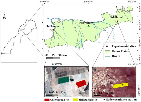
Figure 1.
Location of the two study sites, the rainfed wheat crop in the Sidi Rahal area (East of Marrakech) and the drip-irrigated wheat crop in the Chichaoua site (West of Marrakech) in the Haouz Plain.
The Sidi Rahal field covers an area of approximately 1 ha situated within a large area occupied by rainfed wheat “Bour”. According to soil analyses conducted in this site [47], soil texture is characterized by a fine texture with 47% clay, 33% loam, and 18.5% sand [47,48]. The Chichaoua field is about 1.5 ha, seeded with winter wheat, and irrigated by drip according to the FAO crop water requirements, with a flow rate of 7.14 mm/h for each dripper. The soil at “Chichaoua” is loamy-clay (37.5% clay, 32.5% sand). More information on the study site is provided in Ait Hssaine et al. (2018) [49], Rafi et al. (2019) [50], and Ouaadi et al. (2020) [30].
During the investigated agricultural season, an EC system was installed at the center of each wheat field at a height of 2.6 m and 2.70 m at the Chichaoua and Sidi Rahal sites, respectively (Figure 1). For the 2017–2018 agricultural season, the maximum height of wheat was 110 cm and 80 cm for the Chichaoua and Sidi Rahal sites, respectively, meaning that the relative height was about 160 cm and 190 cm above the canopy for the Chichaoua and Sidi Rahal sites, respectively. These heights ensure that the EC is in the constant flux layer, which is located approximately 1.5–2 canopy heights above the soil surface [51]. EC systems, consisting of a 3D sonic anemometer (CSAT3, Campbell Scientific Ltd., Loughborough, UK) and a Krypton hygrometer (KH20, Campbell Scientific Ltd.) provided continuous measurements of vertical sensible heat (H) and latent heat (LE) fluxes. Each EC tower was also equipped with net radiometers (CNR) (Kipp and Zonen, Davis, CA, USA) to measure radiation components (long and shortwave radiations) at 1.73 m and 1.80 m over the Chichaoua and Sidi Rahal sites, respectively. In addition, two plates buried at a 5 cm depth were used: one plate below an irrigation dripper and one plate at the middle of two drippers at the Chichaoua site, and two plates nearby the EC tower at the Sidi Rahal site. Heat flux G was roughly estimated as the sum of both measurements. Air temperature (Tair) and relative humidity (RH) were measured by an HMP155 (Vaisala’s HUMICAP) installed at 2.14 m and 2.72 m above the soil at the Chichaoua and Sidi Rahal sites, respectively. Furthermore, a 3D sonic anemometer was used to measure the wind speed at 2.6 m and 2.7 m over the Chichaoua and Sidi Rahal sites, respectively.
Automatic soil water content measurements were acquired from time domain reflectometry sensors (TDR Campbell Scientific CS616, Logan, UT, USA) buried near the EC tower at different soil depths of 5, 10, 20, 30, 50, and 70 cm and at 5, 15, 25, 35, 50, and 80 cm for the Sidi Rahal and Chichaoua fields, respectively. In addition, two thermal infrared radiometers (IRTs) (Apogee, Minneapolis, MN, USA) measured the radiometric brightness temperature of the surface (with a mixed contribution of soil and vegetation) over both sites, and then converted them to LST using Planck’s Law and the estimated surface emissivity. An average of both measurements was used as input to the model.
2.2. Satellite Data
Three remote sensing data types were used to run TSEB/TSEB-SM: LST, NDVI, and the surface SM derived from the three different methodologies described below.
2.2.1. Land Surface Temperature and Vegetation Index
Data from Landsat-7 and -8 were extracted for LST and NDVI retrieval over the regions of interest. Landsat-7 is equipped with ETM+ (Enhanced Thematic Mapper Plus) and provides images at 30 m resolution for six reflective bands and 60 m resolution for thermal bands with 16-day temporal resolution. Landsat-8 is equipped with multispectral sensors including the operational land imager (OLI) and the thermal infrared sensor (TIRS). Landsat OLI acquires images in nine spectral bands with a spatial resolution of 30 m while the TIRS sensor provides images at two thermal bands with a spatial resolution of 100 m every 16 days. An eight-day repeat cycle of Landsat LST/NDVI data can be achieved by combining the images from both Landsat-7 and Landsat-8 satellites. Landsat data were downloaded through the USGS ‘Earth Explorer’ website free of charge. Note that USGS delivers images at 30-m resolution for all products after cubic convolution resampling.
To produce the LST at a 30 m resolution, atmospheric corrections were performed on the Landsat-7/8 thermal radiances using the LANDsat Automatic Retrival of Ts (LANDARTs) algorithm [52], which relies on the MODerate resolution atmospheric TRANsmission (MODTRAN) model [53] and ERA-Interim data from the European Centre for Medium-Range Weather Forecasts (ECMWF) center [54]. The three main steps were: (1) converting digital numbers of multispectral data into thermal radiances using the metadata and the USGS formulas; (2) correcting the thermal data for atmospheric absorption and re-emission; and (3) correcting for surface emissivity. Surface emissivity was derived from NDVI with the formulation proposed by Sobrino et al. (2004) [55] adapted from Wittich (1997) [56].
2.2.2. Surface Soil Moisture
Three remote sensing SM products derived by different methodologies were used:
- SM product based on Sentinel-1 data only
Ouaadi et al. (2020) inverted SM (named after SMO20) from the WCM using Sentinel-1 radar data. WCM relates the backscattering coefficient to soil properties (SM and soil roughness) and to vegetation properties (biomass, LAI, NDV, etc.). Therefore, to account for the impact of vegetation on SAR backscatter, the WCM requires a vegetation descriptor. The recent retrieval approach is based on the interferometric coherence (calculated from two consecutive acquisitions of the same orbit) to derive the above ground biomass used as a vegetation descriptor in the WCM [30]. SM time series were retrieved by minimizing the cost function between the observed and predicted backscattering coefficient for each Sentinel-1 acquisition using a simple “brute-force” approach [57]. Twenty-five SMO20 acquisition dates were available for orbit 52 at a 35.2° incidence angle and for orbit 154 at a 40° incidence angle over the Chichaoua and Sidi Rahal sites, respectively, during the 2017–2018 agricultural season. To apply our approach, SM, LST, and NDVI must be acquired on the same date. However, Sentinel-1 and Landsat7/8 did not systematically overpass our study areas on the same day. Therefore, the quasi-concurrent dates, meaning with an offset of one/two days between Landsat-7/8 and Sentinel-1, were included in addition to the dates with (clear sky) Landsat and Sentinel-1 overpasses. Finally, a set of 12 images with concurrent Landsat and Sentinel-1 was used over both sites (Chichaoua and Sidi Rahal) for the period study.
- SM product based on Sentinel-1 and Sentinel-2 data
El Hajj et al. (2016) [34] estimated SM (named after SME16) by means of multi-layer perceptron neural networks based on Sentinel-1 and Sentinel-2 data. The approach consisted in combining SAR and reflectance images through the WCM. The Sentinel-2 NDVI provided every five days (10 days with Sentinel-2A and 10 days with Sentinel-2B) is used as a vegetation descriptor in the WCM. SM is inverted using the neural network technique based on the Levenberg–Marquardt optimization algorithm (Marquardt, 1963). The procedure is fully described in El Hajj et al. (2016). In total, 31 images were processed for the 2017–2018 agricultural season (November–May) for orbit 45 at the 34.5° and 42.2° incidence angles over Chichaoua and Sidi Rahal, respectively. However, only 10 images were exploited over the Chichaoua site, and 11 images over the Sidi Rahal site, with a shift of one or two days with respect to clear sky Landsat-7/8 overpasses.
- SM product based on the disaggregation of SMAP data using MODIS and Landsat data
Ojha et al. (2019) [20] derived a 100 m resolution SM product (named after SMO19) from the sequential disaggregation of the 36 km resolution SMAP SM maps to a 1 km resolution using MODIS data and to a 100 m resolution using Landsat data. First, a SM product at 1 km resolution was retrieved from the physical and theoretical scale change (DISPATCH) algorithm [18,58] by combining the coarse-scale microwave-retrieved SM and MODIS data. Then, SM at 1 km was aggregated to an intermediate spatial resolution (ISR) set to 10 km. ISR SM and Landsat data were next integrated within a new model based on the downscaling relationship to produce SM at a 100 m spatial resolution [20]. SM maps at 100 m resolution were retrieved on each date when Landsat data were available by taking the SMAP overpass on the date before or after the Landsat overpass date.
Twenty-one DisPATCh images were produced for the 2017–2018 agricultural season (October–June), but only 11 cloud free images could be used over the Chichoua site and 14 images over the Sidi Rahal site.
Figure 2 illustrates the dates of the Landsat-7/8 and Sentinel-1 overpasses. Note that SMO19 corresponds to the SMAP overpass date.
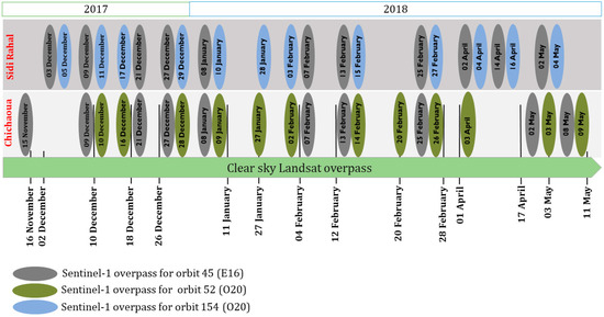
Figure 2.
Dates of the Sentinel-1 and clear sky Landsat-7/8 overpasses for both the Chichaoua and Sidi Rahal sites.
- SM data analysis
Figure 3 displays the intercomparison at Chichaoua and Sidi Rahal sites separately between the SM retrieved from remote sensing with three different approaches, and in-situ measurements: O20 for Ouaadi et al. (2020), E16 for El Hajj et al. (2016), and O19 for Ojha et al. (2019). Statistical metrics are reported in Table 1.
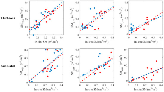
Figure 3.
Retrieved soil moisture (SM) (from left to right columns: SMO20, SME16, SMO19) versus in-situ measurements at the Chichaoua and Sidi Rahal sites. Red points correspond to dates that coincide with the same date of the Landsat overpass. Blue points correspond to dates with a one- or two-day offset with the Landsat overpass.

Table 1.
Statistical parameters for validation results of satellite retrieved soil moisture (SM) at the Chichaoua and Sidi Rahal sites.
Over the Chichaoua site, the determination coefficient (R2) was 0.72, 0.52, and 0.62. The root mean square (RMSE) was 0.04, 0.05, and 0.04 m3/m3, and the mean bias error was 0.02, 0.02, and −0.02 m3/m3 when using SMO20, SME16, and SMO19, respectively. Poorer performance was obtained over the Sidi Rahal site, where the R2 was 0.36, 0.54, and 0.45, the RMSE was 0.09, 0.11, and 0.11 m3/m3, and the MBE was −0.03, −0.08, and −0.12 m3/m3 for the O20, E16, and the O19 approaches, respectively. It can be clearly seen that the results contrasted, and the Sidi Rahal site showed a lower correlation compared to the Chichaoua site when using all three approaches.
The O20 approach seems to give good results compared to the E16 one, especially over the Chichaoua site. This may be linked to the vegetation descriptor used to describe the vegetation development within the WCM, which can affect the signal modeling, and in turn biased the derived SM. Note that the O20 approach uses interferometric coherence while E16 uses the NDVI as the vegetation descriptor within the WCM. El Hajj et al. (2016) indicated that more precise SM estimates were obtained for NDVI lower than 0.75, while the SM estimates dropped drastically for a NDVI superior to 0.75 (RMSE ~0.06 m3/m3). In addition, Ouaadi et al. (2020) analyzed the time series of predicted backscattering coefficient (σ0) by the WCM using several vegetation descriptors on wheat crop. They reported that the early saturation of NDVI at the end of the season affects the variability of the signal and showed that the dry biomass, which is highly correlated to the interferometric coherence, is the only variable that can explain the signal variation from sowing to harvest [30]. In the same vein, El Hajj et al. (2018) [59] confirmed that σ0 and SM were poorly correlated at the C-band for NDVI greater than 0.7. The poorer results obtained over the Sidi Rahal site could be explained by the stronger soil contribution linked to slightly larger incidence angles (40° and 42.2° for the O20 and E16 approaches, respectively) of the Sentinel-1 observations. In addition, it should be noted that the O20 approach has been calibrated over the Chichaoua site using ancillary field (roughness, vegetation water content, and biomass) data. Its application to another site may generate some errors, which is clearly illustrated over the Sidi Rahal site.
Results of the O19 approach (disaggregation scheme) were better than the E16 approach over the Chichaoua site, which confirms the robustness of the DisPATCh methodology over irrigated areas where the variability of SM and vegetation conditions is large [20]. However, the correlation is slightly lower over the Sidi Rahal site compared to both O20 and E16 approaches. In fact, the DisPATCh algorithm is based on the contextual methodology, which relies on determining the wet and dry temperatures within each SMAP pixel, and consequently, the soil evaporative efficiency (SEE) used for downscaling SM. Over irrigated areas, the SM variability is very large, allowing for a good determination of dry and wet conditions, and consequently, lower errors on disaggregated SM are expected. However, over rainfed areas, SM is relatively uniform over large areas as it mostly depends on large scale rainfall events, which can affect the temperature endmembers calculation and hence the SMO19 for the Sidi Rahal site, as reported by Ojha et al. (2019). In addition, the surface and atmospheric conditions can affect the performance of the present approach. One of the major issues that can explain the differences between DisPATCh and in-situ SM is the difference between SMAP and Landsat overpass times. In fact, a high repeat cycle of thermal/optical data consistent with the SMAP repeat cycle as well as with the irrigation frequency is required to improve the disaggregation process. Another major limitation that can affect the comparison is the relative coarse scale of the SMO19 pixel compared to the field size. Indeed, the Chichaoua and Sidi Rahal sites included more than one pixel of SMO19, and a simple averaging of all pixels was compared to the SM measurements. The heterogeneity within the pixel of 100 m may affect the SM estimates.
3. Model
The original TSEB is a thermal-based energy balance model described by Colaizzi et al. (2014) [60]; Elfarkh et al. (2020) [40]; Kustas and Norman, (1997) [37], and Norman et al. (1995) [36]. It solves the energy balance in the soil and vegetation separately. The plant transpiration is estimated by the Priestley Taylor (PT) formula, while the soil evaporation is calculated as a residual term of the energy balance. The PT coefficient (αPT) is one of the most sensitive parameters of TSEB as it directly controls plant transpiration and indirectly controls soil evaporation from the previously estimated transpiration. It is taken equal to 1.26 by default in optimum conditions [61]. TSEB has been modified to integrate SM as an additional constraint in the energy balance [49]. The main equations of the TSEB-SM model are presented in the Appendix A. The transpiration in TSEB-SM is based on the PT formula as in the original TSEB, while soil evaporation is presented through a soil resistance term as a function of SM. TSEB-SM adopts a calibration procedure. First, the soil parameters (arss, brss) used in the soil resistance estimates are calibrated for fc values inferior to 0.5. Then, αPT related to plant transpiration is retrieved at a daily time scale when the vegetation starts to grow (fc > 0.5). These pixel-scale calibrated (soil and vegetation) parameters are likely to improve ET estimates within the energy balance. More details are available in our previous studies [44,49].
TSEB-SM has been tested over several wheat fields in the Tensift Basin using in-situ and coarse remote sensing data (SMOS and MODIS). However, due to strong cover heterogeneity within the MODIS pixel, the use of such coarse spatial resolution data seems difficult to apply in our context, since the aim of this work was to map the energy fluxes at the field scale. Instead, high spatial resolution LST and NDVI from Landsat7/8 combined with high-resolution microwave-derived SM (retrieved by three different approaches) are incorporated simultaneously within the TSEB-SM model.
4. Results and Discussion
4.1. Classic TSEB Estimates Using Remote Sensing LST and NDVI
As TSEB-SM basically relies on the TSEB formulation, the performance of TSEB has been evaluated over the Chichaoua and Sidi Rahal sites as a benchmark for flux estimates. Figure 4 presents an intercomparison of the simulated and measured energy balance components including net radiation (Rn), ground heat flux (G), sensible (H), and latent (LE) heat fluxes. Statistical metrics are reported in Table 2. The Rn and G were well estimated by the model over the Chichaoua site. G was poorly estimated over the Sidi Rahal site, which can be explained by the empirical nature of the equation used in the model (G = cG × Rnsoil) or by errors associated with G measurements. LE was overestimated in TSEB for both sites. The RMSE was about 140 and 106 W/m2 and MBE was about 94 and 101 W/m2 for Chichaoua and Sidi Rahal, respectively. This overestimation is linked to αPT, which remains constant in TSEB for the entire agricultural season and can produce higher values of LE. The impact of αPT is more significant in the senescence phase when it is expected to drop to values below 1.26. For sensible heat flux, it can be clearly seen that the model underestimated H with a mean bias of −110 W/m2 over both sites; these results are in concordance with our previous studies [43] where they confirmed that H seems to be insensitive to any atmospheric or surface changes in the TSEB model. An additional explanation of such discrepancies in estimating H might be related to the errors associated with LST estimation. In fact, it has been shown that an error of 1 K in LST can be translated to a 50 W/m2 error in H estimates when the instantaneous energy balance model is used [62]. However, the rationale behind TSEB-SM is to correct the saturation of TSEB in the higher LE range by constraining the soil evaporation from SM observations. In practice, plant transpiration is modulated by varying the PT coefficient corresponding to the actual plant hydric status.
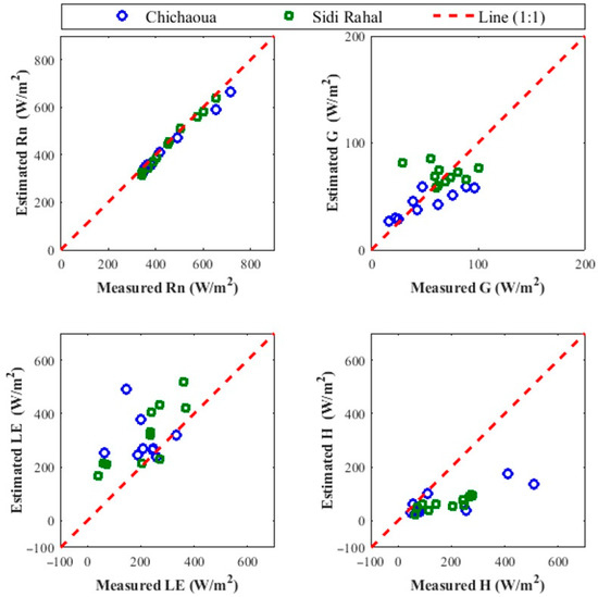
Figure 4.
Scatterplot of simulated versus observed Rn, G, LE, and H using the TSEB model at the Chichaoua and Sidi Rahal sites.
Table 2.
Statistical results (RMSE, R2, and MBE) between the modeled and measured net radiation, ground heat flux, sensible, and latent heat fluxes for Chichaoua and Sidi Rahal using the TSEB model.
4.2. TSEB-SM Estimates Using Remote Sensing SM, LST, and NDVI
In this section, the time series of retrieved αPT at the Landsat overpass time are first presented using the three SM datasets discussed previously. Then, the calibrated values are used to estimate the surface fluxes (Rn, G, H, and LE) using the TSEB-SM model. The performance of TSEB-SM in terms of the LE and H estimates was assessed against the TSEB results through a comparison with the EC measurements. Finally, we used a map of the H and LE fluxes using the TSEB-SM model over an agricultural area (named R3) mainly occupied by wheat.
Note that the original version of TSEB-SM includes a two-step calibration on the soil resistance and PT coefficient sequentially. In fact, the calibration of the parameter pair (arss,brss) requires a considerable number of SM values covering a large range (ideally from the residual SM to the SM at saturation) in a soil with fc < 0.5.
However, as above-mentioned, few SM data at the Landsat overpass were available over the entire 2017–2018 agricultural season. Over the Chichaoua site, four SMO20 values ranging between 0.24 and 0.31 m3/m3, five SME16 values ranging between 0.14 and 0.28 m3/m3, and four SMO19 ranging between 0.13 and 0.21 m3/m3 were available for fc < 0.5. The range of each SM product was small and does not represent the dry conditions, which would affect the calibration procedure. The same case occurred for the Sidi Rahal site, which involves significant uncertainties in the calibrated arss and brss. To overcome this limitation, the calibration of the pair coefficients (arss and brss) was not applied. The calibrated coefficients retrieved using in-situ data [43] were exploited for this study, which were 6.51, 3.82 for Chichaoua and 7.62, 2.43 for the Sidi Rahal site. Hence, the calibration procedure essentially relies on the retrieval of αPT at the Landsat overpass time.
4.2.1. Retrieved αPT at the Satellite Overpass Time
The transpiration in TSEB-SM is based on the PT formula as in the original TSEB. However, αPT values are retrieved at the satellite overpass time scale when the vegetation starts to grow (fc > 0.5). These calibrated values are used to estimate the surface fluxes (Rn, G, H, and LE). Figure 5 displays the retrieved αPT at the satellite overpass time superimposed with in-situ SM over Chichaoua and Sidi Rahal using the three SM retrieval approaches. Since only the days that coincide or are close to the time of the Landsat-7/8 overpasses were chosen, few data were available. Over the Chichaoua site, the retrieved αPT values varied according to the SM variabilities for the O20 and E16 approaches. The maximum of αPT was about 1.48 and 1.73 for the O20 and E16 approaches, respectively. This maximum was reached (mid-February) a few days before the peak of NDVI (end of February). The differences between the O20 and E16 approaches are related to differences in the retrieved SM values used for the inversion of αPT. For the O19 approach, the variability of αPT follows the SM variation as for both O20 and E16 approaches, but until its early peak by the end of January. This may be attributed to the uncertainties in retrieved αPT. This latter peaks again at mid-February (αPT = 1.54) and drops drastically when wheat dries out during the senescence period.
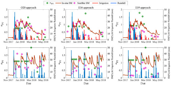
Figure 5.
Daily retrieved αPT (green points) superimposed with SM-5 cm, irrigation, and rainfall events for the three SM retrieval approaches (red points) and in-situ SM at the Chichaoua and Sidi Rahal sites.
Over the Sidi Rahal site, the frequency and amount of rainfall during 2017–2018 were important. This is well shown in the SM variability that ranged between 0.2 and 0.4 m3/m3. The αPT (calculated as an average of the inverted αPT for fc > 0.5) was almost constant until mid-February for the three SM retrieval approaches. The higher αPT value (=2) reached at the end of February (28 February) may be explained by the optimum conditions on this day. In fact, the SM retrieved from the three approaches was 0.28, 0.15, and 0.17 m3/m3 for O20, E16, and O19, respectively, LST was about 296.82 K (Tair = 294.94 K) and the root zone SM reached its saturation. These conditions promote plant transpiration up to the potential rate, and consequently higher αPT value. Overall, the results are in accordance with those found in Ait Hssaine et al. (2020) over the same field where the αPT ranged between 0.5 and 1.2 throughout the 2017–2018 season.
4.2.2. Surface Fluxes Estimates at the Field Scale
Figure 6 and Figure 7 display the scatterplot of the simulated versus measured Rn, G, H, and LE fluxes by applying the three SM retrieval approaches over the Chichaoua and Sidi Rahal sites. According to the statistical metrics reported in Table 3, a significant improvement of H and LE fluxes was noted when comparing the TSEB and TSEB-SM results. This is mainly linked to the SM constraint, which leads to a systematic and significant bias reduction on the evaporative fraction. In addition, the variability of αPT according to the actual stress conditions is able to improve the sensitivity (reduce saturation) of the energy balance model in the higher LE range. Over the Chichaoua site, Rn and G were well simulated by TSEB-SM; the mean R2 using the three SM retrieval approaches was 0.99 and 0.80; the mean RMSE was 25 and 21 W/m2; and the average MBE was −21 and −2 W/m2 for Rn and G, respectively. Additionally, it was noticed that LE was well estimated using the O20 approach with an R2 equal to 0.70, an RMSE of 38 W/m2, and MBE of −12 W/m2. In fact, Sentinel−1 and the Landsat7/8 infrequently passed over the study area on the same day. Consequently, SM with a shift of one or two days with the Landsat 7/8 overpass was chosen. These data may affect the retrieved αPT, which in turn creates the discrepancies of the LE estimates. The O19 approach produced better LE estimates compared to the O20 and E16 approaches with an R2 of about 0.85, RMSE of 21 W/m2, and low bias of −6 W/m2. This is consistent with the relatively good accuracy of SMO19 over the Chichaoua site. For the sensible heat flux H, the O20 and O19 approaches have been shown to perform well compared to the E16 approach with an R2 of about 0.94 and 0.95 and slightly lower MBE of about −9 W/m2 and −11 W/m2 for the O20 and O19 approaches, respectively.
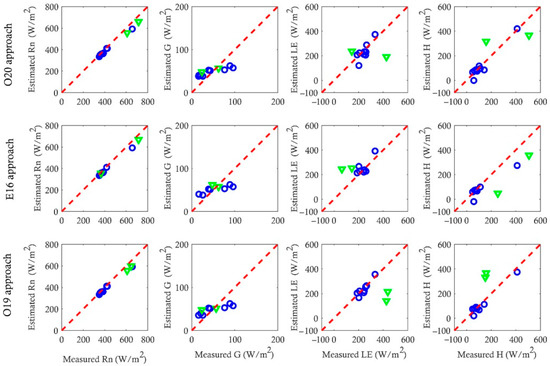
Figure 6.
Scatterplot of simulated versus observed Rn, G, LE, and H using the three SM retrieval approaches at the Chichaoua site (green points correspond to anomaly conditions).
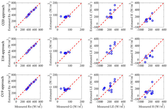
Figure 7.
Scatterplot of simulated versus observed Rn, G, LE, and H using the three approaches at the Sidi Rahal site.
Table 3.
Statistical results (RMSE, R2, and MBE) between the modeled and measured net radiation, conductive, latent, and sensible heat fluxes for Chichaoua and Sidi Rahal by applying the TSEB-SM model for the three SM retrieval approaches, separately.
Over the Chichaoua site, few points biased the correlation between the simulated and measured LE/H for the three approaches (green points). Interpreting the anomalies based on the retrieved αPT is thus needed. For the O20 approach, 1 April 2018 reports an underestimation of LE linked to a low value of αPT (=0.18) while in-situ and satellite SM was ~0.10 m3/m3 on this particular date. However, this date corresponded to a higher value of NDVI (0.69) and higher vegetation water content (VWC~4 kg/m2), meaning that αPT must be higher to predict better LE. The other anomaly was noted on 11 May 2018, which reported an overestimation of LE with an αPT value of about 0.16. This date corresponded to the senescence period when NDVI starts to decrease (NDVI = 0.23, VWC ~1 kg/m2), while the SMO20 of ~0.16 m3/m3 was higher than the in-situ SM of ~0.08 m3/m3, where this value can affect the retrieved αPT, and consequently the LE estimates. For the E16 approach, the first anomaly was revealed on 16 November 2017, when the LE was overestimated by about 181 W/m2 and the soil was almost bare (NDVI = 0.08). Nevertheless, the SME16 was about 0.13 m3/m3, which was much higher than the in-situ SM of ~0.034 m3/m3. The αPT inverted by the TSEB-SM was about 0.88, which is definitely too large for such dry conditions. LE was overestimated on 11 May 2018 by 108 W/m2 for the E16 approach. For this date, the SME16 was about 0.12 m3/m3, slightly higher than the in-situ SM of ~0.08 m3/m3. For the O19 approach, the anomalies were noted on 1 April 2018 and 17 April 2018, when LE was underestimated by about 250 W/m2. A mean difference of about 0.05 m3/m3 between the in-situ and SMO19 was noted. However, with the optimal conditions discussed previously, an αPT of 0.06 and 0.2 remains far too small to predict the correct LE estimates when vegetation is in full development and undergoes no stress.
To further investigate the possible source of errors, over the Chichaoua site, a sensitivity study of the SM impact on surface flux estimates was undertaken. Three dates were chosen: 26 December 2017, 4 February 2018, and 3 May 2018. Figure 8 illustrates the SM used as input to TSEB-SM versus the root mean square error on H and LE. Note that the values inside the rectangle represent the RMSE of H and LE using in-situ SM. For the first date, the best H and LE RMSE were obtained for SM in-situ (RMSE was about 22 and 30 W/m2 for H and LE, respectively). The errors increased for low SM, and became almost constant for high SM. This can be explained by the energy-limited conditions, meaning that high SM values do not necessarily lead to greater ET. For the second date, the lower RMSE on LE was obtained for SM = 0.15 m3/m3. On this date, the RMSE on H remained high. In contrast, the lower RMSE on H was obtained for SM = 0.35 m3/m3, while the RMSE on LE was still important for this date. For in-situ SM, sub-optimal RMSE for both H/LE was noted. For the third date, the best RMSE for both H and LE was obtained for low SM values, whereas large errors in the H and LE estimates were noted when SM exceeded 0.10 m3/m3. This sensitivity analysis confirmed the strong impact of SM data on H/LE estimates.
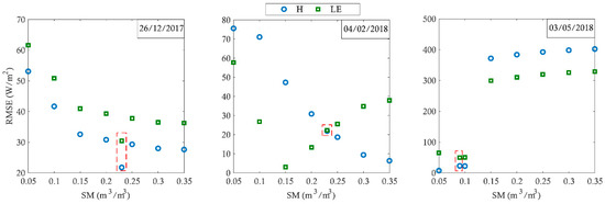
Figure 8.
SM change as input to TSEB-SM vs. the H and LE RMSE over the Chichaoua site on three selected dates.
At the Sidi Rahal site, Rn was well predicted with an average of R2, RMSE, and MBE equal to 0.99, 12 W/m2, and MBE −10 W/m2, respectively. The performance of TSEB-SM for predicting G was lower. As a simple relation based on soil net radiation is used, an error on the soil radiation estimation can be directly translated into an error in predicted G. In addition, G is widely known as a difficult component to measure, since the plates must be totally covered to avoid their exposure to sunlight. However, successive rainfall events can alter the exposure of plates, which can affect the G measurements. Unfortunately, H and LE were poorly estimated over the Sidi Rahal site for the three SM retrieval approaches, as shown in Figure 8. Indeed, the discrepancies revealed by the model for the O20 and E16 approaches were linked to the lower incidence angle (<40°), which affected the soil moisture retrieval (stronger contribution of the soil at lower incidence angles) [30] and consequently the flux estimates. The overestimation shown in the figure can mainly be linked to the higher αPT values. When using SMO19, the LE and H estimates were significantly more biased as the error associated to αPT was directly translated into H and LE uncertainties.
4.2.3. Evapotranspiration Mapping
The TSEB-SM model is constrained by the triplet LST, SM, and NDVI and uses the fc to differentiate between bare and covered soils. Its applicability over extended agricultural areas requires remote sensing data with high spatial resolution suitable to the land use classification to predict accurate ET on a field-by-field basis. To do so, microwave data with high spatial resolution and Landsat LST and NDVI were combined to map the ET over an agricultural area (named R3) mostly occupied by wheat, with some vegetables and trees are also cropped. Overall, the land classification did not affect the strategy of the TSEB-SM algorithm as the calibration of the soil/vegetation parameters was linked to the fraction cover threshold (the soil parameters were calibrated for fc < 0.5 and the PT coefficient was calibrated for fc > 0.5). An automatic weather station was installed in the R3 perimeter to provide continuous measurements of meteorological data including air temperature solar radiation, relative humidity, wind speed, and rainfall at the half-hourly time step. These data were considered unchanged and representative of the entire zone. Three different dates with contrasting conditions were chosen to have a global vision on ET throughout the season: 26 December 2017 (fc < 0.5) when the soil is almost bare (ET is mainly controlled by soil evaporation); 28 February 2018 (fc > 0.5) when the vegetation is in its full development (plant transpiration controls the ET); and 3 May 2018, which corresponds to the senescence period when wheat dries out, leading to a drastic drop of NDVI.
Microwave based-SM from the three approaches explained above were used to predict the sensible and latent heat fluxes in Figure 9, Figure 10 and Figure 11. SM from the O20 and E16 approaches were aggregated to Landsat resolution (30 m), while SM from the O19 approach was kept to a 100 m resolution and Landsat LST/NDVI was aggregated to 100 m. At the field scale, it was shown that the 100 m resolution was relatively coarse for agricultural applications in this region while using the O19 approach. To overcome this limitation, a compromise between two constraints was considered: (1) the site was carefully chosen, which is a large area dominated by wheat and the size of most fields exceeded 2 ha; and (2) the LE/H fluxes were estimated at the pixel scale and not at the field scale, so that the impact of the heterogeneity within the single pixel of 100 m will be subdued.
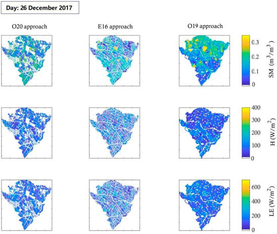
Figure 9.
SM, H, and LE maps over an irrigated perimeter located 40 km east of Marrakech named R3 using three different input SM datasets (26 December 2017).
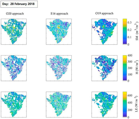
Figure 10.
Same as Figure 9, but for 28 February 2018.
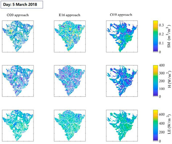
Figure 11.
Same as Figure 9, but for 3 May 2018.
One can observe that there was a remarkable variability of hydric conditions from field to field for the three dates chosen. Such a variability is related to the irrigation distribution and to sowing date differences from one field to another. Indeed, this large irrigated area is irrigated by flood, and the amount and date of irrigation is managed by the Regional Office for Agricultural Development (ORMVAH). It can take up to 15 days for the entire R3 perimeter to be irrigated, which causes the diversity in terms of hydric conditions. Note that the irrigation turns could be slightly modified if rain occurred at the date initially defined.
It should be noted that the time of the Sentinel-1 overpass does not always coincide to the Landsat-7/8 time revisit. Although, in order to apply our approach, SM with a shift of one or two days with Landsat-7/8 overpass was chosen. For the first date (26 December 2017), H ranged between 0 and 176, 6 and 164, and 12 and 165 W/m2 for the O20, E16, and O19 approaches, respectively, while LE ranged between 59 and 301, 56 and 308, and 71 and 292 W/m2 for the O20, E16, and O19 approaches, respectively. The range of values is acceptable because this date corresponds to the beginning of the season and the wheat is under development. Higher values of LE correspond to higher SM values. For the second date (28 February 2018), H varied between 0 and 310, 0 and 284, and 0 and 286 W/m2 for the O20, E16, and O19 approaches, respectively. The gap noted on the H maps was due to the negative values produced by the model. As the vegetation was in full development LE peaked in several fields and ranged between 91 and 683, 83 and 678, and 98 and 633 W/m2 for the O20, E16, and O19 approaches, respectively. Lower LE values correspond to dry conditions over bare soils that are not cropped. For the third date, H became larger because the vegetation started to dry out. The maximum of H (average of the three approaches) was around 317 W/m2, while the maximum of LE was about 535 W/m2.
5. Conclusions
The main objective of this work was to assess the gain in terms of H/LE flux estimates when integrating microwave-based SM data in a thermal-based energy balance model over an agricultural area in the Haouz Plain, central Morocco. To do so, SM products were derived from microwave remote sensing using three different approaches: the first one used the water cloud model (WCM) forced by Sentinel-1 data and the interferometric coherence to derive the above ground biomass used as a vegetation descriptor for the WCM; the second inverted the SM from Sentinel-1 radar data and the vegetation index from Sentinel-2 using a machine learning algorithm trained on a synthetic dataset simulated by the WCM; and the third approach combined the SMAP SM and Landsat optical/thermal data within a downscaling model to disaggregate SM at a 100 m resolution. The retrieved SM and Landsat LST and vegetation index were simultaneously used as input to constrain the TSEB-SM model. TSEB was chosen as the benchmark model to evaluate the TSEB-SM performance.
First, the latent (LE) and sensible (H) heat fluxes predicted by the TSEB model were evaluated by comparing them against the EC measurements. On one hand, the results showed an overestimation of LE mainly linked to the PT coefficient fixed to a constant value (=1.26). This value is valid in optimum conditions only when the vegetation undergoes no stress. On the other hand, H was underestimated by TSEB. H seems to be insensitive to any atmospheric or surface changes. To overcome this limitation, SM products in conjunction with Landsat based LST and NDVI were used to constrain the TSEB-SM model, and the PT coefficient was inverted at the daily time scale when the soil was fully covered by the vegetation. The H/LE components were well estimated compared to the original TSEB, especially over the Chichaoua site. In fact, the enhancement of the PT-based TSEB formalism by integrating SM systematically reduced the bias on the evaporative fraction. In addition, the temporal variability of αPT corrects the saturation issue of TSEB in the higher LE range. The sensitivity of LE/H to SM was also tested over the Chichaoua site for three different dates. The results showed that an error of 0.05 m3/m3 in SM generally translated into a mean error of 62 W/m2 in LE and 59 W/m2 in H. At the Sidi Rahal site, the LE and H were significantly biased, which may be explained by the soil moisture retrieval that affect the calibrated αPT. Indeed, the error associated with αPT was directly translated into H and LE.
Overall, those results are very satisfying considering the errors attributed to SM retrieval. On one hand, the 100 m resolution was larger compared to the parcel size, therefore, Sentinel-1 with a 20 m resolution was adequate to apply to our approach, whereas the offset between the Sentinel-1 and Landsat overpass generated significant errors on the H/LE estimates. However, further efforts should be made to improve the SM estimates. The next thermal missions (LSTM and TRISHNA) at high spatio-temporal resolution (three days and 50 m of resolution) will overcome this limitation. In this case, the O20 approach is suggested for SM retrieval because it is a more physical approach based on the use of Sentinel-1 data only, without the need for any ancillary data that can be restricted by weather and illumination conditions.
Finally, maps of LE and H using the three SM retrieval approaches coupled to TSEB-SM were produced over an agricultural area (named R3) mainly occupied by wheat. Three dates with contrasting conditions were selected. H seemed to be higher at the beginning of the season when the soil was almost bare or when the vegetation started to dry out, while it decreased when the vegetation was in full development. Moreover, LE reached its peak in wet conditions and in fully covered soil, while it started to decrease at the end of the season. Since it is difficult to display a network of EC stations to assess the performance of ET models, we intend, in the future, to deploy a coupled optical microwave scintillometer (XLAS MkII) to assess the performance of our approach over the entire R3 irrigation district. In addition, testing the performance of other optical indices (e.g., Enhanced vegetation index(EVI), Vegetation health Index (VHI), Vegetation Condition Index (VCI)) will be investigated in future works. Last but not least, assessing the ET dynamics at high-spatial resolution over the highly heterogeneous landscape of semi-arid agricultural areas will help to better predict the crop water needs at the field scale as well as manage the overall water resources in a sustainable manner.
Author Contributions
Conceptualization, B.A.H., A.C. and O.M.; methodology, B.A.H. and O.M.; software, B.A.H.; validation, B.A.H., O.M.; formal analysis, B.A.H. and O.M.; investigation, B.A.H. and O.M.; resources, A.C., S.E.-R., O.M.; data curation, B.A.H., N.O. (Nadia Ouaadi), N.O. (Nitu Ojha) and V.R.; writing—original draft preparation, B.A.H.; writing—review and editing, O.M., A.C., S.E.-R., J.E., S.K., N.O. (Nadia Ouaadi) and V.R.; visualization, B.A.H., A.C. and O.M.; supervision, A.C.; project administration, A.C.; funding acquisition, A.C. All authors have read and agreed to the published version of the manuscript.
Funding
This study was conducted within the framework of the Center of Remote Sensing Applications (CRSA) as well as within the joint international laboratory TREMA (https://www.lmi-trema.ma/ (accessed on 1 February 2021)) and funded by the OCP S.A. (Office Chérifien des Phosphates). The authors wish to thank the projects Rise-H2020-ACCWA (grant agreement no: 823965) and PRIMA-IDEWA and PRIMA-ALTOS for partly funding the experiments.
Institutional Review Board Statement
Not applicable.
Informed Consent Statement
Not applicable.
Data Availability Statement
The data presented in this study are available on request from the corresponding author.
Acknowledgments
The authors are deeply grateful to Omar Rafi, the owner of the “Domaine”.
Conflicts of Interest
The authors declare no conflict of interest.
Appendix A
The TSEB-SM is based on the TSEB equation in the vegetation latent heat flux () estimates:
where is the PT coefficient; the fraction of green vegetation set to 1; the psychometric constant (≈67 Pa K−1); the slope of the relationship between saturation vapor pressure and air temperature; and is the vegetation net radiation.
Unlike classic TSEB, which estimates the soil latent heat flux as a residual term of the energy balance in the soil, TSEB-SM uses the resistance formulation:
where is the saturated vapor pressure at the soil surface; is the actual air vapor pressure; is the aerodynamic resistance; is the resistance to heat flux in the boundary layer immediately above the soil surface; and is the resistance to vapor diffusion and capillary flux in the soil. is computed as a function of SM and is expressed as [63,64]:
with SM being the soil moisture in the 0–5 cm soil layer; and are two empirical parameters (to be calibrated); and is the SM at saturation expressed as [65]:
where is the sand fraction.
, , and are calibrated based on the fractional cover threshold from the SM and LST data [44].
The is first adjusted by minimizing a cost function defined by:
where and are the simulated and measured LST, respectively. The inverted is then correlated to the SM to determine the and parameters when the is lower than 0.5.
Once the soil resistance has been calibrated, the PT coefficient is retrieved at the daily time scale when is larger than 0.5 by minimizing a cost function:
An iterative loop is run on soil () and vegetation (αPT) parameters to reach the convergence of all parameters.
References
- Allen, R.G.; Tasumi, M.; Morse, A.; Trezza, R.; Wright, J.L.; Bastiaanssen, W.; Kramber, W.; Lorite, I.; Robison, C.W. Satellite-Based Energy Balance for Mapping Evapotranspiration with Internalized Calibration (METRIC)—Applications. J. Irrig. Drain. Eng. 2007, 133, 395–406. [Google Scholar] [CrossRef]
- Tasumi, M. Estimating evapotranspiration using METRIC model and Landsat data for better understandings of regional hydrology in the western Urmia Lake Basin. Agric. Water Manag. 2019, 226. [Google Scholar] [CrossRef]
- Tucker, C.J. Red and photographic infrared linear combinations for monitoring vegetation. Remote Sens. Environ. 1979, 8, 127–150. [Google Scholar] [CrossRef]
- Nouri, H.; Beecham, S.; Kazemi, F.; Hassanli, A.M. A review of ET measurement techniques for estimating the water requirements of urban landscape vegetation. Urban Water J. 2012, 10, 247–259. [Google Scholar] [CrossRef]
- Allen, R.G.; Pereira, L.S.; Howell, T.A.; Jensen, M.E. Evapotranspiration information reporting: I. Factors governing measurement accuracy. Agric. Water Manag. 2000, 78, 899–920. [Google Scholar] [CrossRef]
- Zhou, Y.; Yang, G.; Wang, S.; Wang, L.; Wang, F.; Liu, X. A new index for mapping built-up and bare land areas from Landsat-8 OLI data. Remote Sens. Lett. 2014, 5, 862–871. [Google Scholar] [CrossRef]
- Corradini, C. Soil moisture in the development of hydrological processes and its determination at different spatial scales. J. Hydrol. 2014, 516, 1–5. [Google Scholar] [CrossRef]
- Schmugge, T.J.; Kustas, W.P.; Ritchie, J.C.; Jackson, T.J.; Rango, A. Remote sensing in hydrology. Adv. Water Resour. 2002, 25, 1367–1385. [Google Scholar] [CrossRef]
- Njoku, E.G.; Jackson, T.J.; Lakshmi, V.; Member, S.; Chan, T.K.; Nghiem, S.V. Soil Moisture Retrieval From AMSR-E. IEEE Trans. Geosci. Remote Sens. 2003, 41. [Google Scholar] [CrossRef]
- Kerr, Y.H.; Waldteufel, P.; Wigneron, J.-P.; Delwart, S.; Cabot, F.; Boutin, J.; Escorihuela, M.-J.; Font, J.; Reul, N.; Gruhier, C.; et al. The SMOS Mission: New Tool for Monitoring Key Elements of the Global Water Cycle. Proc. IEEE 2010, 98. [Google Scholar] [CrossRef]
- Entekhabi, D.; Njoku, E.G.; O’Neill, P.E.; Kellogg, K.H.; Crow, W.T.; Edelstein, W.N.; Entin, J.K.; Goodman, S.D.; Jackson, T.J.; Johnson, J.; et al. The Soil Moisture Active Passive {(SMAP)} Mission. Proc. IEEE 2010, 98, 704–716. [Google Scholar] [CrossRef]
- Sabaghy, S.; Walker, J.P.; Renzullo, L.J.; Jackson, T.J. Spatially enhanced passive microwave derived soil moisture: Capabilities and opportunities. Remote Sens. Environ. 2018, 209, 551–580. [Google Scholar] [CrossRef]
- Peng, J.; Loew, A.; Merlin, O.; Verhoest, N.E.C. A review of spatial downscaling of satellite remotely sensed soil moisture. Rev. Geophys. 2017, 55. [Google Scholar] [CrossRef]
- Santi, E. An application of the SFIM technique to enhance the spatial resolution of spaceborne microwave radiometers. Int. J. Remote Sens. 2010, 31, 2419–2428. [Google Scholar] [CrossRef]
- Gevaert, A.I.; Parinussa, R.M.; Renzullo, L.J.; van Dijk, A.I.J.M.; de Jeu, R.A.M. Spatio-temporal evaluation of resolution enhancement for passive microwave soil moisture and vegetation optical depth. Int. J. Appl. Earth Obs. Geoinf. 2016, 45, 235–244. [Google Scholar] [CrossRef]
- Owe, M.; de Jeu, R.; Holmes, T. Multisensor historical climatology of satellite-derived global land surface moisture. J. Geophys. Res. Earth Surf. 2008, 113, F01002. [Google Scholar] [CrossRef]
- Chan, S.K.; Bindlish, R.; O’Neill, P.; Jackson, T.; Njoku, E.; Dunbar, S.; Chaubell, J.; Piepmeier, J.; Yueh, S.; Entekhabi, D.; et al. Development and assessment of the SMAP enhanced passive soil moisture product. Remote Sens. Environ. 2018, 204, 931–941. [Google Scholar] [CrossRef]
- Malbéteau, Y.; Merlin, O.; Molero, B.; Rüdiger, C.; Bacon, S. DisPATCh as a tool to evaluate coarse-scale remotely sensed soil moisture using localized in situ measurements: Application to SMOS and AMSR-E data in Southeastern Australia. Int. J. Appl. Earth Obs. Geoinf. 2016, 45, 221–234. [Google Scholar] [CrossRef]
- Merlin, O.; Escorihuela, M.J.; Mayoral, M.A.; Hagolle, O.; Al Bitar, A.; Kerr, Y. Self-calibrated evaporation-based disaggregation of SMOS soil moisture: An evaluation study at 3km and 100m resolution in Catalunya, Spain. Remote Sens. Environ. 2013, 130, 25–38. [Google Scholar] [CrossRef]
- Ojha, N.; Merlin, O.; Molero, B.; Suere, C.; Olivera-Guerra, L.; Ait Hssaine, B.; Amazirh, A.; Al Bitar, A.; Escorihuela, M.; Er-Raki, S. Stepwise Disaggregation of SMAP Soil Moisture at 100 m Resolution Using Landsat-7/8 Data and a Varying Intermediate Resolution. Remote Sens. 2019, 11, 1863. [Google Scholar] [CrossRef]
- Das, K.C.; Singh, J.; Hazra, J.; Sheraton, L.C. Development of a High Resolution Soil Moisture for Precision Agriculture in India. In Proceedings of the 14th International Conference on Precision Agriculture, Monteral, QC, Canada, 26–27 June 2018; pp. 1–10. [Google Scholar]
- Ali Eweys, O.; José Escorihuela, M.; Villar, J.M.; Er-Raki, S.; Amazirh, A.; Olivera, L.; Jarlan, L.; Khabba, S.; Merlin, O. Disaggregation of SMOS Soil Moisture to 100 m Resolution Using MODIS Optical/Thermal and Sentinel-1 Radar Data: Evaluation over a Bare Soil Site in Morocco. Remote Sens. 2017, 9, 1155. [Google Scholar] [CrossRef]
- Das, N.N.; Entekhabi, D.; Njoku, E.G. An algorithm for merging SMAP radiometer and radar data for high-resolution soil-moisture retrieval. IEEE Trans. Geosci. Remote Sens. 2011, 49, 1504–1512. [Google Scholar] [CrossRef]
- Chakrabarti, S.; Judge, J.; Bongiovanni, T.; Rangarajan, A.; Ranka, S. Disaggregation of Remotely Sensed Soil Moisture in Heterogeneous Landscapes Using Holistic Structure-Based Models. IEEE Trans. Geosci. Remote Sens. 2016, 54, 4629–4641. [Google Scholar] [CrossRef]
- Sabaghy, S.; Walker, J.P.; Renzullo, L.J.; Akbar, R.; Chan, S.; Chaubell, J.; Das, N.; Dunbar, R.S.; Entekhabi, D.; Gevaert, A.; et al. Comprehensive analysis of alternative downscaled soil moisture products. Remote Sens. Environ. 2020, 239. [Google Scholar] [CrossRef]
- Torres, R.; Snoeij, P.; Geudtner, D.; Bibby, D.; Davidson, M.; Attema, E.; Potin, P.; Rommen, B.Ö.; Floury, N.; Brown, M.; et al. GMES Sentinel-1 mission. Remote Sens. Environ. 2012, 120, 9–24. [Google Scholar] [CrossRef]
- Ferrazzoli, P.; Paloscia, S.; Pampaloni, P.; Schiavon, G.; Solimini, D.; Coppo, P. Sensitivity of Microwave Measurements to Vegetation Biomass and Soil Moisture Content: A Case Study. IEEE Trans. Geosci. Remote Sens. 1992, 30, 750–756. [Google Scholar] [CrossRef]
- Ulaby, F.T.; Batlivala, P.P.; Dobson, M.C. Microwave Backscatter Dependence on Surface Roughness, Soil Moisture, and Soil Texture: Part I–Bare Soil. IEEE Trans. Geosci. Electron. 1978, 16, 286–295. [Google Scholar] [CrossRef]
- Bousbih, S.; Zribi, M.; Lili-Chabaane, Z.; Baghdadi, N.; El Hajj, M.; Gao, Q.; Mougenot, B. Potential of sentinel-1 radar data for the assessment of soil and cereal cover parameters. Sensors 2017, 17, 2617. [Google Scholar] [CrossRef]
- Ouaadi, N.; Jarlan, L.; Ezzahar, J.; Zribi, M.; Khabba, S.; Bouras, E.; Bousbih, S.; Frison, P.L. Monitoring of wheat crops using the backscattering coefficient and the interferometric coherence derived from Sentinel-1 in semi-arid areas. Remote Sens. Environ. 2020, 251, 112050. [Google Scholar] [CrossRef]
- Attema, E.P.W.; Ulaby, F.T. Vegetation modeled as a water cloud. Radio Sci. 1978, 13, 357–364. [Google Scholar] [CrossRef]
- Kumar, S.V.; Peters-Lidard, C.D.; Santanello, J.A.; Reichle, R.H.; Draper, C.S.; Koster, R.D.; Nearing, G.; Jasinski, M.F. Evaluating the utility of satellite soil moisture retrievals over irrigated areas and the ability of land data assimilation methods to correct for unmodeled processes. Hydrol. Earth Syst. Sci. 2015, 19, 4463–4478. [Google Scholar] [CrossRef]
- Bai, X.; He, B.; Li, X.; Zeng, J.; Wang, X.; Wang, Z.; Zeng, Y.; Su, Z. First assessment of Sentinel-1A data for surface soil moisture estimations using a coupled water cloud model and advanced integral equation model over the Tibetan Plateau. Remote Sens. 2017, 9, 714. [Google Scholar] [CrossRef]
- El Hajj, M.; Baghdadi, N.; Zribi, M.; Belaud, G.; Cheviron, B.; Courault, D.; Charron, F. Soil moisture retrieval over irrigated grassland using X-band SAR data. Remote Sens. Environ. 2016, 176, 202–218. [Google Scholar] [CrossRef]
- Baghdadi, N.; El Hajj, M.; Zribi, M.; Bousbih, S. Calibration of the Water Cloud Model at C-Band for Winter Crop Fields and Grasslands. Remote Sens. 2017, 9, 969. [Google Scholar] [CrossRef]
- Norman, J.M.; Kustas, W.P.; Humes, K.S. Source approach for estimating soil and vegetation energy fluxes in observations of directional radiometric surface temperature. Agric. For. Meteorol. 1995, 77, 263–293. [Google Scholar] [CrossRef]
- Kustas, W.P.; Norman, J.M. A two-source approach for estimating turbulent fluxes using multiple angle thermal infrared observations. Water Resour. Res. 1997, 33, 1495–1508. [Google Scholar] [CrossRef]
- Kustas, W.P.; Norman, J.M. Evaluation of soil and vegetation heat flux predictions using a simple two-source model with radiometric temperatures for partial canopy cover. Agric. For. Meteorol. 1999, 94, 13–29. [Google Scholar] [CrossRef]
- Colaizzi, P.D.; Kustas, W.P.; Anderson, M.C.; Agam, N.; Tolk, J.A.; Evett, S.R.; Howell, T.A.; Gowda, P.H.; O’Shaughnessy, S.A. Two-source energy balance model estimates of evapotranspiration using component and composite surface temperatures q. Adv. Water Resour. 2012, 50, 134–151. [Google Scholar] [CrossRef]
- Elfarkh, J.; Ezzahar, J.; Er-Raki, S.; Simonneaux, V.; Ait Hssaine, B.; Rachidi, S.; Brut, A.; Rivalland, V.; Khabba, S.; Chehbouni, A.; et al. Multi-Scale Evaluation of the TSEB Model over a Complex Agricultural Landscape in Morocco. Remote Sens. 2020, 12, 1181. [Google Scholar] [CrossRef]
- Gan, G.; Gao, Y. Estimating time series of land surface energy fluxes using optimized two source energy balance schemes: Model formulation, calibration, and validation. Agric. For. Meteorol. 2015, 208, 62–75. [Google Scholar] [CrossRef]
- Yao, Y.; Liang, S.; Yu, J.; Zhao, S.; Lin, Y.; Jia, K.; Zhang, X.; Cheng, J.; Xie, X.; Sun, L.; et al. Differences in estimating terrestrial water flux from three satellite-based Priestley-Taylor algorithms. Int. J. Appl. Earth Obs. Geoinf. 2017, 56, 1–12. [Google Scholar] [CrossRef]
- Ait Hssaine, B.; Merlin, O.; Rafi, Z.; Ezzahar, J.; Jarlan, L.; Khabba, S.; Er-Raki, S. Calibrating an evapotranspiration model using radiometric surface temperature, vegetation cover fraction and near-surface soil moisture data. Agric. For. Meteorol. 2018, 256–257, 104–115. [Google Scholar] [CrossRef]
- Ait Hssaine, B.; Merlin, O.; Ezzahar, J.; Ojha, N.; Er-Raki, S.; Khabba, S. An evapotranspiration model self-calibrated from remotely sensed surface soil moisture, land surface temperature and vegetation cover fraction: Application to disaggregated SMOS and MODIS data. Hydrol. Earth Syst. Sci. 2020, 24, 1781–1803. [Google Scholar] [CrossRef]
- Jarlan, L.; Khabba, S.; Er-Raki, S.; Le Page, M.; Hanich, L.; Fakir, Y.; Merlin, O.; Mangiarotti, S.; Gascoin, S.; Ezzahar, J.; et al. Remote Sensing of Water Resources in Semi-Arid Mediterranean Areas: The joint international laboratory TREMA. Int. J. Remote Sens. 2015, 36, 4879–4917. [Google Scholar] [CrossRef]
- Chehbouni, A.; Escadafal, R.; Duchemin, B.; Boulet, G.; Simonneaux, V.; Dedieu, G.; Mougenot, B.; Khabba, S.; Kharrou, H.; Maisongrande, P.; et al. An integrated modelling and remote sensing approach for hydrological study in arid and semi-arid regions: The SUDMED Programme. Int. J. Remote Sens. 2008, 29, 5161–5181. [Google Scholar] [CrossRef]
- Er-Raki, S.; Chehbouni, A.; Guemouria, N.; Duchemin, B.; Ezzahar, J.; Hadria, R. Combining FAO-56 model and ground-based remote sensing to estimate water consumptions of wheat crops in a semi-arid region. Agric. Water Manag. 2007, 87, 41–54. [Google Scholar] [CrossRef]
- Amazirh, A.; Merlin, O.; Er-Raki, S.; Gao, Q.; Rivalland, V.; Malbeteau, Y.; Khabba, S.; Escorihuela, M.J. Retrieving surface soil moisture at high spatio-temporal resolution from a synergy between Sentinel-1 radar and Landsat thermal data: A study case over bare soil. Remote Sens. Environ. 2018, 211, 321–337. [Google Scholar] [CrossRef]
- Ait Hssaine, B.; Ezzahar, J.; Jarlan, L.; Merlin, O.; Khabba, S.; Brut, A.; Er-Raki, S.; Elfarkh, J.; Cappelaere, B.; Chehbouni, G. Combining a Two Source Energy Balance Model Driven by MODIS and MSG-SEVIRI Products with an Aggregation Approach to Estimate Turbulent Fluxes over Sparse and Heterogeneous Vegetation in Sahel Region (Niger). Remote Sens. 2018, 10, 974. [Google Scholar] [CrossRef]
- Rafi, Z.; Merlin, O.; Le Dantec, V.; Khabba, S.; Mordelet, P.; Er-Raki, S.; Amazirh, A.; Olivera-Guerra, L.; Ait Hssaine, B.; Simonneaux, V.; et al. Partitioning evapotranspiration of a drip-irrigated wheat crop: Inter-comparing eddy covariance-, sap flow-, lysimeter- and FAO-based methods. Agric. For. Meteorol. 2019, 265, 310–326. [Google Scholar] [CrossRef]
- Burba, G. Eddy Covariance Method for Scientific, Industrial, Agricultural, and Regulatory Applications: A Field Book on Measuring Ecosystem Gas Exchange and Areal Emission Rates; LI-Cor Biosciences: Lincoln, NE, USA, 2013. [Google Scholar]
- Tardy, B.; Rivalland, V.; Huc, M.; Hagolle, O.; Marcq, S.; Boulet, G. A Software Tool for Atmospheric Correction and Surface Temperature Estimation of Landsat Infrared Thermal Data. Remote Sens. 2016, 8, 696. [Google Scholar] [CrossRef]
- Berk, A.; Anderson, G.P.; Acharya, P.K.; Bernstein, L.S.; Muratov, L.; Lee, J.; Fox, M.J.; Adler-Golden, S.M.; Chetwynd, J.H.; Hoke, M.L.; et al. MODTRAN5: A Reformulated Atmospheric Band Model with Auxiliary Species and Practical Multiple Scattering Options. In Proceedings of the Multispectral and Hyperspectral Remote Sensing Instruments and Applications II, Honolulu, HI, USA, 20 January 2005; Volume 5655, p. 13. [Google Scholar]
- Dee, D.P.; Uppala, S.M.; Simmons, A.J.; Berrisford, P.; Poli, P.; Kobayashi, S.; Andrae, U.; Balmaseda, M.A.; Balsamo, G.; Bauer, P.; et al. The ERA-Interim reanalysis: Configuration and performance of the data assimilation system. Q. J. R. Meteorol. Soc. 2011, 137, 553–597. [Google Scholar] [CrossRef]
- Sobrino, J.A.; Jiménez-Muñoz, J.C.; Paolini, L. Land surface temperature retrieval from LANDSAT TM 5. Remote Sens. Environ. 2004, 90, 434–440. [Google Scholar] [CrossRef]
- Wittich, K.P. Some simple relationships between land-surface emissivity, greenness and the plant cover fraction for use in satellite remote sensing. Int. J. Biometeorol. 1997, 41, 58–64. [Google Scholar] [CrossRef]
- Jarlan, L.; Mougin, E.; Frison, P.L.; Mazzega, P.; Hiernaux, P. Analysis of ERS wind scatterometer time series over Sahel (Mali). Remote Sens. Environ. 2002, 81, 404–415. [Google Scholar] [CrossRef]
- Molero, B.; Merlin, O.; Malbéteau, Y.; Al Bitar, A.; Cabot, F.; Stefan, V.; Kerr, Y.; Bacon, S.; Cosh, M.H.; Bindlish, R.; et al. SMOS disaggregated soil moisture product at 1 km resolution: Processor overview and first validation results. Remote Sens. Environ. 2016, 180, 361–376. [Google Scholar] [CrossRef]
- El Hajj, M.; Baghdadi, N.; Bazzi, H.; Zribi, M. Penetration Analysis of SAR Signals in the C and L Bands for Wheat, Maize, and Grasslands. Remote Sens. 2018, 11, 31. [Google Scholar] [CrossRef]
- Colaizzi, P.D.; Tolk, J.A.; Evett, S.R.; Howell, T.A. Two-Source Energy Balance Model to Calculate E, T, and ET: Comparison of Priestley-Taylor and Penman-Monteith Formulations and Two Time Scaling Methods. Trans. ASABE 2014, 57, 479–498. [Google Scholar] [CrossRef]
- Priestley, C.H.B.; Taylor, R.J. On the Assessment of Surface Heat Flux and Evaporation Using Large-Scale Parameters. Mon. Weather Rev. 1972, 100, 81–92. [Google Scholar] [CrossRef]
- Chehbouni, A.; Watts, C.; Kerr, Y.H.; Dedieu, G.; Rodriguez, J.-C.; Santiago, F.; Cayrol, P.; Boulet, G.; Goodrich, D.C. lMethods to aggregate turbulent fluxes over heterogeneous surfaces: Application to SALSA data set in Mexico. Agric. For. Meteorol. 2000, 105, 133–144. [Google Scholar] [CrossRef]
- Sellers, P.J.; Heiser, M.D.; Hall, F.G. Relations between surface conductance and spectral vegetation indexes at intermediate (100 m2 to 15 km2) length scales. J. Geophys. Res. 1992, 97, 19033–19059. [Google Scholar] [CrossRef]
- Chirouze, J.; Boulet, G.; Jarlan, L.; Fieuzal, R.; Rodriguez, J.C.; Ezzahar, J.; Bigeard, G.; Merlin, O. Intercomparison of four remote-sensing-based energy balance methods to retrieve surface evapotranspiration and water stress of irrigated fields in semi-arid climate. Hydrol. Earth Syst. Sci. 2014, 18, 1165–1188. [Google Scholar] [CrossRef]
- Cosby, B.J.; Hornberger, G.M.; Clapp, R.B.; Ginn, T.R. A Statistical Exploration of the Relationships of Soil Moisture Characteristics to the Physical Properties of Soils. Water Resour. Res. 1984, 20, 682–690. [Google Scholar] [CrossRef]


Publisher’s Note: MDPI stays neutral with regard to jurisdictional claims in published maps and institutional affiliations. |
© 2021 by the authors. Licensee MDPI, Basel, Switzerland. This article is an open access article distributed under the terms and conditions of the Creative Commons Attribution (CC BY) license (http://creativecommons.org/licenses/by/4.0/).