Estimating Canopy Density Parameters Time-Series for Winter Wheat Using UAS Mounted LiDAR

Abstract

Monitoring of canopy density with related metrics such as leaf area index (LAI) makes a significant contribution to understanding and predicting processes in the soil–plant–atmosphere system and to indicating crop health and potential yield for farm management. Remote sensing methods using optical sensors that rely on spectral reflectance to calculate LAI have become more mainstream due to easy entry and availability. Methods with vegetation indices (VI) based on multispectral reflectance data essentially measure the green area index (GAI) or response to chlorophyll content of the canopy surface and not the entire aboveground biomass that may be present from non-green elements that are key to fully assessing the carbon budget. Methods with light detection and ranging (LiDAR) have started to emerge using gap fraction (GF) to estimate the plant area index (PAI) based on canopy density. These LiDAR methods have the main advantage of being sensitive to both green and non-green plant elements. They have primarily been applied to forest cover with manned airborne LiDAR systems (ALS) and have yet to be used extensively with crops such as winter wheat using LiDAR on unmanned aircraft systems (UAS). This study contributes to a better understanding of the potential of LiDAR as a tool to estimate canopy structure in precision farming. The LiDAR method proved to have a high to moderate correlation in spatial variation to the multispectral method. The LiDAR-derived PAI values closely resemble the SunScan Ceptometer GAI ground measurements taken early in the growing season before major stages of senescence. Later in the growing season, when the canopy density was at its highest, a possible overestimation may have occurred. This was most likely due to the chosen flight parameters not providing the best depictions of canopy density with consideration of the LiDAR’s perspective, as the ground-based destructive measurements provided lower values of PAI. Additionally, a distinction between total LiDAR-derived PAI, multispectral-derived GAI, and brown area index (BAI) is made to show how the active and passive optical sensor methods used in this study can complement each other throughout the growing season.

1. Introduction

Leaf area index (LAI) is a popular metric used to monitor crop biomass over the growing season. It is a key biophysical parameter for modeling mass and energy exchange between the biosphere and atmosphere [1]. LAI is intrinsically connected to biophysical processes such as photosynthesis, evaporation and transpiration, rainfall interception, and carbon flux [2]. LAI is widely used in crop simulation to assist in crop yield modeling and irrigation management [3]. Improving upon LAI measurement is important, especially for agricultural systems, as they are under strong pressure due to the changing climate.

LAI is the ratio of the total one-sided leaf area per unit of horizontal ground surface area (dimensionless). It can be distinguished into two subcategories. These are green leaf area index (GLAI), consisting of the green photosynthetically active leaves, and brown leaf area index (BLAI), which is those areas of brown, senescent leaves losing photosynthetic function [1,4]. There are further, closely related terms that broaden the elements of consideration beyond the plant leaf. Green area index (GAI) accounts for all green elements, including not only leaves but also other photosynthetic organs that contain chloroplasts, such as stems and reproductive organs [3]. It can be assumed that brown area index (BAI) refers to those areas consisting of any non-green elements within the plant canopy. Plant area index (PAI) is in reference to all plant elements, including green and non-green portions [3]. The definitions of these LAI-related terms are important to this study as different ones are mentioned based on the sensor and method used.

The majority of remote sensing methods use passive optical sensors with ratios of different spectral reflectances to calculate LAI [1,3,5]. Classically, the calculations are based on vegetation indices such as the normalized difference vegetation index (NDVI), which is sensitive to chlorophyll absorption [6]. This often becomes a measurement of GAI which relies on the plant pigment [5]. These techniques may be impacted by the illumination conditions during collection [7] along with background elements [6,8]. Cereal crops, such as winter wheat, begin browning with their spectral reflectance becoming similar to that of soil as they approach senescence, where the greenness no longer reflects the whole surface area of the aboveground biomass, i.e., PAI, and passive optical methods are challenged [5]. This can occur early in the growing season for crops during warm dry summer periods, which is a common case for rainfed agroecosystems in temperate or Mediterranean climates [5]. Some studies have indicated that hyperspectral data are no better than broadband multispectral data in LAI estimations and that senescent brown vegetation is usually ignored because optical methods are not calibrated for it [3,5,9]. Senescent leaves can constitute a large portion of the aboveground biomass and are important in understanding the carbon cycle [10]. It is also helpful for the farmers to know when, where, and how much of their crop is affected by stress due to drought, pests, or other damages before harvesting [5]. However, it is suggested that GAI is the most crucial for crop yield prediction [3]. With this in mind, being able to estimate both GAI and BAI could provide a more complete picture for crop management.

Ground-based methods for the estimation of LAI include digital hemispherical photography (DHP) from cameras with fisheye lenses [3,11,12], ceptometry [13,14], or devices such as the LAI-2000/2200 plant canopy analyzer (LI-COR Biosciences, Lincoln, NE, USA) [3,15,16,17]. These non-destructive methods rely on the gap fraction (GF) theory and radiation transmission. GF is defined as the fraction of light passing through the canopy without encountering foliage or other plant elements [2]. Inaccuracies are known to occur from circumstances such as scattered radiation [18] and the lack of calibration for leaf clumping [19]. These factors are not always considered or corrected. However, even when clumping corrections are used, it comes from prior knowledge of the clumping parameter, which is not universally applicable [19]. When using the LAI-2000, underestimations of 17% to over 40%, likely due to woody elements, have been experienced in a past study [16] and have had underestimations of 18% in another study after correction for wood area [17]. Errors between 10% and 20% for forests and 10% and 15% for crops have been experienced when using LAI 2200 and DHP [3,20,21,22,23,24]. Ceptometry methods, based on the measurement of average photosynthetically active radiation under a plant canopy using many individual light sensors, have shown underestimations in maize with a low–medium range of LAI [13]. However, others have demonstrated LAI estimates of sugarcane within 90% of what can be obtained with destructive measurements [25]. Ground-based methods are time-consuming, with little community consensus on measurement methods, sampling scales, and frequencies [3]. For regional-scale monitoring, aerial and space-borne remote sensing is preferred as it provides a more complete picture of a study area’s LAI values and variation.

In contrast to typical passive multispectral methods, light detection and ranging (LiDAR) can retrieve signals from the canopy, the whole plant, and the ground. LiDAR’s ability to penetrate through vegetation canopy tops is often used for height measurements, to map underlying terrain, or even to measure tree trunk diameters [26,27,28]. It is also possible to relate the rate at which these signals pass through gaps in the canopy, essentially applying GF principles to LiDAR, that is reflective of vegetation density that can be related to LAI. Studies have found that LiDAR-derived LAI has performed well by comparison with ground collection methods such as LAI-2200 [3]. It is suggested to be a better indicator of the three-dimensional plant structure as opposed to passive optical methods that mainly obtain top surface information with two-dimensional data [2]. LiDAR has the potential to estimate the complete aboveground biomass of the plant, regardless of its pigment or photosynthetic state.

Several studies have shown how manned airborne LiDAR scanning (ALS) can be used to estimate LAI in forestry [29,30,31,32,33,34]. Various attributes of LiDAR have been exploited to examine the canopy structure and density. Distinctions between echoes, signal intensity, and ground points have all been used within methods to derive LAI. These methods have proven to provide indications of suitably accurate LAI estimations. In one study [34], ALS data were used to estimate LAI and gap fraction for a forest and compared against estimations made from hyperspectral data, and R² > 0.77 was found. In [32], a performance with a R² of 0.67 was exhibited using Beer–Lambert equations. However, LiDAR-derived LAI is subject to inaccuracies depending on the vegetation cover and optimization of the surrounding methods. There is a lack of investigations into optimizing collection and processing parameters for LiDAR retrieval of LAI [32]. Overestimations are known to occur when the vegetation density is too high for the LiDAR signal to reach the ground. In the study of [30], overestimations of 3.1–4.6% were experienced, which increased considerably with scan angles over 32 degrees. The higher the scan angle, the further the signal must travel through the canopy before reaching the ground. Flight parameterization is important in ensuring a complete picture of the canopy density with the most inclusive perspectives that will result in the best ratio of gap probability to mitigate overestimation [32]. This can be related to flight line directions and spacing, altitude, scan angles, and the particular LiDAR sensor used during data acquisition [32]. There is a lack of understanding and distinction between which parameters to use in collection and processing based on the sensor used and vegetation being monitored [3,32]. There is a strong need for further research that includes more vegetation types and the investigation and improvement of various flight parameters and LiDAR features. Additionally, the methods are mainly manned ALS, which can have large LiDAR signal footprints pertaining to the higher flight altitudes and principles of beam divergence and can fail to capture the full gap-size distribution due to not being able to take advantage of small gaps in the canopy [1]. Unmanned aircraft systems (UAS) present the possibility of flights with lower altitudes, lower costs, higher flexibility, and smaller footprint sizes.

In the past few years, LiDAR technology has seen a major development in ultra-light laser scanning systems, enabling them to be more commonly mounted on UAS platforms [10]. Predominantly, UAS is used in combination with passive optical sensors because this is more affordable, and with the increase in the quality and availability of surface from motion (SfM) software, these sensors are able to create point clouds similar to those produced with LiDAR [35]. However, unlike LiDAR, they are unable to sense shadowed areas or through gaps and even suffer from over-smoothing of the data [35,36,37]. LiDAR systems for UAS are becoming increasingly more affordable with new user-friendly software, making them a more competitive solution [38]. Ultimately, UAS provide more flexibility, with compact sizes and accessibility that can provide increased temporal resolution. Being independent of cloud cover, UAS is sometimes the only means of obtaining the appropriate temporal resolution desired for a growing season [39].

Deery et al. (2021) [40] have shown the effectiveness of estimating crop metrics such as LAI throughout time using LiDAR via a ground buggy. Additionally, UAS-mounted LiDAR has been used to estimate crop density with a ratio of canopy signal returns to all signal returns to improve their biomass model [41]. To the best of our knowledge, there are no studies using a UAS-mounted LiDAR system to estimate crop PAI in relation to canopy density in a time-series throughout the growing season. This study uses the proven method of GF for PAI, previously used with ALS in forestry [32], and tests its potential with UAS and winter wheat throughout the growing season. Since the crop in this study is winter wheat with the probability of reaching senescence heterogeneously early in the growing season, the nature of multispectral data to calculate GAI is used to show the differences and similarities in methods and to provide a new method when needing to distinguish between PAI, GAI, and BAI. This shows that a combination of passive optical and LiDAR can yield improved characterization of canopy structure, as demonstrated in previous studies [42,43,44,45].

2. Materials and Methods

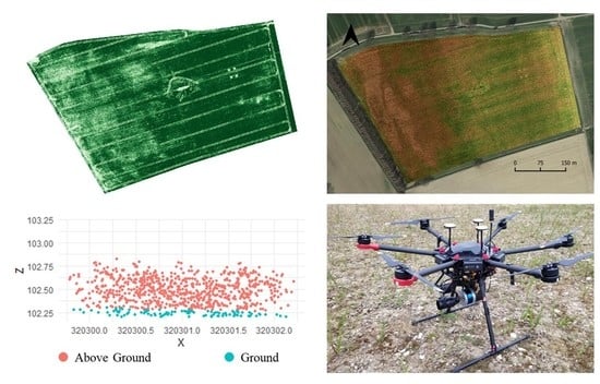
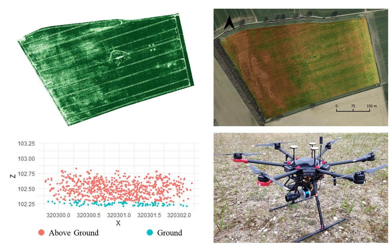
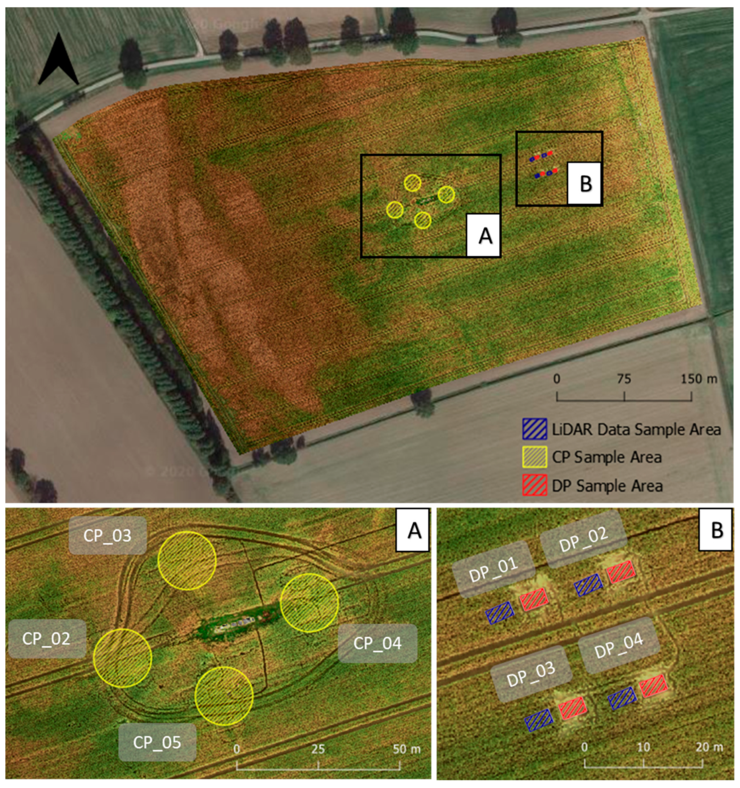
2.1. Study Area

The study was conducted at the Integrated Carbon Observation System (ICOS) Class 1 ecosystem site DE-RuS (https://www.icos-cp.eu) in Selhausen, Germany (50°51′56″N 6°27′ 03″E) with a winter wheat (Triticum aestivum) field of approximately ten hectares. It is part of the Terrestrial Environmental Observatories (TERENO) network [46] and has been selected as a Supersite by the Committee on Earth Observation Satellites (CEOS) Land Product Validation subgroup. The growing period of the winter wheat, from emergence to harvest, was approximately from October to the end of July. The field ranges from 101 m in the west to 103 m above mean sea level (MSL) in the east, with an average annual precipitation of 715 mm and average temperature of 10.2 °C. The soil is composed of Pleistocene loess and translocated loess from the Holocene, along with sand and gravels at the lower depths, which were discovered at this site through previous geophysical studies [47]. The west side of the field has increased sand and gravel amounts that are at shallower depths, which has been shown to cause heterogeneity among the crops during periods of water scarcity [47]. Likewise, the same field was previously observed using a terrestrial laser scanner (TLS) in a study for crop height estimations [48]. This study’s resulting maps show crop height patterns that appear to be in agreement with the soil properties and can be used to form prior knowledge and assumptions about the patterns in crop structure at this particular field.

2.2. Data Acquisition

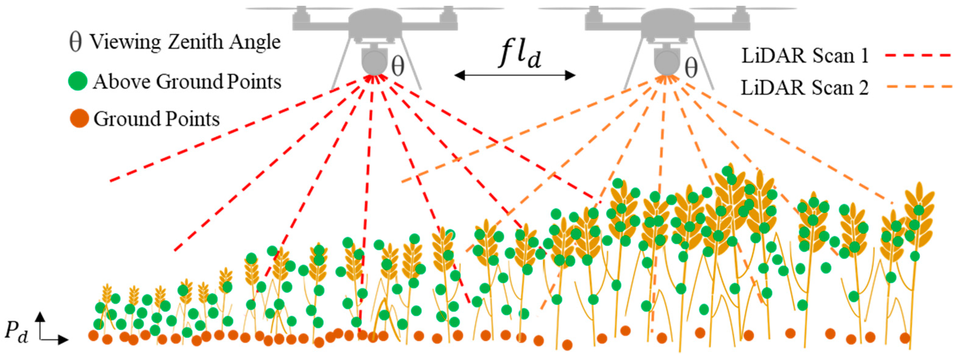
2.2.1. UAS and Sensors

Two sensors were used in this study, a YellowScan Surveyor LiDAR and a Micasense RedEdge-M multispectral sensor, each mounted on a DJI Matrice 600, as seen in Figure 1. The LiDAR unit is composed of a Velodyne LiDAR puck, onboard computer, Inertial Measuring Units (IMU), and Global Navigation Satellite System (GNSS) receiver. The GNSS-Inertial solution is from Applanix APX-15. Ranging data were provided by the LiDAR puck/scanner. The variations in attitude were measured by the IMU, and positioning was provided by the GNSS, which also provided time synchronization for all the sensors. This multi-sensor system provides precision capable of direct georeferencing [38]. Point density of the scanned surface depends on the flight altitude, speed, and flight line spacing of the aircraft. The RedEdge-M is a five narrowband multispectral camera. The spectrum is mapped in blue (465–485 nm), green (550–570 nm), red (663–673 nm), red-edge (712–722 nm), and near infrared (NIR) (820–86 nm) bands. Each has a focus length of 5.4 mm, with a 46-degree field of view (FOV). Aside from the sensors, the setup consists of a GNSS and Downwelling Light Sensor (DLS) for georeferencing and sun/cloud corrections.

The DJI Matrice 600 is a hexacopter of 17 × 15 × 7 cm in dimensions and a weight of 10 kilograms (kg). The payload capacity is 5.5–6 kg, making it possible to easily carry the 1.6-kg LiDAR system in addition to an RGB camera, which could be replaced with another sensor such as the 0.17-kg Micasense Rededge-M in future use.

2.2.2. Data Acquisition and Initial Processing

Data acquisition took place from April 1 through July 21 of 2020 and consisted of eight flight campaigns, once every two weeks. All LiDAR flights were performed at 50-m height above ground level (AGL) and at a ground speed of 5 m/s, which was balanced between coverage, overlaps, and scan angles. The approximate point density with these parameters is 85 pts/sqm, with an accuracy of 5 cm, as specified in the YelllowScan user manual. The flight speed on the second campaign (14.04.2020) was 7 m/s and had to be disregarded due to lack of resulting point density. Flight parameters varied earlier in the growing season as canopy density estimations were not the focus and they depended on the project scope at the time. Scan angles of 35 degrees on both sides, for a FOV of 70 degrees, were used to be similar to parameters used in a past ALS study for LAI [33] and proved to result in favorable values when compared to GAI earlier in the growing season before senescence. This FOV gave an approximate overlap of 60%. The first flight campaigns (01.04.2020–12.05.2020) were performed at larger flight line distances and a 60-degree scan angle had to be used to achieve similar overlaps and point density. There was a low amount of signal returns from the vegetation when lower scan angles were used for these earlier campaigns.

The LiDAR data were processed using YellowScan’s CloudStation software to process the point cloud data (LASer files) for each flight strip for alignment and georeferencing by applying corrections through GNSS offset (lever-arms), sensor angle (boresight), and GNSS post-processing with precise position techniques [10]. The post-processing solution for direct georeferencing was established using a smoothed best estimated trajectory (SBET) file from Applanix’s PosPac software with the use of a Virtual Reference Station (VRS) triangulated from Trimble’s network of reference stations.

The multispectral data were collected on the same day and directly after the LiDAR flights. However, these flights were conducted at an altitude of 100 m AGL and at a flight speed of 6 m/s. Parameters for an image forward and side overlap of approximately 90% were used. Before and after each flight, spectral calibration was performed with a reflectance panel. Ground control points were used for georeferencing. The Micasense multispectral imagery was stitched into orthomosaics for each band of the camera using photogrammetry and computer vision methods in Pix4D (Pix4D, Lausanne, Switzerland). The orthomosaics were further manually aligned and resampled to 16 cm in post-processing to be consistent with the lowest-resolution multispectral data as the first two flights in the growing season were flown at higher altitudes.

2.2.3. Ground Sampling

For comparison to the LiDAR-derived PAI, ground measurements from the ICOS site were used. All aboveground biomass measurements at the site were carried out in accordance with the ICOS protocol [49]. Measurements based on two different methods and several plot locations were performed. Repeated non-destructive GAI measurements were carried out with a linear ceptometer (SS1 SunScan Canopy Analysis System, Delta-T Devices Ltd, Campbridge, UK) throughout the growing season (08.04.2020, 06.05.2020, 28.05.2020, 22.06.2020, 02.07.2020) at four plot locations in the center of the field, deemed the Continuous Measurement Plots (CPs, see Figure 2). On each of the measurement days mentioned above, a total of 36 ceptometer measurements distributed over three sublocations were carried out for each plot and subsequently averaged to a single GAI value representative of the respective plot (CP 02-05). Destructive measurements were conducted on a single day near the end of the growing season (07.07.2020) at four locations, deemed the Destructive Measurement Plots (DPs, see Figure 2), in the eastern part of the field. Here, all biomass in each of the four plots with a size of 5.4 m², respectively, was harvested and analyzed in the lab. Metrics on green and non-green leaf, stem, and ear samples were derived using an area meter (LI-3100, LI-COR Biosciences, Lincoln, NE, USA) for subsamples of 10% of the fresh weight of the full sample from the respective plot. The flat surfaces, such as leaves, were determined directly by the LI-3100 area meter and the non-flat was determined by calculating the hemi-surface area with basic dimensions of the structure to approximate its geometric volume. The combination of these measurements was used to represent PAI and GAI. These ground measurements are used in comparison to the UAS data (Section 3.1 and Section 3.2) for validation and in the discussion (Section 4.3) to inversely parameterize the LiDAR and multispectral methodologies to further understand the data’s behavior.

2.3. LAI, GAI, BAI Estimation

Even if several studies assume that the LiDAR method provides an estimation of LAI [29,30,31,32,33], LiDAR cannot distinguish between leaf and other plant elements, therefore providing an estimation of PAI. One reason for assuming that the results estimate LAI is that the PAI values are similar depending on the period in the growing season, or if a certain vegetation is mainly composed of leaves. Additionally, clumping effects may lead to an underestimation of LiDAR retrievals of PAI, thus providing estimates closer to LAI [3]. Studies using the same LiDAR GF methodology as proposed here indicate this as an estimation of effective LAI or effective PAI when considering non-randomly distributed leaves in clumped canopies such as forests or row crops [1,32]. If it is desired to calculate true LAI or PAI, then corrections can be applied, as discussed in previous literature [11,32,50]. To maintain consistency between the measured quantities and the actual definitions of the different vegetation indices, we will use PAI_LiDAR to describe the LiDAR estimations. The multispectral estimations will be represented as GAI_{multispectral} as it represents the response to plant chlorophyll pigments. It is assumed that the ${\mathrm{PAI}}_{\mathrm{LiDAR}}$ represents the total aboveground biomass while GAI_{multispectral} represents the green tissues. Therefore, as shown in Equation (1), the brown area index (BAI_Hybrid can be obtained from a hybrid comparison of LiDAR and multispectral estimates.

$${\mathrm{PAI}}_{\mathrm{LiDAR}}={\mathrm{GAI}}_{\mathrm{multispectral}}+{\mathrm{BAI}}_{\mathrm{hybrid}}$$

(1)

2.3.1. Deriving PAI_LiDAR

To calculate GF from LiDAR, the points are separated and defined as ground and non-ground points using the Cloth Simulation Filtering (CSF) algorithm within CloudCompare [51]. CSF avoids complex computations as seen in common slope-based, mathematical morphology and surface-based models, enabling it to be applied to numerous types of landscapes with far fewer parameters [51]. The process inverts the point cloud and uses the interaction between cloth nodes and the corresponding LiDAR points to make the separation. The International Society for Photogrammetry and Remote Sensing (ISPRS) provided a benchmark dataset where a total error of 4.52% was demonstrated, which is comparable to most methods [51]. The main parameter used in this algorithm, at least in this crop study, appears to depend on the point density or average point spacing. As the crop’s height increases, the points become less dense and are spread out across the vertical dimensions of the canopy. A grid resolution parameter (GR) represents the horizontal distance between two neighboring particles and is used to determine the number of cloth particles created for a specific dataset [51]. With the canopy becoming denser and higher as the growing season progresses, fewer points reach the ground and the point spacing of those that reach the ground increases vertically and horizontally. As this spacing becomes larger, a larger GR seems to be required to increase cloth rigidness in the y axis and accurately separate ground from non-ground points. An example of how well the LiDAR signal penetrates the canopy and the associated distribution of points can be seen in Figure 3. This cross-section of the point cloud provides a small 2-m example located in the center of the field. As can be seen, the point spacing may be smaller at the top than below, depending on the density of the canopy. When smaller GR is used at the densest periods of the growing season, the simulation cloth would shape to points above the ground and would lead to large portions of crop points being classified with ground points, as can be seen in Figure A1 in the Appendix A. As seen in Figure 3, GR values ranging from 0.1 to 6 m were used, with 0.1 m being the first collection in the growing season and 6 m being when the crop height and the canopy density were at their highest. GR parameterization could change depending on flight line distance and scan angle (see Figure 4), which would in turn change the point density and the way in which the signal penetrates through the canopy. For the distance to the simulated cloth or threshold parameter, we selected 0.1 m for each date. All other parameters were left at their defaults.

The accuracy of the segmentation was verified with visual inspection, ensuring that the classified ground points were at the same relative elevation as nearby tractor paths and that proper classification was made with obvious elements such as nearby roads. Additional checks were made by using a range of GR values for each date and testing which values resulted in field averages of PAI that resembled the ground measurements. To be consistent with the multispectral data, a grid of 16-cm cells was generated and both the ground point population and total point population within the cells were enumerated. The scan angle of the individual points was averaged into the same 16-cm cells. These data were then used to calculate the PAI with a modified Beer–Lambert light extinction model.

A modified Beer–Lambert light extinction model is often used to calculate PAI or LAI by analyzing the light-intercepting effect of a canopy, relating to the amount and distribution of openings in the canopy, with the simplified assumption that all parts within the canopy are randomly distributed [2]. The Beer–Lambert equation is used to define the light extinction coefficient k as follows:

$$\mathrm{I}={\mathrm{I}}_{\mathrm{o}}{\mathrm{e}}^{-\mathrm{k} \mathrm{LAI}}$$

(2)

where k is the extinction coefficient, I is the below-canopy light intensity, and I₀ is the above-canopy light intensity. The amount of radiation that penetrates the canopy is dependent on the canopy structure and gaps and hence on GF.

This method can be adapted as proposed in the study by Richardson et al. (2009) [32] to consider LiDAR attributes. Instead of solar radiation with (I/I₀), GF is calculated using the amount of laser signal returns that penetrate through gaps in the canopy to the ground in relation to those returns on top and within the canopy. The following equation represents this relationship:

$$\mathrm{GF}=\frac{{\mathrm{n}}_{\mathrm{ground}}}{\mathrm{n}}$$

(3)

With n_ground being the number of points reaching the ground within a predefined area or grid and n being the total number of points above that same predefined area.

GF is usually obtained using optical radiation measurement instruments such as hemispherical photographs, or LAI-2000 (LI-COR Biosciences, Lincoln, NE, USA; [2]). Hemispherical photography characterizes the canopy by using vertically oriented images taken by a camera with a fisheye lens and parameterizations that denote GF at the zenith angle θ of incoming direct sunlight [2,33]. Simply, these methods are based on the transmission of solar radiation through the vegetation. It could be assumed that the same rules would apply to LiDAR signals and their penetration through the vegetation canopy [33]. However, unlike the other methods, LiDAR is an active sensor and consideration of the solar zenith angle is not needed but rather the scan angle from the LiDAR. The scan angle of the signals is meant to replicate the considerations of solar zenith angle that is similar to passive optical methods with the following:

$$\overline{\mathsf{\theta }}=\frac{{{\displaystyle \sum }}_{\mathrm{i}=1}^{\mathrm{n}}{\mathrm{angle}}_{\mathrm{i}}}{\mathrm{n}}$$

(4)

where $\overline{\mathsf{\theta }}$ represents the average scan angle from all points within the study area. These variables are then combined to imitate Equation (2) to calculate PAI:

$${\mathrm{PAI}}_{\mathrm{LiDAR}}=-\frac{\cos \left(\overline{\mathsf{\theta }}\right)\ln \left(\mathrm{GF}\right)}{\mathrm{k}}$$

(5)

with ln(GF) being the natural logarithm of GF to imitate ln(I/I₀) and k(θ) for the extinction coefficient when Equation (2) is rearranged to solve for LAI or PAI. It should be noted that we treated k(θ) as a constant over space and time.

2.3.2. Deriving GAI_{multispectral}

The approach used in this study to calculate the GAI using passive spectral means is derived from the method developed in the study by Ali et al. (2015) [52] based on the NDVI. A similar method is used in the study by Thorp et al. (2010) [53] but differentiates the results as green LAI (GLAI) [53]. These formulas were based on estimations from satellite remote sensing. The differences in spectral characteristics between satellites and UASs will often provide different scales in NDVI while maintaining a similar variation and distribution of the values [54,55]. The variability of values will still be reliable to compare and assess LiDAR’s ability to produce a representation of the canopy structure. The initial step of the method is the calculation of NDVI:

$$\mathrm{NDVI}=\frac{\mathrm{NIR}-\mathrm{RED}}{\mathrm{NIR}+\mathrm{RED}}$$

(6)

Next, fractional vegetation cover (FVC) is calculated using the NDVI values. For each of the resulting NDVIs, for each date, histograms within QGIS were used to determine the bare soil reflectance (NDVIs) and the full vegetation reflectance (NDVI_v). Bare soil was determined to be 0.22 and full vegetation at 0.99 at the highest point in the growing season. These values were then used to determine the FVC:

$$\mathrm{FVC}=\frac{\mathrm{NDVI}-{\mathrm{NDVI}}_{\mathrm{s}}}{{\mathrm{NDVI}}_{\mathrm{v}}-{\mathrm{NDVI}}_{\mathrm{s}}}$$

(7)

The GAI was then computed from FVC according to:

$${\mathrm{GAI}}_{\mathrm{multispectral}}=\frac{-\log \left(1-\mathrm{FVC}\right)}{\mathrm{k}\left(\mathsf{\theta }\right)}$$

(8)

where k(θ) is the light extinction coefficient for a given solar zenith angle. The k(θ) is generally obtained using the literature as ground observations are often not available and k(θ) is difficult to measure in the field [47]. Moreover, many studies use constant k(θ) over the growing period to simplify calculations [56]. A study calculating LAI for winter wheat using RapidEye multispectral satellite imagery was performed at the same study area in Selhausan, Germany [47]. In that study, k(θ) was derived by inverse parameterization with comparison to ground measurements. It was found that the most accurate results were achieved when k(θ) = 0.60 till the end of April and k(θ) = 0.35 after April. The same k(θ) parameterization was used for both LiDAR and multispectral calculations here. This helps to provide an example when determining how well a k(θ) from other literature with a particular crop can be used with UAS LiDAR estimations. Additionally, using only two k(θ) will test the LiDAR’s stability in creating accurate estimations throughout the growing season. A k(θ) calibration for the UAS data is performed in the discussion (Section 4.3) to further examine the general characteristics of k(θ) to create a more accurate result and examine it behaves temporally between the collection dates.

3. Results

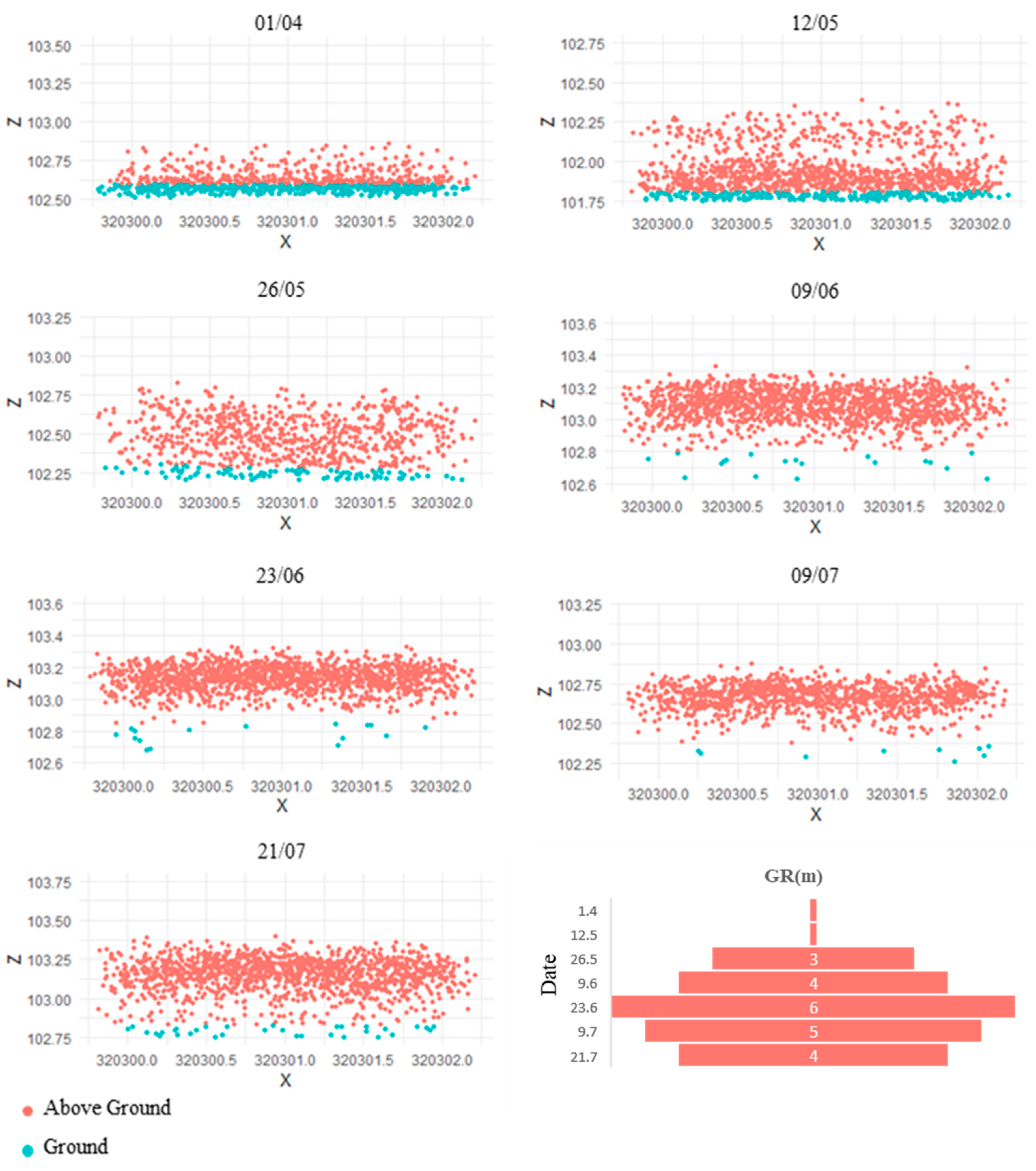
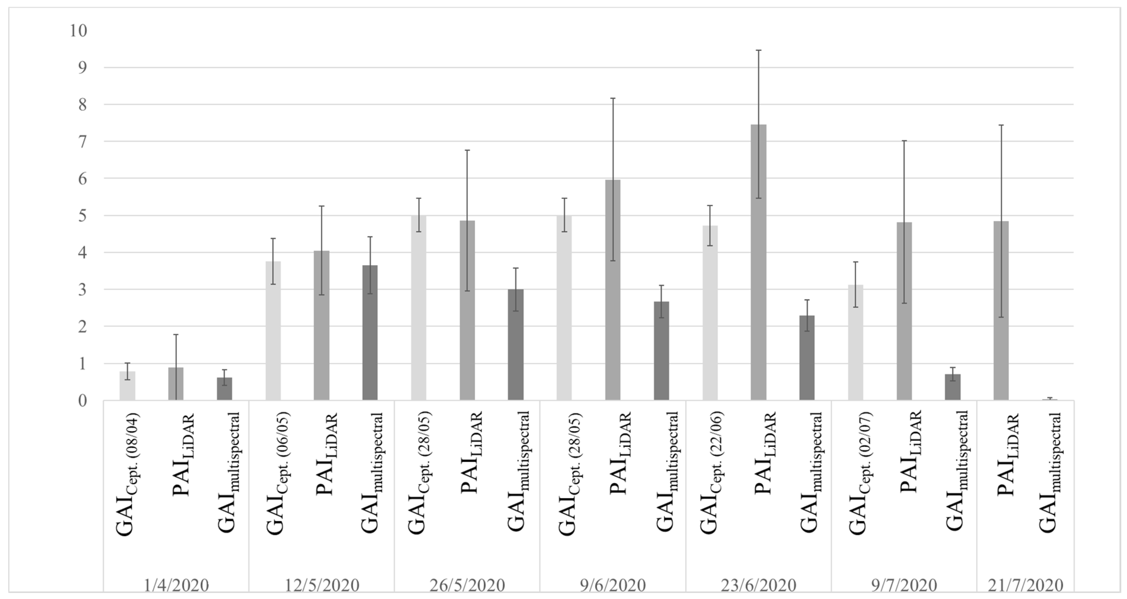
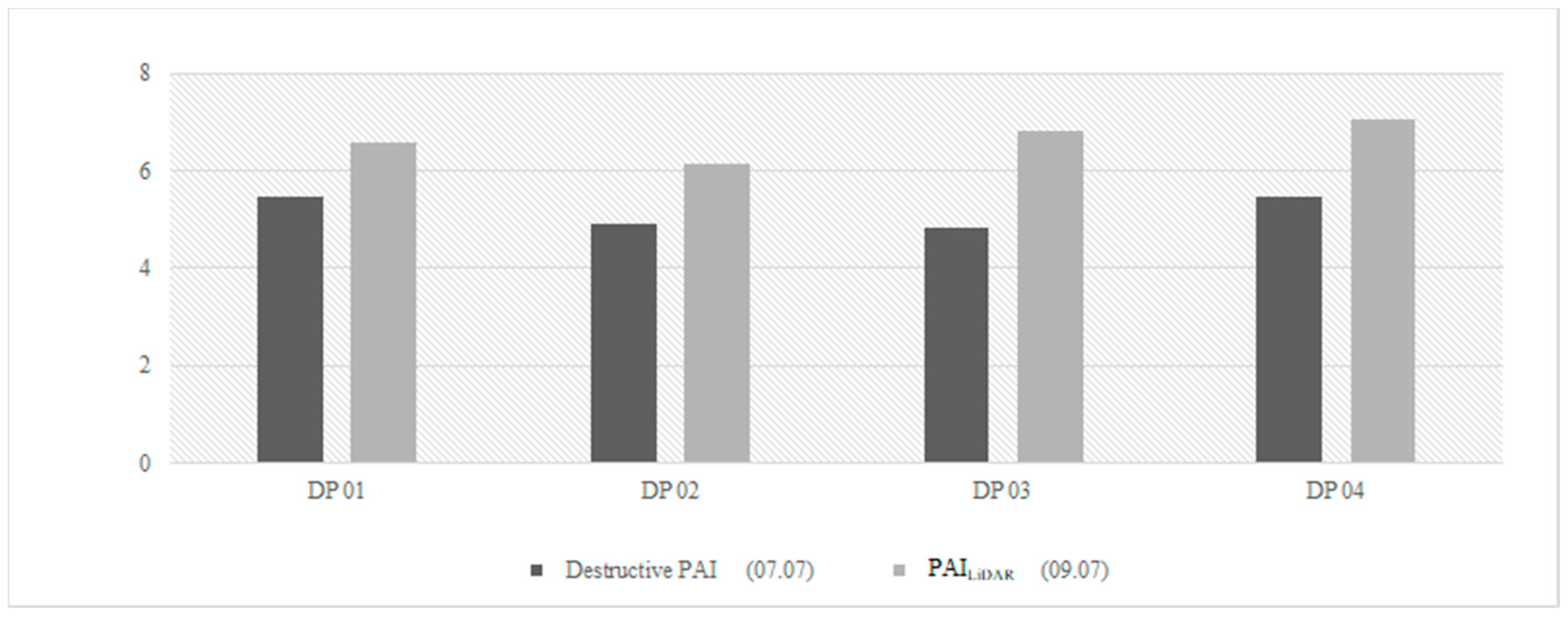
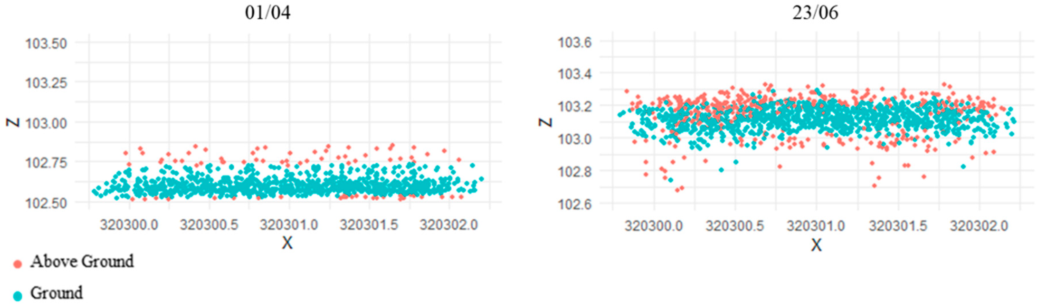
3.1. Comparison against Ground Measurements

The individual Sunscan SS1 ceptometer ground GAI measurements for each of the designated plot areas (CPs, see Figure 2) were averaged together and compared against the mean values of PAI_LiDAR and GAI_{multispectral} over the ground measurement plots for each date, consisting of approximately 9600 pixels. The ceptometer collections took place on different days to the aerial acquisitions but were grouped based on temporal proximity. The results of this comparison are represented in Figure 5. All three methods show similar results for the first two dates. The GAI_{multispectral} values continuously decrease after the 12th of May, while the PAI_LiDAR estimates increase to reach a maximum on the 9th of July. The ceptometer and LiDAR results remain close in April to early June, with a difference of 3–18%, but the differences in the estimations grow to approximately 50–58% after late June for each date.

The destructive PAI measurement plot (DP, see Figure 2) mean values were compared to the mean PAI_LiDAR values of adjacent plots of approximately 5.4 m² consisting of 200 pixels each. Values from the PAI_LiDAR data were taken from an adjacent area to the DPs (see Figure 2) because the closest flight campaign was just after the DP collection. The next closest date was two weeks prior. The results (see Figure 6) show that the values with the LiDAR methods are 28% larger at this period in the growing season.

The GAI ceptomoter measurements were used to determine a R² = 0.45 and a RMSE = 2.05 for the GAI_{multispectral} when using a k(θ) from the literature. For PAI_LiDAR, the first three ceptometer measurements were used (08/04–28/05). This was the period in the growing season when there was little to no senescence, especially near the center of the field. It was assumed that PAI and GAI were the same during this period and at those CP locations. Then, the PAI calculated for each DP area from destructive measurements was used for comparison to the 09/07 data. A R² = 0.89 and a RMSE = 0.87 were determined for the PAI_LiDAR results when also using a k(θ) from the literature.

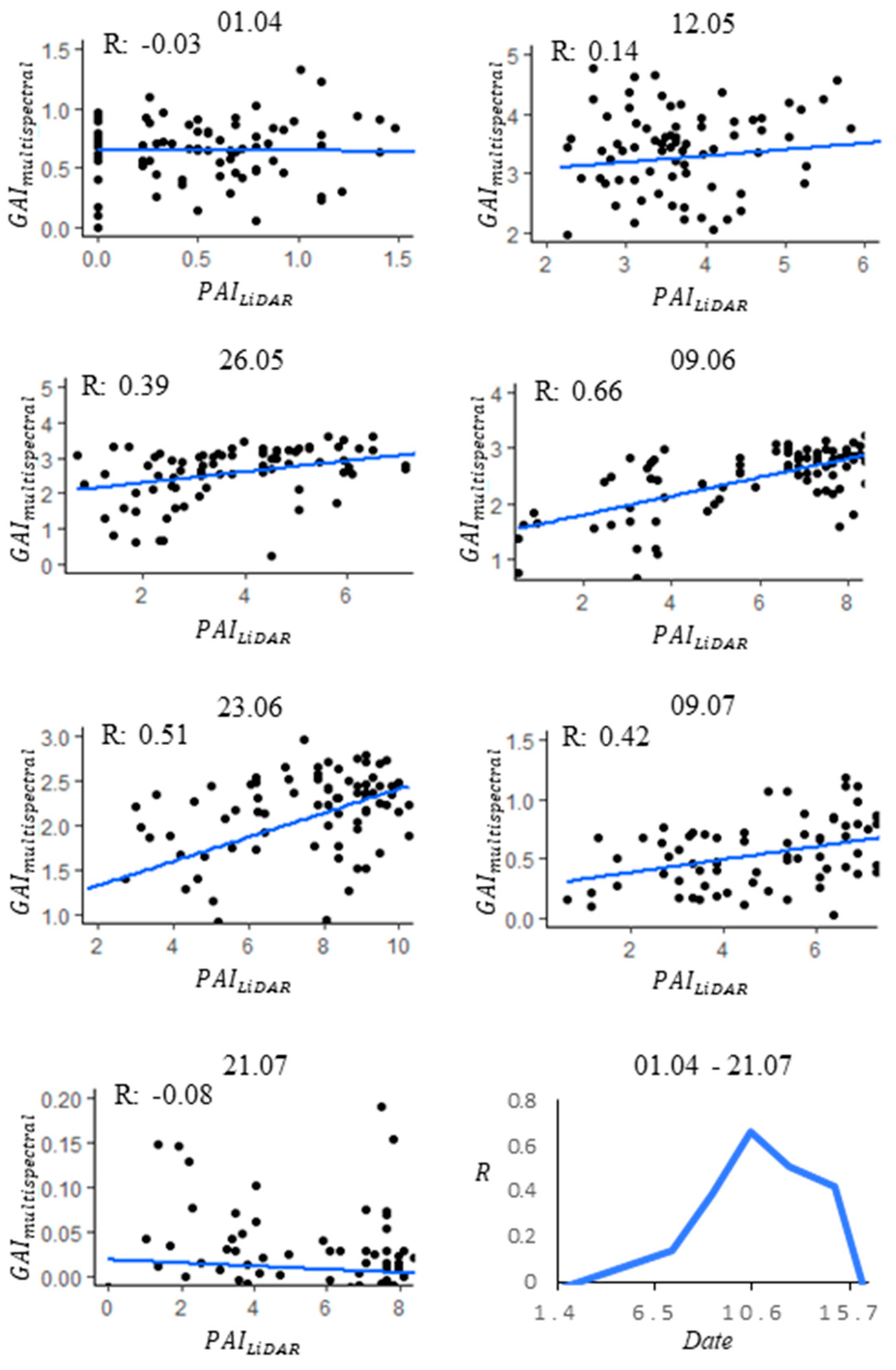
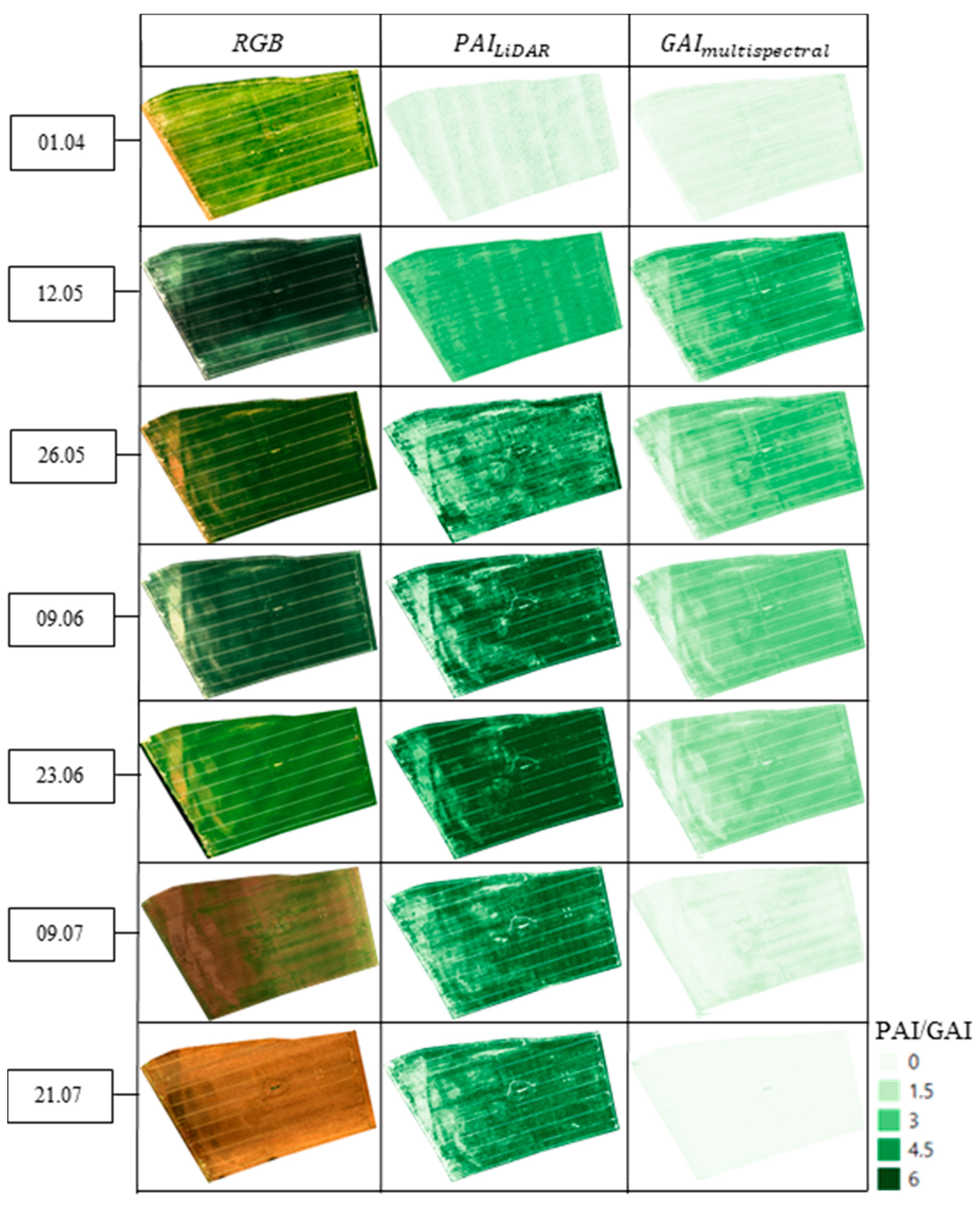
3.2. Spatial Variation in Values

In order to evaluate the relationships between the LiDAR and multispectral methods, spatial sampling was performed for each individual date using 82 evenly distributed points with the same point locations across all dates and methods (see Figure 7). As the passive optical methods using VIs derived from multispectral data are proven in past studies, they are used here to assess the LiDAR’s ability to detect the spatial variation in the canopy structure. There is not a significant correlation between early and late stages in the growing season, which can be attributed to optical NDVI’s dependence on plant pigment and the soil contribution to the signal, whilst LiDAR depends more on the entire canopy and its structure. The correlations are moderate to high (R = 0.39–0.66) mid-growing season. Although the magnitude of the absolute values is different, explained by the different plant elements sensed by the two methods, the relative spatial variation shows some consistency between the methods.

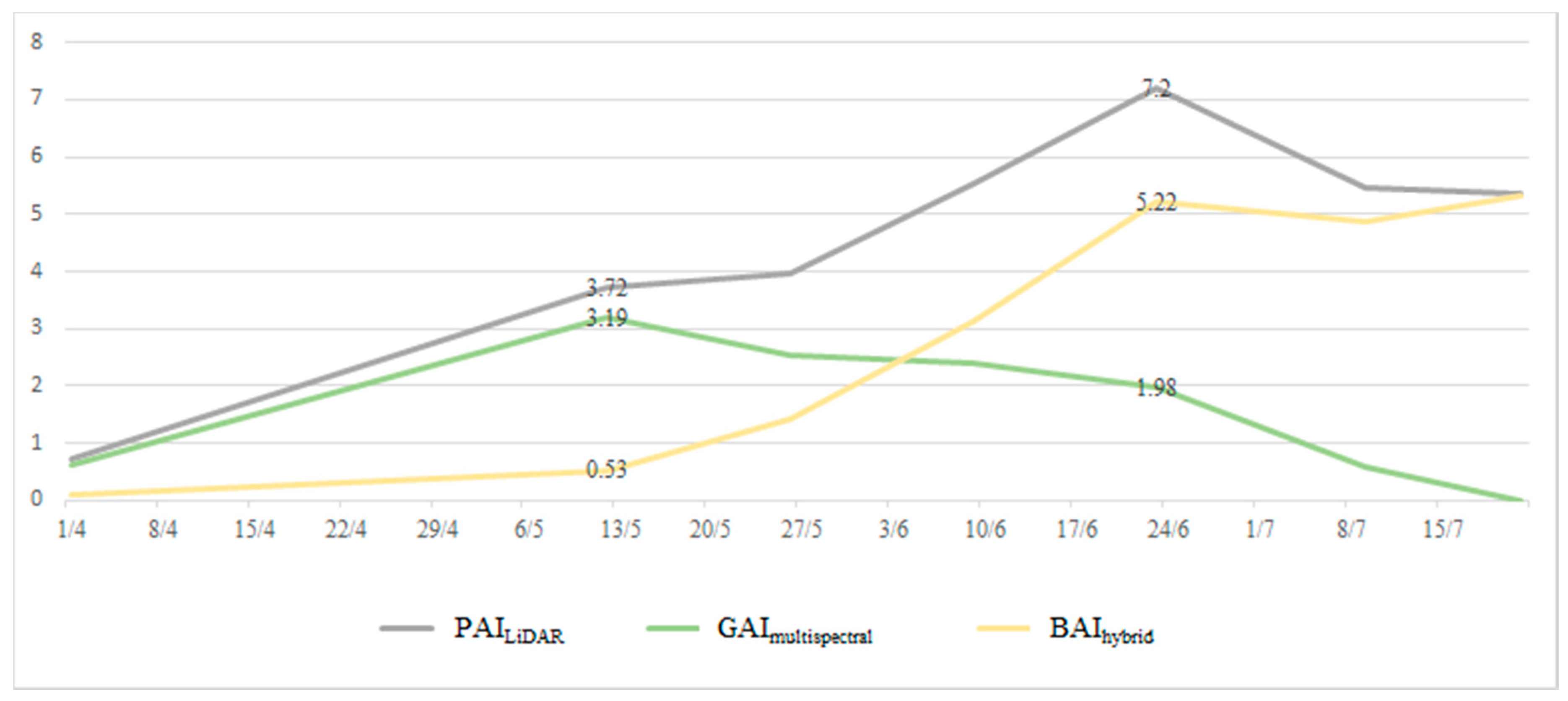
3.3. PAI, GAI, and BAI

The visualization of the results is presented in Figure 8, where the LiDAR and the multispectral results can be compared against the RGB imagery. Spatial heterogeneity among the crop is clearly visible in the RGB imagery, along with senescence starting on the western side of the field as early as late May. It can be seen that the LiDAR methodology used is able to capture these changes in crop structure within its PAI_LiDAR estimations. The GAI_{multispectral} calculated using passive optical means with NDVI exhibits similar patterns but the reflectance from the crop dissipates as the crop approaches the full senescence stage, as confirmed in the RGB imagery.

The temporal evolution of the field average of PAI_LiDAR and GAI_{multispectral} is depicted in Figure 9, where it can be seen how these two types of metrics and methods can complement one another when monitoring winter wheat. Both PAI and GAI are similar until 12 May 2020, before the appearance of senescence. This allows for the LiDAR and multispectral methods to be compared during this period in the growing season. The separation in values coincides with a dry period, as can be seen from the weather data in Figure A2. GAI_{multispectral} decreases after 12/5 and appears to level off towards the end of May with increased precipitation while PAI_LiDAR continues to increase. This also agrees with the results captured by the LiDAR crop height measurements seen in Figure 10. PAI_LiDAR decreases at the end of June but the GAI_{multispectral} decrease is more drastic when the crop enters senescence stages for the entire field.

This highlights the potential to distinguish between the PAI with reference to the complete aboveground biomass with LiDAR, the GAI for plant pigment with multispectral methods, and the non-green biomass with BAI as a byproduct of the combination of both methods.

4. Discussion and Future Directions for Improvement

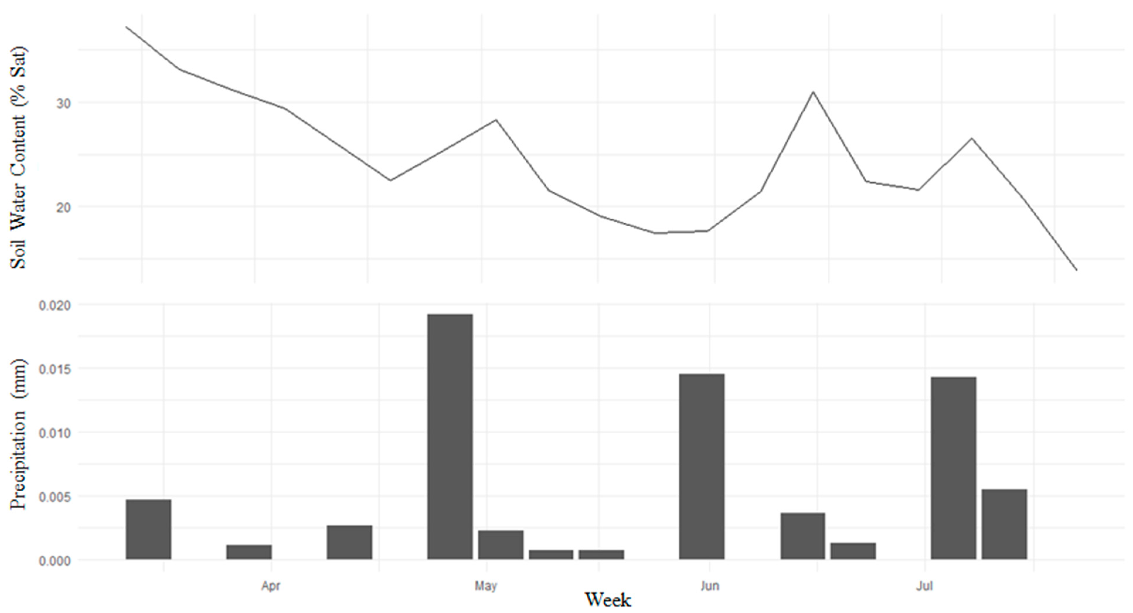
4.1. Time-Series Trend

The results of this study show that estimating canopy structure with LiDAR for crops such as winter wheat is feasible and may indeed have potential benefits. The differences in temporal evolutions of LiDAR and multispectral data are in agreement with expected values as they measure different parts of the vegetation. The PAI_LiDAR and GAI_{multispectral} are similar at the start of the growing season (1.4.2020–12.5.2020) as most plant elements are green at this time. The field GAI_{multispectral} decreases on 26.5.2020, which is due to an increase in plant stress and visible browning that begins to occur on the western part of the field. The precipitation and soil moisture data seen in Figure A2 show that precipitation had decreased in May, which possibly explains this sudden drop in GAI. PAI increase also slows down in this temporal window. The structures appearing on the western side are consistent with those soil areas with increased sand and gravel fractions closer to the surface, which are known to be more affected by water scarcity [47]. These patterns are also similar to those experienced with the previous TLS study for crop height at the same field during the 2008 and 2009 growing seasons [48]. Once prominent precipitation amounts appeared at the end of May and beginning of June, GAI decline slowed and PAI increase became steeper. The PAI_LiDAR field averages increased along with the increase in crop height (see Figure 10) during the growing season, as expected [29]. Values of PAI and GAI continued to separate throughout the growing season as winter wheat approached full senescence, with lower greenness in plant tissue and lower GAI values. However, PAI remained high, with LiDAR still being able to sense the variations in canopy density.

The PAI_LiDAR and the ground-ceptometer-derived GAI values are similar as there is little difference between GAI and PAI when the plant structure is mostly green [3]. Differences begin to occur as the field approaches senescence. The differences in values may be further exaggerated as effects such as clumping can cause underestimations in ground measurements and LiDAR-derived values are known to be overestimated when canopy density is at its highest. As seen in Figure 3, at the peak of crop growth, the point cloud consists mostly within the top portion of the crop with few signals passing through. This leads to a lack of differentiation throughout the crop and to less information about its structure. This low gap probability and loss of information could be linked to an overestimation of PAI_LiDAR in parts of the field. This possible overestimation may be suggested from the comparison made with the destructive PAI measurements. Inadequate collection parameters (i.e., flight profile, overlap, scan angle) could be the cause, failing to fully exploit the canopy gaps so that an appropriate characterization of the canopy density could be obtained.

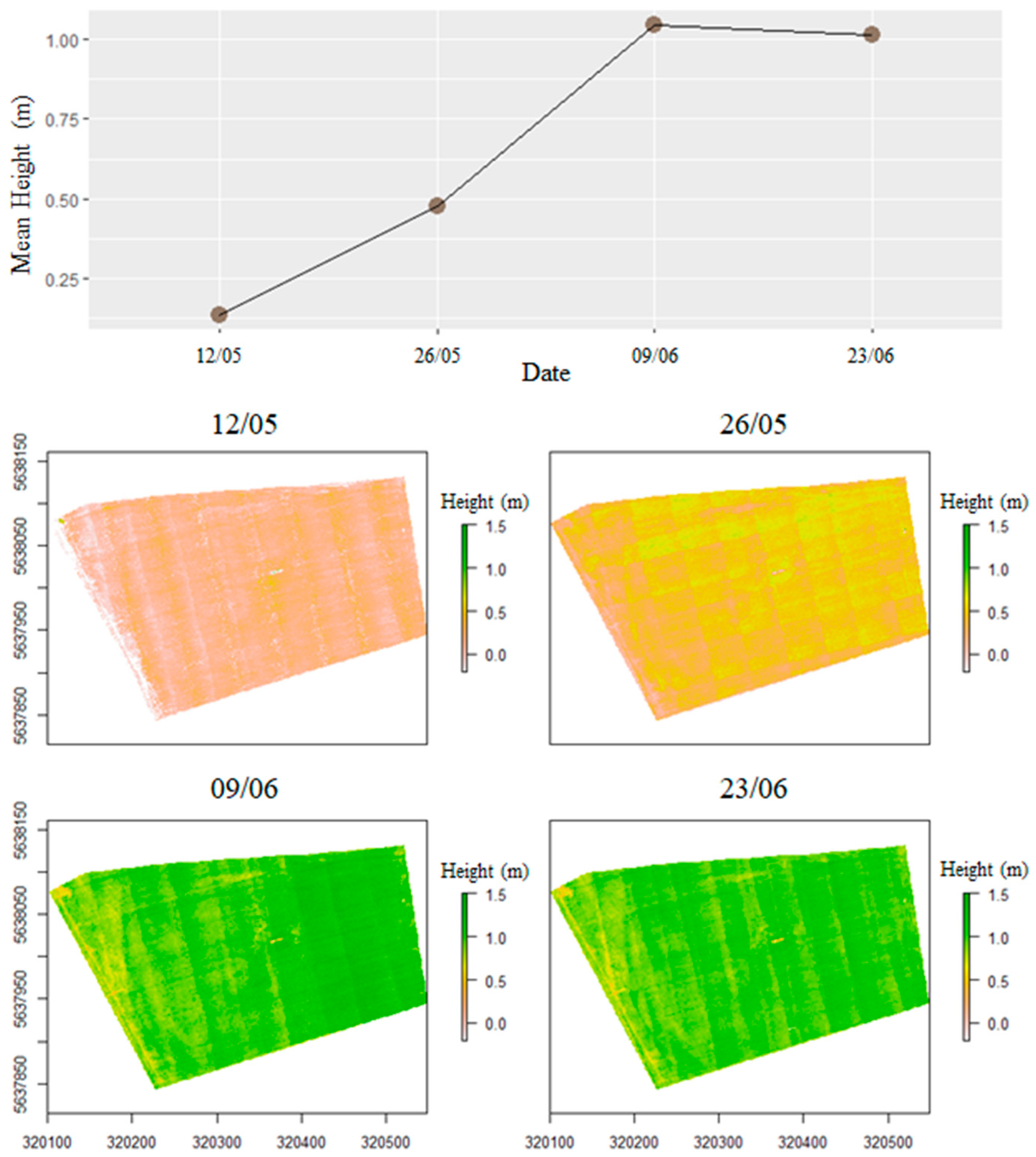
4.2. PAI_LiDAR Spatial Variation

The spatial variation in PAI_LiDAR correlates well with the GAI_{multispectral} estimates obtained from an already established method with passive optical sensors. The lack of correlations in the beginning and end of the growing season is likely due to the fact that the two methods sense different plant parts. The multispectral method is based on differences in spectral reflectance and therefore sensitive to plant pigments, while the LiDAR method is based on the sensor’s laser penetration through the whole canopy and thus affected by canopy density and gap probability. For example, when the crop reached complete senescence before harvest, the reflectance was essentially uniform at approximately the same values of bare soil, as all of the crop consisted of non-green senescent vegetation. However, unlike the multispectral approach, the LiDAR was able to detect the senescent vegetation. Although their spatial variation did not correlate on the first two dates and the last date, they provided similar spatial patterns in the mid-growing season.

4.3. Impacts of the Extinction Coefficient k(θ)

PAI_LiDAR benefited more than the GAI_{multispectral} from the k(θ) value selection based on the literature and was able to deliver estimations with a respectable ${\mathrm{R}}^2$ and RMSE. The k(θ) for LiDAR may not always agree well with those derived from other sensors. For example, in the study by Solberg et al. (2006) [57], an approximate k(θ) value of 0.7 was derived using ALS while the ground-based measurements were 0.51 and 0.44. The k(θ) could be a contributing factor to the PAI_LiDAR results overestimating at the height of the growing season. LiDAR resembles beam radiation that is more concentrated while the k(θ) was derived from direct and diffuse radiation as used in passive optical methods [32]. This can be better understood and improved by further analysis with various LiDAR collection parameters in comparison with k(θ) values derived from other sensors and with different crops.

Instead of using literature values, we evaluated the potential of a k(θ) calibration to characterize its general nature during changing crop conditions. The PAI_LiDAR and GAI_{multispectral} k(θ) were inversely calibrated using the ground measurements. The resulting PAI_LiDAR obtained a ${\mathrm{R}}^2$ = 0.91 and a RMSE = 0.43, whereas the GAI_{multispectral} obtained a R² = 0.96 and a RMSE = 0.31. The retrieved k(θ) values are listed in

Table 1. k(θ) values used for each date and method.

Date	GAImultispectral k(θ)	PAILiDAR k(θ)
1/4	0.47	0.37
12/5	0.34	0.37
26/5	0.22	0.35
9/6	0.19	0.4
23/6	0.17	0.4
9/7	0.09	0.45
21/7	0.09	0.45

. The GAI_{multispectral} k(θ) values changed with time and progressively declined throughout the growing season. The GAI_{multispectral} method incorporated for UAS for this project may benefit from a linearity adjustment factor in the equations for better results or studies without in situ measurements. The PAI_LiDAR appears to be more stable over time and shows promise that fixing this parameter would introduce just minor uncertainty, so that it could be incorporated using values from the literature [47,56]. It is worth noting that none of the ground measurements were taken on the same day as flight campaigns, but within a maximum time span of nine days. More specific reference measurements are needed for better interpretation.

4.4. Future Insights

There are several possible improvements that can be made to increase the accuracy and detail of results for future studies. Changes and balances between flight direction, scan angle, and overlap during data acquisition can be made to change the perspectives to create better information about the plant structure while increasing the chances of the LiDAR signal detecting gaps in the canopy [32]. The closer the flight lines are to one another, the higher the number of perspectives will be from the LiDAR with respect to the chosen scan angle. Implementing crosshatch flight paths could also increase accuracy by not only increasing overlap, but by increasing oblique perspectives from additional directions. These methods must be investigated and balanced with flight time and battery efficiency, for at a certain point, the improvements in accuracy may not be worth the prolonged acquisition duration. Off-nadir scan angles also help in finding gaps and understanding the canopy structure but have to be limited at an optimal point considering signal travel and strength. In the study by Morsdorf et al. (2006) [31], it is suggested that parameters such as laser wavelength and flying altitude affect LiDAR footprint size and point spacing, which influences accuracy and should be investigated further. Aside from flight parameters during the acquisition of the data, improvements can be made during the processing and calculation stages of the data. Studies have used other methods of analysis, including laser penetration index (LPI) and signal intensity, to characterize canopy structure [33]. Additionally, advancements in hardware provide further potential, such as with multi-frequency and multi-channel LiDAR systems. In future studies, combining additional variables or considerations within the analysis and flight parameterization has promise for improved estimations.

Considering that LiDAR provides a better characterization of the crop canopy structure, combining the LiDAR height and PAI_LiDAR values may give better estimates of biomass than previously seen with multispectral and photogrammetry methods [2]. GAI of winter wheat could also be calculated using the intensity of the LiDAR returns since the signal is emitted close to NIR [6]. The more products that this sensor can calculate without supporting data from other sensors and as a standalone sensor, the more efficient it becomes. For further consideration in its future potential, LiDAR is less affected by its environment, such as with solar zenith angles and cloudiness, as compared to UAS with passive sensors. LiDAR systems have already made huge leaps in size and as the market competition increases, the pricing will decline and the data processing will become more user-friendly, making these systems and potential methods more accessible for use in farm management [10].

5. Conclusions

A method to differentiate PAI, GAI, and BAI by UAS-mounted active (LiDAR) and passive (multispectral) sensors has been developed for a winter wheat case. Having the ability to differentiate between these products can improve the understanding of crop performance and carbon budget, which can increase the precision of farming practices. Additionally, proof of concept has been applied when calculating metrics for crop structure, such as PAI, with UAS-mounted LiDAR. It shows promise as it can replicate the structural patterns within the crop canopy, which is consistent with multispectral methods. The PAI_LiDAR and GAI_{multispectral} estimations were comparable before the appearance of senescence, providing further evidence in support of the methods tested. The LiDAR method is in agreement with other accepted non-destructive and destructive methods. It has been shown that this method may also be able to enhance or capture what might be missed with GAI_{multispectral} estimations, especially in the case of cereal crops. Without dependence on spectral reflectance and solar radiation, the LiDAR methods provide improved options for characterizing full crop canopy structure.

When LiDAR is used with a UAS, it provides further versatility in potential flight collection parameters as traditional ALS methods may be more restricted when it comes to lower flight altitudes and flight paths. There are still additional factors concerning flight planning, processing, and variables within the analysis to explore in order to further understand and increase the accuracy and feasibility of the methods presented. The flight parameters chosen in this study may not have fully exploited the canopy gaps when the crop was at its highest density, causing potential overestimation in values late in the growing season. Although improvements are possible, this study succeeds in providing evidence that UAS-mounted active and passive sensors can indeed be used to characterize the full canopy of crops such as winter wheat and differentiate between PAI, GAI, and BAI.

References

1. Yan, G.; Hu, R.; Luo, J.; Weiss, M.; Jiang, H.; Mu, X.; Xie, D.; Zhang, W. Review of indirect optical measurements of leaf area index: Recent advances, challenges, and perspectives. Agric. For. Meteorol. 2019, 265, 390–411. [Google Scholar] [CrossRef]
2. Zheng, G.; Moskal, L.M. Retrieving Leaf Area Index (LAI) using remote sensing: Theories, methods and sensors. Sensors 2009, 9, 2719–2745. [Google Scholar] [CrossRef] [PubMed] [Green Version]
3. Fang, H.; Baret, F.; Plummer, S.; Schaepman-Strub, G. An overview of global Leaf Area Index (LAI): Methods, products, validation, and applications. Rev. Geophys. 2019, 57, 739–799. [Google Scholar] [CrossRef]
4. Pasqualotto, N.; Delegido, J.; Van Wittenberghe, S.; Rinaldi, M.; Moreno, J. Multi-crop green LAI estimation with a new simple Sentinel-2 LAI Index (SeLI). Sensors 2019, 19, 904. [Google Scholar] [CrossRef] [PubMed] [Green Version]
5. Delegido, J.; Verrelst, J.; Rivera, J.P.; Ruiz-Verdú, A.; Moreno, J. Brown and green LAI mapping through spectral indices. Int. J. Appl. Earth Obs. Geoinformation 2015, 35(Part B), 350–358. [Google Scholar] [CrossRef]
6. Liu, S.; Baret, F.; Abichou, M.; Boudon, F.; Thomas, S.; Zhao, K.; Fournier, C.; Andrieu, B.; Irfan, K.; Hemmerlé, M.; et al. Estimating wheat green area index from ground-based LiDAR measurement using a 3D canopy structure model. Agric. For. Meteorol. 2017, 247, 12–20. [Google Scholar] [CrossRef]
7. Stark, B.; Zhao, T.; Chen, Y. An analysis of the effect of the bidirectional reflectance distribution function on remote sensing imagery accuracy from Small Unmanned Aircraft Systems. In Proceedings of the 2016 International Conference on Unmanned Aircraft Systems (ICUAS), IEEE, Arlington, VA, USA, 7–10 June 2016; pp. 1342–1350. [Google Scholar]
8. Baret, F.; de Solan, B.; Lopez-Lozano, R.; Ma, K.; Weiss, M. GAI Estimates of row crops from downward looking digital photos taken perpendicular to rows at 57.5° zenith angle: Theoretical considerations based on 3D architecture models and application to wheat crops. Agric. For. Meteorol. 2010, 150, 1393–1401. [Google Scholar] [CrossRef]
9. Kokaly, R.F.; Asner, G.P.; Ollinger, S.V.; Martin, M.E.; Wessman, C.A. Characterizing canopy biochemistry from imaging spectroscopy and its application to ecosystem studies. Remote Sens. Environ. 2009, 113, S78–S91. [Google Scholar] [CrossRef]
10. Bakuła, K.; Salach, A.; Wziątek, D.Z.; Ostrowski, W.; Górski, K.; Kurczyński, Z. Evaluation of the accuracy of lidar data acquired using a UAS for levee monitoring: Preliminary results. Int. J. Remote. Sens. 2017, 38, 2921–2937. [Google Scholar] [CrossRef]
11. Leblanc, S.G.; Chen, J.M.; Fernandes, R.; Deering, D.W.; Conley, A. Methodology comparison for canopy structure parameters extraction from digital hemispherical photography in boreal forests. Agric. For. Meteorol. 2005, 129, 187–207. [Google Scholar] [CrossRef] [Green Version]
12. Van Gardingen, P.; Jackson, G.; Hernandez-Daumas, S.; Russell, G.; Sharp, L. Leaf Area Index estimates obtained for clumped canopies using hemispherical photography. Agric. For. Meteorol. 1999, 94, 243–257. [Google Scholar] [CrossRef]
13. Ariza-Carricondo, C.; Di Mauro, F.; De Beeck, M.O.; Roland, M.; Gielen, B.; Vitale, D.; Ceulemans, R.; Papale, D. A comparison of different methods for assessing leaf area index in four canopy types. Cent. Eur. For. J. 2019, 65, 67–80. [Google Scholar] [CrossRef] [Green Version]
14. Welles, J.M.; Cohen, S. Canopy structure measurement by gap fraction analysis using commercial instrumentation. J. Exp. Bot. 1996, 47, 1335–1342. [Google Scholar] [CrossRef]
15. Broadhead, J.; Muxworthy, A.; Ong, C.; Black, C. Comparison of methods for determining leaf area in tree rows. Agric. For. Meteorol. 2003, 115, 151–161. [Google Scholar] [CrossRef] [Green Version]
16. Kalacska, M.; Calvo-Alvarado, J.C.; Sanchez-Azofeifa, G.A. Calibration and assessment of seasonal changes in leaf area index of a tropical dry forest in different stages of succession. Tree Physiol. 2005, 25, 733–744. [Google Scholar] [CrossRef] [PubMed] [Green Version]
17. Olivas, P.C.; Oberbauer, S.F.; Clark, D.B.; Clark, D.A.; Ryan, M.G.; O’Brien, J.J.; Ordoñez, H. Comparison of direct and indirect methods for assessing Leaf Area Index across a tropical rain forest landscape. Agric. For. Meteorol. 2013, 177, 110–116. [Google Scholar] [CrossRef]
18. Kobayashi, H.; Ryu, Y.; Baldocchi, D.D.; Welles, J.M.; Norman, J.M. On the correct estimation of gap fraction: How to remove scattered radiation in gap fraction measurements? Agric. For. Meteorol. 2013, 174–175, 170–183. [Google Scholar] [CrossRef]
19. Weiss, M.; Baret, F.; Smith, G.; Jonckheere, I.; Coppin, P. Review of methods for in situ leaf area index (LAI) determination. Agric. For. Meteorol. 2004, 121, 37–53. [Google Scholar] [CrossRef]
20. Fang, H.; Li, W.; Wei, S.; Jiang, C. Seasonal variation of leaf area index (LAI) over paddy rice fields in NE China: Intercomparison of destructive sampling, LAI-2200, digital hemispherical photography (DHP), and AccuPAR methods. Agric. For. Meteorol. 2014, 198–199, 126–141. [Google Scholar] [CrossRef]
21. Martinez, B.; García-Haro, F.; Camacho de Coca, F. Derivation of high-resolution leaf area index maps in support of validation activities: Application to the cropland Barrax site. Agric. For. Meteorol. 2009, 149, 130–145. [Google Scholar] [CrossRef]
22. Richardson, A.D.; Dail, D.B.; Hollinger, D. Leaf Area Index uncertainty estimates for model–data fusion applications. Agric. For. Meteorol. 2011, 151, 1287–1292. [Google Scholar] [CrossRef]
23. Verger, A.; Martínez, B.; Coca, F.C.; García-Haro, F.J. Accuracy assessment of fraction of vegetation cover and leaf area index estimates from pragmatic methods in a cropland area. Int. J. Remote Sens. 2009, 30, 2685–2704. [Google Scholar] [CrossRef]
24. Woodgate, W.; Jones, S.D.; Suarez, L.; Hill, M.J.; Armston, J.D.; Wilkes, P.; Soto-Berelov, M.; Haywood, A.; Mellor, A. Understanding the variability in ground-based methods for retrieving canopy openness, gap fraction, and leaf area index in diverse forest systems. Agric. For. Meteorol. 2015, 205, 83–95. [Google Scholar] [CrossRef]
25. Chiroro, D.; Armston, J.; Makuvaro, V. An investigation on the utility of the Sunscan ceptometer in estimating the leaf area index of a sugarcane canopy. Proc. South Afr. Technol. Assoc. 2006, 80, 143. [Google Scholar]
26. Dhami, H.; Yu, K.; Xu, T.; Zhu, Q.; Dhakal, K.; Friel, J.; Li, S.; Tokekar, P. Crop height and plot estimation from unmanned aerial vehicles using 3D LiDAR. arXiv 2020, arXiv:1910.14031. [Google Scholar]
27. Neuville, R.; Bates, J.S.; Jonard, F. Estimating forest structure from UAV-mounted LiDAR point cloud using machine learning. Remote. Sens. 2021, 13, 352. [Google Scholar] [CrossRef]
28. Meng, X.; Shang, N.; Zhang, X.; Li, C.; Zhao, K.; Qiu, X.; Weeks, E. Photogrammetric UAV Mapping of Terrain under Dense Coastal Vegetation: An object-oriented classification ensemble algorithm for classification and terrain correction. Remote. Sens. 2017, 9, 1187. [Google Scholar] [CrossRef] [Green Version]
29. Huang, Z.; Zou, Y. Inversion of Forest Leaf Area Index based on Lidar data. TELKOMNIKA Telecommun. Comput. Electron. Control. 2016, 14, 44. [Google Scholar] [CrossRef] [Green Version]
30. Korhonen, L.; Korpela, I.; Heiskanen, J.; Maltamo, M. Airborne discrete-return LIDAR data in the estimation of vertical canopy cover, angular canopy closure and leaf area index. Remote. Sens. Environ. 2011, 115, 1065–1080. [Google Scholar] [CrossRef]
31. Morsdorf, F.; Kötz, B.; Meier, E.; Itten, K.; Allgöwer, B. Estimation of LAI and fractional cover from small footprint airborne laser scanning data based on gap fraction. Remote. Sens. Environ. 2006, 104, 50–61. [Google Scholar] [CrossRef]
32. Richardson, J.J.; Moskal, L.M.; Kim, S.-H. Modeling approaches to estimate effective leaf area index from aerial discrete-return LIDAR. Agric. For. Meteorol. 2009, 149, 1152–1160. [Google Scholar] [CrossRef]
33. Sabol, J.; Patočka, Z.; Mikita, T. Usage of Lidar Data for Leaf Area Index estimation. Geosci. Eng. 2014, 60, 10–18. [Google Scholar] [CrossRef] [Green Version]
34. Sasaki, T.; Imanishi, J.; Ioki, K.; Song, Y.; Morimoto, Y. Estimation of leaf area index and gap fraction in two broad-leaved forests by using small-footprint airborne LiDAR. Landsc. Ecol. Eng. 2013, 12, 117–127. [Google Scholar] [CrossRef]
35. Rogers, S.R.; Manning, I.; Livingstone, W. Comparing the spatial accuracy of digital surface models from four unoccupied aerial systems: Photogrammetry versus LiDAR. Remote. Sens. 2020, 12, 2806. [Google Scholar] [CrossRef]
36. Becirevic, D.; Klingbeil, L.; Honecker, A.; Schumann, H.; Rascher, U.; Léon, J.; Kuhlmann, H. On the derivation of crop heights from multitemporal UAV based imagery. ISPRS Ann. Photogramm. Remote. Sens. Spat. Inf. Sci. 2019, 95–102. [Google Scholar] [CrossRef] [Green Version]
37. Cao, L.; Liu, H.; Fu, X.; Zhang, Z.; Shen, X.; Ruan, H. Comparison of UAV LiDAR and digital aerial photogrammetry point clouds for estimating forest structural attributes in subtropical planted forests. Forests 2019, 10, 145. [Google Scholar] [CrossRef] [Green Version]
38. Davidson, L.; Mills, J.P.; Haynes, I.; Augarde, C.; Bryan, P.; Douglas, M. Airborne to UAS LiDAR: An analysis of UAS LiDAR ground control targets. ISPRS Int. Arch. Photogramm. Remote. Sens. Spat. Inf. Sci. 2019, XLII-2/W13, 255–262. [Google Scholar] [CrossRef] [Green Version]
39. Bukowiecki, J.; Rose, T.; Ehlers, R.; Kage, H. High-throughput prediction of whole season green area index in winter wheat with an airborne multispectral sensor. Front. Plant Sci. 2020, 10, 10. [Google Scholar] [CrossRef]
40. Deery, D.M.; Rebetzke, G.J.; Jimenez-Berni, J.A.; Condon, A.G.; Smith, D.J.; Bechaz, K.M.; Bovill, W.D. Ground-Based LiDAR improves phenotypic repeatability of above-ground biomass and crop growth rate in wheat. Plant Phenomics 2020, 2020, 1–11. [Google Scholar] [CrossRef]
41. Wang, D.; Xin, X.; Shao, Q.; Brolly, M.; Zhu, Z.; Chen, J. Modeling aboveground biomass in hulunber grassland ecosystem by using unmanned aerial vehicle discrete lidar. Sensors 2017, 17, 180. [Google Scholar] [CrossRef] [Green Version]
42. Fu, Z.; Jindi, W.; Jinling, S.; Zhou, H.; Pang, Y.; Chen, B. Estimation of forest canopy leaf area index using MODIS, MISR, and LiDAR observations. J. Appl. Remote. Sens. 2011, 5, 53530. [Google Scholar] [CrossRef]
43. Hilker, T.; Wulder, M.A.; Coops, N.C. Update of forest inventory data with LIDAR and high spatial resolution satellite imagery. Can. J. Remote. Sens. 2008, 34, 5–12. [Google Scholar] [CrossRef]
44. Jensen, J.L.; Humes, K.S.; Vierling, L.A.; Hudak, A.T. Discrete return lidar-based prediction of leaf area index in two conifer forests. Remote. Sens. Environ. 2008, 112, 3947–3957. [Google Scholar] [CrossRef] [Green Version]
45. Ma, H.; Song, J.; Wang, J.; Xiao, Z.; Fu, Z. Improvement of spatially continuous forest LAI retrieval by integration of discrete airborne LiDAR and remote sensing multi-angle optical data. Agric. For. Meteorol. 2014, 60–70. [Google Scholar] [CrossRef]
46. Bogena, H.; Montzka, C.; Huisman, J.; Graf, A.; Schmidt, M.; Stockinger, M.; Von Hebel, C.; Hendricks-Franssen, H.; Van Der Kruk, J.; Tappe, W.; et al. The TERENO-Rur hydrological observatory: A multiscale multi-compartment research platform for the advancement of hydrological science. Vadose Zone J. 2018, 17, 180055. [Google Scholar] [CrossRef]
47. Brogi, C.; Huisman, J.A.; Herbst, M.; Weihermüller, L.; Klosterhalfen, A.; Montzka, C.; Reichenau, T.G.; Vereecken, H. Simulation of spatial variability in crop leaf area index and yield using agroecosystem modeling and geophysics-based quantitative soil information. Vadose Zone J. 2020, 19, e20009. [Google Scholar] [CrossRef] [Green Version]
48. Hoffmeister, D.; Waldhoff, G.; Korres, W.; Curdt, C.; Bareth, G. Crop height variability detection in a single field by multi-temporal terrestrial laser scanning. Precis. Agric. 2016, 17, 296–312. [Google Scholar] [CrossRef]
49. Gielen, B.; Acosta, M.; Altimir, N.; Buchmann, N.; Cescatti, A.; Ceschia, E.; Fleck, S.; Hörtnagl, L.; Klumpp, K.; Kolari, P.; et al. Ancillary vegetation measurements at ICOS ecosystem stations. Int. Agrophysics 2018, 32, 645–664. [Google Scholar] [CrossRef]
50. Chen, J.M.; Rich, P.M.; Gower, S.T.; Norman, J.M.; Plummer, S. Leaf area index of boreal forests: Theory, techniques, and measurements. J. Geophys. Res. Atmos. 1997, 102, 29429–29443. [Google Scholar] [CrossRef]
51. Zhang, W.; Qi, J.; Wan, P.; Wang, H.; Xie, D.; Wang, X.; Yan, G. An easy-to-use airborne LiDAR data filtering method based on cloth simulation. Remote. Sens. 2016, 8, 501. [Google Scholar] [CrossRef]
52. Ali, M.; Montzka, C.; Stadler, A.; Menz, G.; Thonfeld, F.; Vereecken, H. Estimation and validation of RapidEye-based time-series of leaf area index for winter wheat in the Rur Catchment (Germany). Remote Sens. 2015, 7, 2808–2831. [Google Scholar] [CrossRef] [Green Version]
53. Thorp, K.R.; Hunsaker, D.J.; French, A.N. Assimilating leaf area index estimates from remote sensing into the simulations of a cropping systems model. Trans. ASABE 2010, 53, 251–262. [Google Scholar] [CrossRef]
54. Ryu, J.-H.; Na, S.-I.; Cho, J. Inter-comparison of normalized difference vegetation index measured from different footprint sizes in cropland. Remote. Sens. 2020, 12, 2980. [Google Scholar] [CrossRef]
55. Khaliq, A.; Comba, L.; Biglia, A.; Ricauda Aimonino, D.; Chiaberge, M.; Gay, P. Comparison of satellite and UAV-based multispectral imagery for vineyard variability assessment. Remote. Sens. 2019, 11, 436. [Google Scholar] [CrossRef] [Green Version]
56. Tan, C.-W.; Zhang, P.-P.; Zhou, X.-X.; Wang, Z.-X.; Xu, Z.-Q.; Mao, W.; Li, W.-X.; Huo, Z.-Y.; Guo, W.-S.; Yun, F. Quantitative monitoring of leaf area index in wheat of different plant types by integrating NDVI and Beer-Lambert law. Sci. Rep. 2020, 10, 929. [Google Scholar] [CrossRef]
57. Solberg, S.; Næsset, E.; Hanssen, K.H.; Christiansen, E. Mapping defoliation during a severe insect attack on Scots pine using airborne laser scanning. Remote. Sens. Environ. 2006, 102, 364–376. [Google Scholar] [CrossRef]
Figure 1. (A) The DJI Matrice 600 used in the study with (B) the YellowScan Surveyor LiDAR mounted below. In addition, the (C) Micasense RedEdge-M multispectral sensor that was used on a separate DJI Matrice 600.
Remotesensing 13 00710 g001
Figure 2. Natural color composite of the field taken on 09.07.2020 with locations of the ground sampling. (A) shows the CP locations of the non-destructive measurements that were taken throughout the growing season with the ceptometer instrument and (B) shows the DP locations of the destructive measurements that were taken on 07.07.20. Note that the imagery was from later in the growing season and the brown coloring indicates those areas experiencing senescence.
Remotesensing 13 00710 g002
Figure 3. Cross-sections (2 m) of the LiDAR point clouds of each UAS acquisition date with the resulting segmentations visualized and the grid resolution (GR) values used.
Remotesensing 13 00710 g003
Figure 4. Sketch of the methodological approach used to calculate PAI from UAS-mounted LiDAR. The flight line distance (fld) is the distance between each parallel flight path and can determine the number of times and at what angles a particular area is viewed while also being related to point density in relation to the chosen scan angle. The point density (Pd) of the ground points is inversely related to the crop height as LiDAR signals are intercepted along the vertical axis of the crop canopy, ultimately affecting the Cloth Simulation Filtering (CSF) parameters used for segmentation.
Remotesensing 13 00710 g004
Figure 5. Comparison between the Sunscan SS1 ceptometer, the PAILiDAR, and the GAImultispectral estimations at each ground measurement plot location with a confidence interval of ~95%. The collection date is noted separately in the graph for the SS1 ceptometer (GAIcept) ground collections. Note that there is no ceptometer measurement for 21/7/2020 as 02/07/2020 was the last date on which a ceptometer measurement was taken in any of the CPs.
Remotesensing 13 00710 g005
Figure 6. Comparison of the destructive PAI measurements and the PAILiDAR averages taken with the same sample area size adjacent to the destructive plots.
Remotesensing 13 00710 g006
Figure 7. Spatial and temporal correlations between the LiDAR-derived PAI and the multispectral-derived GAI. Pearson correlation coefficients (R) are depicted for each measurement campaign during the growing season. Note that 82 evenly distributed points across both methods were used for each date.
Remotesensing 13 00710 g007
Figure 8. Time-series of PAI and GAI obtained with LiDAR and multispectral methods, respectively, and compared to RGB images.
Remotesensing 13 00710 g008
Figure 9. Temporal evolution of field average LiDAR-derived PAI and multispectral-derived GAI values. With the hybrid comparison of these two types of methods and products, the Brown Are Index (BAI) is estimated.
Remotesensing 13 00710 g009
Figure 10. Temporal (top) and spatial (bottom) variation in the average winter wheat height at the Selhausen ICOS field from UAS LiDAR. The heights were derived by subtracting the crop surface model (CSM) created for each date (12/05, 26/05, 09/06, 23/06) and having it subtracted by a digital terrain model (DTM) derived with the ground points from the UAS LiDAR data (01/04) at the beginning of the growing season. Note that a high scanning angle was used on the first collection (01/04) because of the large flight line spacing. The high scan angle decreased the point precision and number at the edges of the scan swath, causing noticeable lines when subtracted from the other data dates.
Remotesensing 13 00710 g010