Article

Refining Altimeter-Derived Gravity Anomaly Model from Shipborne Gravity by Multi-Layer Perceptron Neural Network: A Case in the South China Sea

1
College of Geodesy and Geomatics, Shandong University of Science and Technology, Qingdao 266590, China
2
Second Institute of Oceanography of MNR, Hangzhou 310012, China
3
Chinese Academy of Surveying and Mapping, Beijing 100036, China
*
Author to whom correspondence should be addressed.
Remote Sens. 2021, 13(4), 607; https://doi.org/10.3390/rs13040607
Submission received: 2 December 2020 / Revised: 30 January 2021 / Accepted: 4 February 2021 / Published: 8 February 2021
(This article belongs to the Special Issue Geodesy for Gravity and Height Systems)

Abstract

:
Shipborne gravity can be used to refine altimeter-derived gravity whose accuracy is low in shallow waters and areas with complex submarine topography. As altimeter-derived gravity only within a small radius around the shipborne data can be corrected by traditional methods, a new method based on multi-layer perceptron (MLP) neural network is proposed to refine the altimeter-derived gravity. Input variables of MLP include the positional information at observation points and geophysical information (from our own South China Sea gravity anomaly model (SCSGA) V1.0 and bathymetry model ETOPO1) at grid points around observation points. Output variables of MLP are the refined residual gravity anomalies at observation points. Training shipborne data are classified into four cases to train four MLP models, which are used to predict the refined gravity anomaly model SCSGA V1.1. Then all of the training shipborne data are used for training an MLP model to predict the refined gravity anomaly model SCSGA V1.2. Assessed by testing shipborne data, the accuracy of SCSGA V1.2 is 0.14 mGal higher than that of SCSGA V1.0, and similar to that of SCSGA V1.1. Compared with the original gravity anomaly model (SCSGA V1.0), the accuracy of the refined gravity anomaly model (SCSGA V1.2) by MLP is improved by 4.4% in areas where the training data are concentrated, and also improved by 2.2% in other areas. Therefore, the method of MLP can be used to refine the altimeter-derived gravity model by shipborne gravity, overcoming the problem of limited correction radius for traditional methods.

Graphical Abstract

1. Introduction

Precise ocean gravity models play an important role in geodetic and geophysical fields such as studying the Earth’s shape [1], interpreting lithospheric structure [2,3], exploiting marine resources [4], exploring space and improving aviation [5,6].
Abundant altimetric data have been collected since the 1970s and are homogenous over the oceans. Consequently, altimetric data play a major role in determining marine gravity models [7,8]. The global precision of gravity anomalies derived from multiple altimetry satellites whose ground track interval is about 2.5 km is 1~2 mGal (1 mGal is equal to 10−5 m/s2) [8,9]. Even so, the altimetry waveforms can be contaminated by land and reefs, so the accuracy of altimeter-derived gravity decreases with the increasing proximity to the coastline [10,11]. The standard deviation (STD) of altimeter-measured sea surface heights increases with decreasing water depth [10]. Meanwhile, water depth in coastal areas is shallow, so the precision of altimeter-derived gravity is low in shallow waters. Gravity anomalies are related to submarine topographic undulation and crustal density variations [12,13,14]. Gravity anomalies change dramatically in areas with large topographic undulation. As gravity anomalies are derived from altimetric data in a calculation windows (tens of kilometers), the precision of altimeter-derived gravity is lower in areas with notable submarine topography [15,16,17]. The precision of modern shipborne gravity with higher resolution is approximately 1~3 mGal [18]. Moreover, coastlines and submarine topography have less effects on the accuracy of shipborne gravity than altimeter-derived gravity.
Altimetric data and shipborne gravity are complementary sources of ocean gravity models [19]. First, altimetric data have the global coverage, and consequently supply gravity information in areas where there are few shipborne data. Second, shipborne gravity data are abundant in several regions of tectonic interest and contain a wealth of short-wavelength information [20]. Therefore, shipborne gravity can be used to improve the resolution of the marine gravity model and the precision of altimeter-derived gravity in shallow waters and areas with complex submarine topography.
There are two common methods to determine marine gravity from altimetric data and shipborne gravity. One is to directly calculate gravity anomalies by using shipborne gravity and altimetric data. The methods of least-squares collocation [21,22] and radial basis functions [23] are commonly applied to derive marine gravity, in which covariance matrices for shipborne gravity and altimetric data should be constructed. The precise covariance matrices are hard to be evaluated. The other is to refine altimeter-derived gravity anomalies by shipborne data based on the method of least-squares collocation [15]. The above methods are mainly based on the spatial relationship between shipborne and altimeter-derived data. Hence, compared with altimeter-derived gravity anomalies, the accuracy of gravity anomalies determined from shipborne and altimetric data is improved only in a small radius around shipborne observation points. Taking sparse and uneven distribution of shipborne data into account, a new method should be proposed to expand the correction area for altimeter-derived gravity models.
Machine learning is the subfield of computer science, giving computers the ability to learn the mapping from inputs to outputs without explicitly programming [24]. An advanced type of machine learning architecture employed by neural networks is deep learning, whose intent is to discover more abstract features in the higher levels of the representation. Therefore, the various features in data can be recognized from a small data set [25,26]. Multi-layer perceptron (MLP) neural network, a typical feedforward neural network, is widely applied to study fields of geology [27], meteorology [28,29] and energy science [30].
The South China Sea (SCS), the largest and deepest semi-enclosed sea area of China seas, has winding coastlines, abundant islands and complex submarine topography [31,32]. Hence, the SCS, covering 105° E–125° E and 0° N–30° N, is selected as the study region. As altimeter-derived gravity anomalies are related to submarine topography and its slopes, a method based on MLP neural network is proposed to improve the accuracy of altimeter-derived gravity by using shipborne data. The modern shipborne data in shallow waters and areas with large submarine topography slopes are used to train the relationship model among positions, altimeter-derived gravity anomalies, bathymetry, submarine topography slopes and shipborne gravity anomalies. Consequently, the model can be used to refine altimeter-derived gravity anomalies in shallow waters and areas with large submarine topography slopes.
Research data and methods are presented in Section 2. In Section 2.1, the research data are introduced, including the altimetric gravity, shipborne gravity and other data. The accuracy of shipborne and altimeter-derived gravity is also evaluated. In Section 2.2, research methods about MLP and the structure of MLP are represented in detail. MLP models are built by training data in Section 3. Moreover, refined gravity anomalies at grid points in shallow waters and areas with large submarine topography slopes are predicted by the MLP models, and validated by testing data. The roles of input variables of MLP in refining altimeter-derived gravity are analyzed in Section 3.3. In Section 4, we discuss the accuracy improvement of the gravity model in frequency domain. Finally, conclusions are drawn in Section 5.

2. Materials and Methods

2.1. Research Data

2.1.1. Reference Gravity Model and Topography Model

The remove-restore method is used to derive gravity from altimetric data and refine the gravity model by using shipborne gravity. As the Earth Gravitational Field Model 2008 (EGM2008) is the globally recognized gravitational field [33,34], EGM2008 up to degree 2160 is selected as the reference gravity model.
ETOPO1 [35] is a 1 arc-minute global relief model of Earth’s surface that integrates land topography and ocean bathymetry. ETOPO1 released by the National Oceanic and Atmospheric Administration in 2008 is established from shoreline, bathymetric, topographic and integrated bathymetric–topographic data. The data sets are obtained from several agencies, including Scripps Institution of Oceanography, the US National Centers for Environmental Information (NCEI), the Mediterranean Science Commission and the Japan Oceanographic Data Center.

2.1.2. Shipborne Gravity

The shipborne gravity data available in the SCS are provided by NCEI and the Ministry of Natural Resources of P. R. China (MNR), as shown in Figure 1. Long wavelength system errors for each cruise of shipborne gravity are corrected by a quadratic polynomial regression [21]. Pointwise differences between the adjusted shipborne data and the reference gravity model are calculated, and the point with the difference greater than triple STD of all the differences is discarded. The rejected rates for NCEI and MNR are approximately 2.2% and 0%, respectively. The STDs of crossover gravity discrepancies are 11.55 mGal and 6.07 mGal before and after the adjustment.
The accuracy of shipborne gravity is mainly affected by that of navigation. Due to the low accuracy of celestial navigation for shipborne gravity before 1967, the precision of shipborne gravity is as low as tens of mGal [36]. With application of GPS in navigation and positioning of shipborne observations, the accuracy of shipborne gravity has been improved. The precision of modern shipborne gravity with high resolution is approximately 1~3 mGal [18]. Therefore, the shipborne data after the adjustment are divided into two parts: data before 1990 and data since 1990.
The accuracy of the two parts is evaluated by using crossover gravity discrepancies, which is 4.41 mGal and 3.93 mGal, respectively. There are no crossovers between MNR cruises, so the crossover gravity discrepancies are determined from NCEI data which mainly including data on two cruises of MW9006 and MW9007 measured in 1990. Data on the two cruises account for 88.4% of NCEI data since 1990. The accuracy of MNR data is higher than that of NCEI data [37], so the accuracy of shipborne data since 1990 is considered as 3.93 mGal. As submarine topography slopes have an influence on the accuracy of shipborne gravity, STDs of shipborne data in areas with different submarine slopes are calculated from crossover gravity discrepancies and listed in Table 1.

2.1.3. Altimeter-Derived Gravity Anomaly Model

The altimetric gravity anomaly model around the South China Sea (SCSGA) V1.0 [37] on a 1’ × 1’ grid is used in this study. The model is established from sea surface heights (SSHs) of several geodetic missions (GMs) and exact repeat missions. GM data are from ERS-1, Jason-1, Jason-2, HY-2A, CryoSat-2 and SARAL–AltiKa, as listed in Table 2 [37]. In the area covering 114.5° E–116.5° E and 17.5° N–18.5° N, tracks of altimetric data used to construct SCSGA V1.0 are shown in Figure 2.
First, mean dynamic topography is removed from SSHs to calculate along-track geoid gradients. Deflections of the vertical are determined from along-track geoid gradients by the least-squares collocation method, and then used to derive gravity anomalies by the inverse Vening–Meinesz formula [38]. During the process, weights of geoid gradients from the Ka-band altimeter and the Ku-band altimeter for the least-squares collocation method are determined by different methods.
The accuracy of SCSGA V1.0 is 2.78 mGal in the SCS, which is slightly better than recognized global marine gravity models [7,8] released by the Technical University of Denmark and the Scripps Institution of Oceanography. The Philippine sea area with winding coastlines, abundant islands and larger submarine topography slopes has the lower gravity accuracy than other areas in the SCS. Therefore, SCSGA V1.0 is compared with shipborne gravity anomalies since 1990 in shallow waters (<100 m) as listed in Table 3 and in deep waters (>100 m) with different submarine topography slopes as listed in Table 4. As shallow areas are adjacent to land and islands, the results suggest that the accuracy of altimeter-derived gravity anomalies is affected by land, islands and submarine topography slopes.

2.2. Methodology

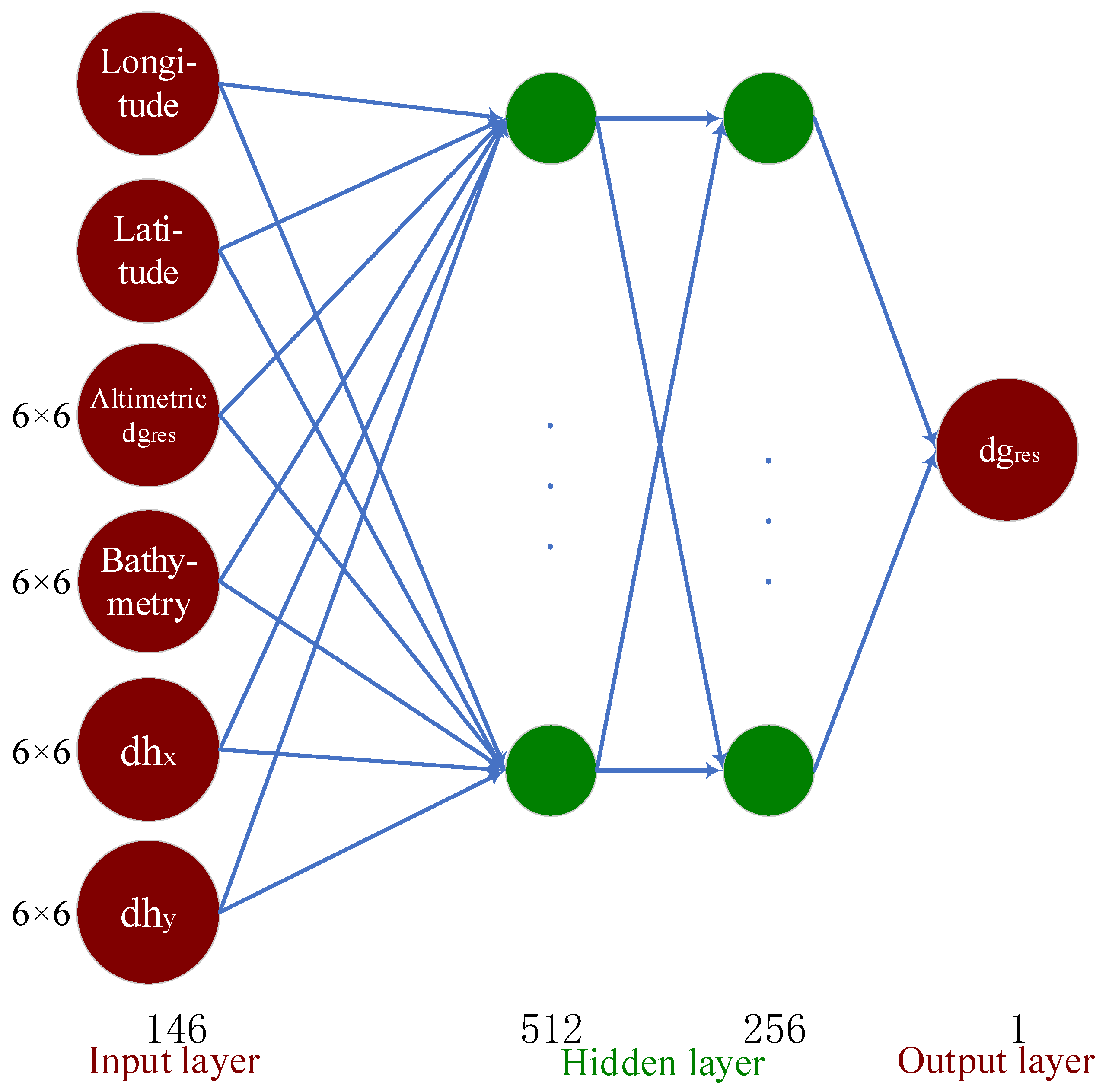
2.2.1. Structure of MLP

As various features in data can be recognized by neural networks from a small data set, a neural network can be applied in this study to improve the accuracy of altimeter-derived gravity by using sparsely and unevenly distributed shipborne data. MLP neural network is a typical feedforward artificial neural network, mapping a set of inputs to a set of desired outputs [39]. As this study is essentially a regression problem of mapping several input variables to an output variable, MLP is used in this research.
MLP, whose structure is shown in Figure 3, is composed of one input layer, one or more hidden layers and one output layer [39,40,41]. The input layer is the holding site for inputs, including several source nodes whose number is as same as that of input variables. The output layer and hidden layers are composed of output variables and neurons, respectively. Nodes in adjacent layers are connected, but nodes in the same layer are not connected. In this research, we select two hidden layers with 512 neurons in the first layer and 256 neurons in the second layer.
The output y of a neuron in hidden layers is calculated by [39]
y = f ( W x + b )
where x is the input vector of the neuron. W and b represent the connection weight vector and the bias vector, respectively. f ( ) is the activation function for nonlinear calculation, and is tanh in the regression problem. As this is a regression problem and outputs are arbitrary, activation functions should not be used in the last layer [42]. Outputs in the output layer can be obtained by
y = W x + b
While precision of altimeter-derived gravity anomalies is affected by water depth as listed in Table 3, water depth has little effect on precision of shipborne gravity. The accuracy of shipborne data since 1990 is 3.93 mGal, evaluated by crossover gravity discrepancies. The STD of altimeter-derived gravity anomalies ( m A ) can be calculated from the STD of differences ( m A S ) between altimeter-derived and shipborne data by
m A = m A S 2 m s 2
where m S is the STD of shipborne data. The differences between altimeter-derived and shipborne gravity anomalies are listed in Table 3. As the accuracy of shipborne data since 1990 in shallow waters is 3.93 mGal, the accuracy of altimeter-derived gravity anomalies is worse than that of shipborne data since 1990 when water depth is less than 50 m.
Large submarine topography slopes have effects on accuracy of altimeter-derived and shipborne gravity. As listed in Table 2 and Table 4, the STD of altimeter-derived gravity is greater than that of shipborne data when at least one of meridian and main vertical components of the slope is greater than 100 m/arcmin. Therefore, the refined area is defined as the area where the submarine topography slope is larger than 100 m/arcmin or the bathymetry is smaller than 50 m. Shipborne gravity since 1990 can be used to correct altimeter-derived gravity in the refined area.
Based on remove-restore method, residual gravity anomaly d g r e s at a point is obtained by
d g r e s = d g d g r e f
where d g represents the gravity anomaly, and d g r e f is the gravity anomaly calculated from EGM2008 (the reference gravity model).
Marine gravity anomalies depend on submarine topographic undulation and crustal density variations. There is no exact density model, so bathymetry is only considered in this paper. The submarine topography slope is the first derivative of submarine topography with respect to distance, so slopes mainly include high-frequency signals of submarine topography. Meanwhile, submarine topography slopes in an area also contain submarine topography signals outside the area. Therefore, the input and output variables are selected as shown in Figure 3. Input variables include the longitude and latitude of the observation point. Input variables also include altimeter-derived residual gravity anomalies, bathymetry and submarine topography slopes at grid points in area of 6’ × 6’ around observation points (in Figure 4). The submarine topography and its slopes are obtained from ETOPO1. While observation points for training are shipborne points since 1990 in the refined area, those for predicting are grid points in the refined area. The output variable is the refined gravity anomaly at the observation point.

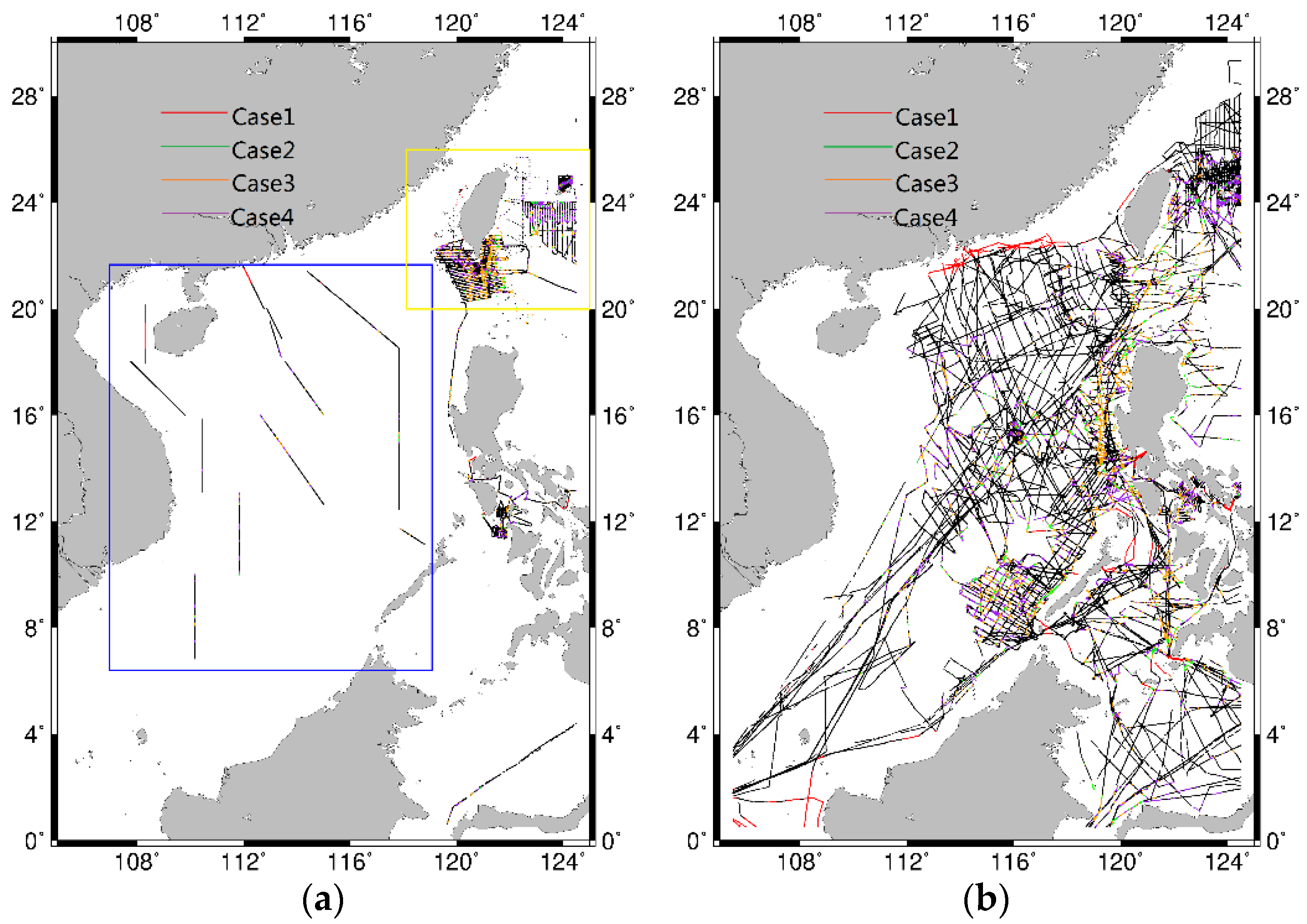
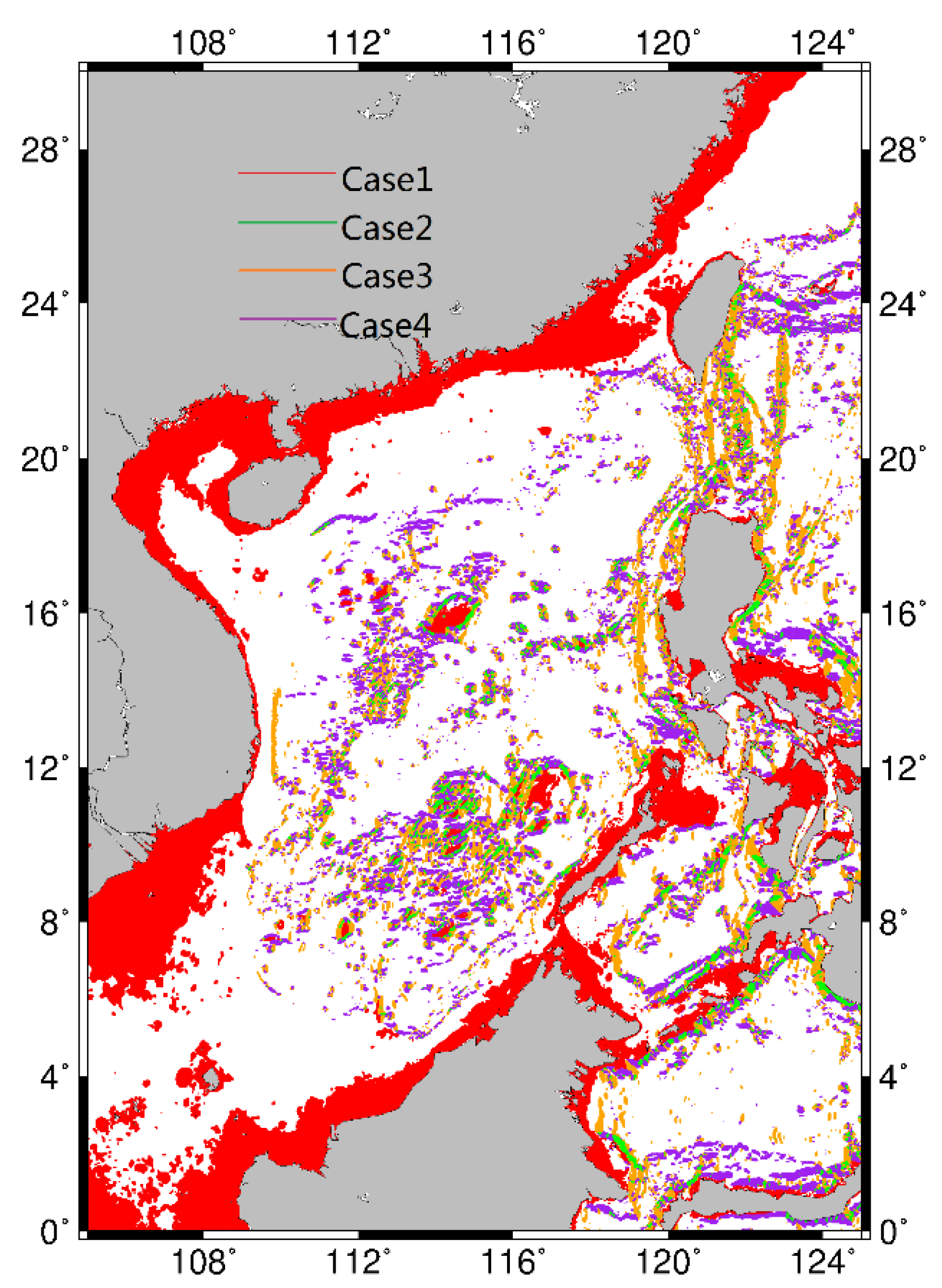
2.2.2. Refined Area Classification

The refined area refers to the area where the submarine topography slope is larger than 100 m/arcmin or the bathymetry is smaller than 50 m. While shipborne gravity anomalies used as the desired value of outputs for training the MLP are measured since 1990 in the refined area, ship-borne data measured before 1990 in the refined area are selected as the testing shipborne data. STD of differences between shipborne gravity anomalies since 1990 and SCSGA V1.0 is about 5.5 mGal. The shipborne data since 1990, which differs less than 5.5 mGal from SCSGA V1.0, are used as training shipborne data to train MLP model. Shipborne data shown in Figure 1 for training and for testing are independent of each other.
We can classify data in the refined area into seven categories, as listed in Table 5. In the SCS, the sea area with a submarine topography slope greater than 100 m/arcmin and water depth less than 50 m is very small. The SCS is divided into a 1’ × 1’ grid. There are about 1.4 million grid points in the ocean. The number of grid points is only 1623 (about 0.1% of the total number) in areas where the submarine topography slope is larger than 100 m/arcmin and the bathymetry is smaller than 50 m. Thus, data in the areas where the bathymetry is smaller than 50 m are defined as data in Case1.

2.2.3. Training and Predicting

As the structure of MLP neural network, input variables and output variables are determined, we can train the MLP model by following steps.
First, input variables should be standardized to reduce the difference between values of input variables. As a result that the shipborne data for training are not evenly distributed in this study, values of input variables for training and predicting are standardized together by removing the mean and scaling to unit variance.
Second, MLP neural network should be initialized, including randomly generating initial values of connection weight vectors and bias vectors. The structure of MLP neural network with batch size of 256 is constructed, as listed in Table 6. Loss function is mean square error to evaluate the consistence between target values and desired values of outputs. L2 regularization term with alpha of 0.01 is applied for preventing overfitting. Moreover, weights are updated by using optimization algorithm of Adam [43] with the learning rate of 10−4. Taking overfitting of training and observation errors of shipborne gravity into account, the iteration threshold and maximum number of iterations should be determined through testing, so that the determination coefficient R2 for training is approximately 0.7. Therefore, the MLP models are established by the MLP training.
Finally, corrected residual gravity anomalies at grid points can be predicted by the MLP model from input variables. By restoring gravity anomalies of EGM2008, the new gravity anomaly model at 1’ × 1’ grids can be determined.

3. Results

3.1. Refining the Gravity Model by Classification

Input variables of MLP contain altimeter-derived residual gravity anomalies, bathymetry and submarine topography slopes at grid points in area of 6’ × 6’ around observation points. The position information of observation points is also part of input variable, as shown in Figure 3. Output variables of MLP are refined gravity anomalies at observation points. Training data in different cases listed in Table 5 can be used to establish the corresponding MLP model, respectively.
First, the structure of MPL neural network is constructed as described in Section 2.2.1. The input variables include the position of the observation point and geophysical values at grid points in area of 6’ × 6’ around the observation point. The refined residual gravity anomalies at observation points are outputs. Second, using the training shipborne data since 1990 in Cases1 to 4 as the outputs of MLP, four MLP models are established, respectively. Then the four MLP models are respectively used to predict residual gravity anomalies at grid points (in Figure 5) in Cases1 to 4. Finally, refined gravity anomalies at grid points in the refined area are obtained from refined residual gravity anomalies by restoring gravity anomalies of EGM2008. Moreover, gravity anomalies at grid points not in the refined area are corresponding values of SCSGA V1.0. Therefore, the refined gravity anomaly model named SCSGA V1.1 is established.
Shipborne data measured before 1990 in the refined area are selected as testing shipborne data. The testing shipborne data are used to validate the new gravity anomaly model, as listed in Table 7. Compared with the testing shipborne data, RMS of differences (difference RMS) for SCSGA V1.0 is 0.14 mGal larger than that for SCSGA V1.1. Moreover, the mean of differences between SGSGA V1.1 and the testing shipborne data is closer to 0 mGal than that when replacing SGSGA V1.1 with SGSGA V1.0. The result suggests that SCSGA V1.1 determined by MLP neural network has the higher precision in shallow waters and areas with large submarine topography slopes, compared with SCSGA V1.0.
The difference RMS between SGSGA V1.1 and the testing shipborne data is respectively compared with that when replacing SGSGA V1.1 with SGSGA V1.0 in Cases1 to 4. The difference RMS decreases by 2.5% in Case1, 1.9% in Case2, 3.5% in Case3 and 1.6% in Case4. The precision of SGSGA V1.1 is higher than that of SGSGA V1.0 in every case. These results suggest that refining altimeter-derived gravity in the refined area from shipborne gravity by MLP is reliable.

3.2. Refining the Gravity Model as a Whole

As submarine topography and its slopes are part of input variables, the mapping from submarine topography and its slopes to outputs is taken into account in training MLP neural network. Therefore, it can be inferred that we can obtain a good gravity anomaly model without classification. All of training shipborne data are used to train an MLP model. Then, the refined gravity anomaly model on a 1′ × 1′ grid (SCSGA V1.2) is determined by the MLP model.
Gravity anomalies at grid points in the refined area are corrected, so SGSCS V1.2 is compared with the testing shipborne data, as listed in Table 8. The difference RMS for SGSCS V1.2 is 2.4% smaller than that for SGSCS V1.0, and the difference mean for the former is closer to 0 mGal than that for the latter.
Compared with the testing shipborne data in Cases1 to 4, the difference RMS for SGSCS V1.2 is 1.9%, 2.4%, 3.1% and 2.5% smaller than that for SGSCS V1.0, respectively. The accuracy improvement in Case1 is the smallest due to the little number of training data in the area. Similarly, the accuracy improvement in Case3 is the largest because of the large number of training data in the area.
Validated by the testing shipborne data, SGSCS V1.2 has higher accuracy than SGSCS V1.1 in Case2 and Case4, while the accuracy is opposite in Case1 and Case3. The conclusion can be drawn that gravity anomaly models refined by one MLP model in all cases and different MLP models in different cases have similar accuracy, which verifies the inference we make at the beginning of Section 3.2. Therefore, for refining gravity models based on neural networks, only one MLP model need to be established in the refined area, and the region does not need to be classified according to input variables.

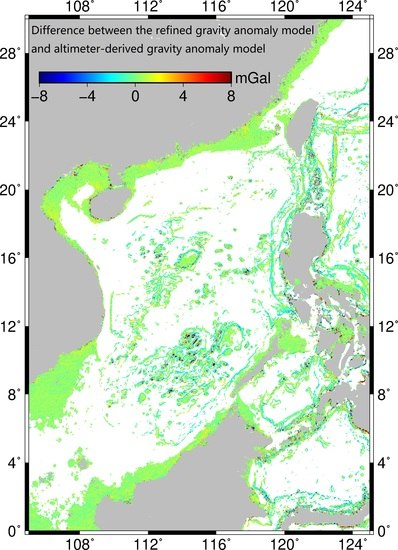
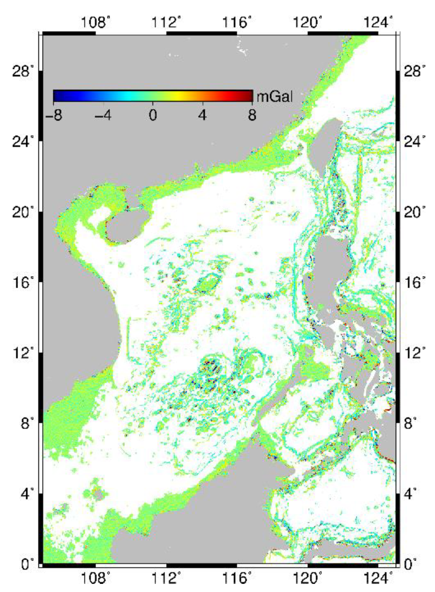
3.3. Analysis of the Refined Gravity Anomaly Model

Considering that the distribution of training data may affect the accuracy of refined gravity models, the research region is divided into two regions including Taiwan sea area (Region A, covering 20° N~26° N and 118° E~125° E) and SCS area except Taiwan area (Region B), as shown in Figure 1. The testing shipborne data are compared with SGSCS V1.2 in different regions, as listed in Table 9. Validated by the testing shipborne data, the accuracy of SGSCS V1.2 is 4.4% and 2.2% higher than that of SGSCS V1.0 in Region A and Region B, respectively.
In Region A, difference RMS between SGSCS V1.2 and the testing shipborne data is 2.1%, 5.3%, 3.4% and 4.9% smaller than that when replacing SGSGA V1.2 with SGSGA V1.0 in Cases1 to 4, respectively. In Region B, compared with the testing shipborne data, difference RMS for SGSCS V1.2 is 1.9%, 2.1%, 2.5% and 2.2% smaller than that SGSCS V1.0 in Cases1 to 4, respectively. Compared with SCSGA V1.0, the accuracy improvement of SCSGA V1.2 in Region A is greater than that in Region B, which can be attributed to the denser distribution of the training shipborne data in Region A than in Region B as shown in Figure 1. We can draw the conclusions that the accuracy improvement of refined gravity models compared with altimeter-derived gravity models is related to the distribution of training data. The accuracy improvement is more obviously in the region with a large amount of training data than that in the region with few training data. Moreover, in the region with few training data, the accuracy of refined gravity is also improved based on MLP neural network compared with that of altimeter-derived gravity.
Whether the choice of input variables (bathymetry and submarine topography slopes) of MLP neural network is appropriate needs to be discussed. First, bathymetry and submarine topography slopes are removed from input variables of MLP, which are used to refine altimeter-derived gravity anomalies to obtain the gravity anomaly model M1. Second, only submarine topography slopes are removed from input variables of MLP, which are used to establish the refined gravity anomaly model M2. Finally, the refined gravity anomaly model M3 is determined by MLP whose input variables do not include bathymetry.
The testing shipborne data are used to evaluate the accuracy of M1, M2 and M3, as listed in Table 10. The accuracy of M1, M2 and M3 is higher than that of SCSGA V1.0. The result suggests that MLP neural network method is viable to refine altimeter-derived gravity from shipborne data. However, the accuracy of M1, M2 and M3 is lower than that of SCSGA V1.2, which is due to less input variables. M1 have the lowest precision, which can be attributed to the fact that the MLP neural network used to obtain M1 have the least input variables. These results suggest that bathymetry and submarine topography slopes play important roles in refining altimeter-derived gravity anomalies.
In Case1, where water depth is shallower than 50 m and most of topography slopes are small, the accuracy of M3 is lower than that of other models. This result shows that submarine topography slopes cannot be used to refine altimeter-derived gravity in shallow waters alone without bathymetry. In Cases2 to 4, the accuracy of M3 is higher than that of M1 and M2, suggesting that submarine topography slopes play a more important role than bathymetry in refining altimeter-derived gravity in areas where submarine topography slopes are large.
These results shows that the choice of input variables (bathymetry and submarine topography slopes) of MLP neural network is appropriate.
Finally, SCSGA V1.2 and SCSGA V1.0 are compared, as shown in Figure 6. The largest corrections locate in coastal areas and areas with many islands and reefs, which can be attributed to the fact that land and reefs contaminate altimeter waveforms. The differences are analyzed respectively in shallow waters with different bathymetry, as listed in Table 11. The differences increase with the decrease of water depth, which can be due to the reason that the accuracy of altimeter-derived gravity decreases as the water depth decreases as listed in Table 3. Then differences between SCSGA V1.2 and SCSGA V1.0 are analyzed in areas with different submarine topography slopes, as listed in Table 11. The differences increase as submarine topography slopes increase, whose reason is that submarine topography slopes have effects on the accuracy of altimeter-derived and shipborne gravity as listed in Table 1 and Table 4. In general, the results are consistent with effects of water depth and submarine topography slopes on altimeter-derived gravity. Therefore, the results further verify the reliability of refining altimeter-derived gravity from shipborne data by using MLP.

4. Discussion

In order to analyze the correction of altimeter-derived gravity models in frequency domain by shipborne data, SCSGA V1.0 and SCSGA V1.2 are respectively compared with shipborne data. As shipborne gravity provided by NCEI contains large noises that will affect analysis in the frequency domain, a section of the shipborne gravity measured in 2005 provided by MNR with higher accuracy is selected, as shown in Figure 7. The sample interval of the shipborne data is about 0.34 km, and there are no two consecutive missing data in the data. Moreover, the shipborne data are located at the edge of the central basin of the SCS, where slopes of submarine topography are large. According to ETOPO1 model in the area, the deepest depth is about 4400 m, and the shallowest depth is about 1700 m. As submarine topography slopes are greater than 100 m/arcmin along the shipborne track, the gravity anomalies at the shipborne observation points interpolated by SCSGA V1.0 and SCSGA V1.2 are different.
The shipborne data are interpolated into an equally spaced sequence with an interval of 0.34 km, and differences between the sequence and gravity anomaly models are calculated. The differences are analyzed by power spectral density (PSD) [44,45], as shown in Figure 8. The PSD of differences between shipborne data and SCSGA V1.0 is similar to that between shipborne data and SCSGA V1.2 for wavelengths longer than 10 km. For wavelengths shorter than 2.5 km, PSD of differences between SCSGA V1.0 and shipborne data is divided by that between SCSGA V1.2 and shipborne data to obtain the PSD ration, as shown in Figure 8. Most values of the PSD ratio are greater than 1. Therefore, the PSD of differences between shipborne data and SCSGA V1.0 is larger than that when replacing V1.0 with V1.2 for wavelengths shorter than 2.5 km, suggesting that the shipborne data mainly improve the high frequency signal of the gravity model. The result can be attributed to the following. Ground track interval at equator of altimetry satellites used to derive SCSGA V1.0 is about 2.5 km [37,46], so gravity signals for wavelength shorter than 2.5 km are weak in SCSGA V1.0. Moreover, the resolution of shipborne gravity with small sampling interval is greater than 1 km. Therefore, shipborne data can be used to improve high frequency signals of altimeter-derived gravity models by MLP neural network.

5. Conclusions

Altimeter-derived gravity models are refined by shipborne data based on an MLP neural network in this paper. As gravity anomalies are related with spatial positions, input variables include the longitude and latitude of observation points. As gravity anomalies are also related with submarine topography and its slopes, input variables include altimeter-derived residual gravity anomalies (from SCSGA 1.0), bathymetry (from ETOPO1) and submarine topography slopes (from ETOPO1) at grid points in an area of 6’ × 6’ around the observation point. The refined residual gravity anomalies at observation points are output variables. For training the MLP model, shipborne observation points since 1990 in the refined area (where the submarine topography slope is larger than 100 m/arcmin or the bathymetry is smaller than 50 m) are the observation points of MLP neural network, and shipborne gravity anomalies at observation points are desired outputs. Grid points in the refined area are the observation points of MLP neural network, when using MLP model to predict refined gravity anomaly models.
Data are classified according to submarine topography and its slopes of the area where they are located. Training data in each case are respectively used to train the corresponding MLP model. Refined residual gravity anomalies in each case are predicted by the corresponding MLP model to establish the refined gravity anomaly model SCSGA V1.1. Meanwhile, one MLP model is constructed from all of training data in the refined area, and used to predict refined residual gravity anomalies at grid points in the refined area to establish the model SCSGA V1.2.
Shipborne gravity anomalies before 1990 in the refined area are taken as the testing shipborne data to evaluate the precision of gravity anomaly models. Validated by the testing shipborne data, the accuracy of SCSGA V1.2 is 0.14 mGal higher than that of SCSGA V1.0 in the SCS. Compared with SCSGA V1.0, the accuracy of SCSGA V1.2 in Case1, Case2, Case4 and Case3 is improved, as the number of training data increases sequentially. Compared with the testing shipborne data, the RMS difference for SCSGA V1.2 is 0.26 mGal (4.4%) smaller than that for SCSGA V1.0 in Taiwan sea area where the distribution of training data is dense. Meanwhile, in the SCS, except the Taiwan area, the accuracy improvement of SCSGA V1.2 is about 2.2% compared with SCSGA V1.0. The accuracy of SCSGA V1.1 is similar to that of SCSGA V1.2. Finally, PSD is used to analyze differences between gravity anomaly models and shipborne data, which suggests that shipborne data mainly improve signals of gravity models for wavelengths shorter than 2.5 km.
When using MLP neural network to correct altimeter-derived gravity model by shipborne data, both of the spatial position and submarine topography should be considered. Therefore, the MLP neural network overcomes the problem that the traditional method can only be used to correct gravity models in a limited radius around shipborne observation points. Compared with the altimeter-derived gravity model, the refined gravity model not only has a great accuracy improvement in areas where training data are concentrated, but also has an accuracy improvement in other areas.

Author Contributions

Conceptualization, J.G. (Jinyun Guo); data curation, C.Z.; formal analysis, C.Z., J.Y. and X.J.; funding acquisition, J.G. (Jinyun Guo); investigation, C.Z., X.J. and C.L.; methodology, C.Z., J.G. (Jinyun Guo), X.J. and J.G. (Jinyao Gao); project administration, J.G. (Jinyun Guo); resources, J.G. (Jinyun Guo) and J.G. (Jinyao Gao); software, C.Z. and J.Y.; supervision, J.G. (Jinyun Guo); validation, C.Z. and C.L.; visualization, C.Z.; writing—original draft, C.Z.; writing—review and editing, J.G. (Jinyun Guo). All authors have read and agreed to the published version of the manuscript.

Funding

This research was funded by the National Natural Science Foundation of China (Grant Nos. 41774001, 41374009), the SDUST Research Fund (Grant No. 2014TDJH101) and the Autonomous and Controllable Special Project for Surveying and Mapping of China (Grant No. 816-517).

Institutional Review Board Statement

Not applicable.

Informed Consent Statement

Not applicable.

Data Availability Statement

Publicly available datasets were used in this study. The altimeter products were produced and distributed by Aviso+ (https://www.aviso.altimetry.fr/), as part of the Ssalto ground processing segment. The NCEI shipborne data can be found here: https://maps.ngdc.noaa.gov/viewers/geophysics/. ETOPO1 can be found here: http://www.ngdc.noaa.gov/mgg/global/global.html. EGM2008 can be found here: http://earth-info.nga.mil/GandG/wgs84/gravitymod/egm2008.

Acknowledgments

We are very grateful to AVISO and National Satellite Ocean Application Service of China for providing altimetric data, and NCEI and Second Institute of Oceanography of MNR, China, for providing ship-borne gravimetric data.

Conflicts of Interest

The authors declare no conflict of interest.

References

  1. King-Hele, D. The shape of the Earth. Science 1976, 192, 1293–1300. [Google Scholar] [CrossRef] [PubMed]
  2. Rathnayake, S.; Tenzer, R. Interpretation of the lithospheric structure beneath the Indian Ocean from gravity gradient data. J. Asian Earth Sci. 2019, 183, 103934. [Google Scholar] [CrossRef]
  3. Tenzer, R.; Gladkikh, V.; Novak, P.; Vajda, P. Spatial and spectral analysis of refined gravity data for modelling the crust-mantle interface and mantle-lithosphere structure. Surv. Geophys. 2012, 33, 817–839. [Google Scholar] [CrossRef]
  4. Hotta, H.; Kubota, R.; Ishikawa, H.; Oshida, A.; Okada, C.; Matsuda, T.; Asakawa, E. The goal of the integrated ocean resources survey system (“INORSS”). In Next-generation Technology for Ocean Resources Exploration of “SIP”; OCEANS—MTS/IEEE Kobe Techno-Oceans Conference: Kobe, Japan; New York, NY, USA, 2018. [Google Scholar]
  5. Bobojc, A. Application of gravity gradients in the process of GOCE orbit determination. Acta Geophys. 2016, 64, 521–540. [Google Scholar] [CrossRef] [Green Version]
  6. Sun, X.; Chen, P.; Macabiau, C.; Han, C. Low-Earth orbit determination from gravity gradient measurements. Acta Astronaut. 2016, 123, 350–362. [Google Scholar] [CrossRef] [Green Version]
  7. Andersen, O.B.; Knudsen, P. The DTU17 global marine gravity field: First validation results. In Fiducial Reference Measurements for Altimetry, International Association of Geodesy Symposia; Mertikas, S., Pail, R., Eds.; Springer: Berlin/Heidelberg, Germany, 2019; Volume 150. [Google Scholar]
  8. Sandwell, D.T.; Harper, H.; Tozer, B.; Smith, W.H.F. Gravity field recovery from geodetic altimeter missions. Adv. Space Res. 2019. [Google Scholar] [CrossRef]
  9. Sandwell, D.T.; Muller, R.D.; Smith, W.H.F.; Garcia, E.; Francis, R. New global marine gravity model from CryoSat-2 and Jason-1 reveals buried tectonic structure. Science 2014, 346, 65–67. [Google Scholar] [CrossRef] [PubMed]
  10. Hwang, C.; Hsu, H.Y. Shallow-water gravity anomalies from satellite altimetry: Case studies in the east China sea and Taiwan strait. J. Chin. Inst. Eng. 2008, 31, 841–851. [Google Scholar] [CrossRef]
  11. Zhang, S.; Sandwell, D.T.; Jin, T.; Li, D. Inversion of marine gravity anomalies over southeastern China seas from multi-satellite altimeter vertical deflections. J. Appl. Geophys. 2017, 137, 128–137. [Google Scholar] [CrossRef] [Green Version]
  12. Sandwell, D.T.; Gille, S.T.; Orcutt, J.; Smith, W.H.F. Bathymetry from space is now possible. EOS Trans. Am. Geophys. Un. 2003, 84, 37–44. [Google Scholar] [CrossRef]
  13. Kim, J.W.; von Frese, R.R.B.; Lee, B.Y.; Roman, D.R.; Doh, S.-J. Altimetry-derived gravity predictions of bathymetry by the gravity-geologic method. Pure Appl. Geophys. 2010, 168, 815–826. [Google Scholar] [CrossRef]
  14. Fan, D.; Li, S.; Li, X.; Yang, J.; Wan, X. Seafloor Topography estimation from gravity anomaly and vertical gravity gradient using nonlinear iterative least square method. Remote Sens. 2021, 13, 64. [Google Scholar] [CrossRef]
  15. Zaki, A.; Mansi, A.H.; Selim, M.; Rabah, M.; El-Fiky, G. Comparison of satellite altimetric gravity and global geopotential models with shipborne gravity in the Red Sea. Mar. Geodesy 2018, 41, 258–269. [Google Scholar] [CrossRef]
  16. Zhu, C.; Guo, J.; Hwang, C.; Gao, J.; Yuan, J.; Liu, X. How HY-2A/GM altimeter performs in marine gravity derivation: Assessment in the South China Sea. Geophys. J. Int. 2019, 219, 1056–1064. [Google Scholar] [CrossRef]
  17. Li, Z.; Liu, X.; Guo, J.; Zhu, C.; Yuan, J.; Gao, J.; Gao, Y.; Ji, B. Performance of Jason-2/GM altimeter in deriving marine gravity with the waveform derivative retracking method: A case study in the South China Sea. Arab. J. Geosci. 2020, 13, 939. [Google Scholar] [CrossRef]
  18. Huang, M.; Wang, R.; Zhai, G.; Ouyang, Y. Integrated data processing for multi-satellite missions and recovery of marine gravity field. Geomat. Informat. Sci. Wuhan Univ. 2007, 32, 988–993. [Google Scholar] [CrossRef] [Green Version]
  19. Wu, Y.H. Regional Gravity Field Modeling from Heterogeneous Data Sets by Using Poisson Wavelets Radial Basis Functions. Ph.D. Thesis, Wuhan University, Wuhan, China, 2016. [Google Scholar]
  20. Guo, J.; Liu, X.; Chen, Y.; Wang, J.; Li, C. Local normal height connection across sea with ship-borne gravimetry and GNSS techniques. Mar. Geophys. Res. 2014, 35, 141–148. [Google Scholar] [CrossRef]
  21. Hwang, C.; Parsons, B. Gravity anomalies derived from Seasat, Geosat, ERS-1 and TOPEX/POSEIDON altimetry and ship gravity: A case study over the Reykjanes Ridge. Geophys. J. Int. 1995, 122, 551–568. [Google Scholar] [CrossRef]
  22. Paolo, F.S.; Molina, E.C. Integrated marine gravity field in the Brazilian coast from altimeter-derived sea surface gradient and shipborne gravity. J. Geodynam. 2010, 50, 347–354. [Google Scholar] [CrossRef]
  23. Wu, Y.H.; Luo, Z.C.; Zhou, B.Y. Regional gravity modeling based on heterogeneous data sets by using Poisson wavelets radial basis functions. Chin. J. Geophys. 2016, 59, 852–864. [Google Scholar]
  24. Samuel, A.L. Some studies in machine learning using the game of checkers. IBM J. 1959, 3, 211–229. [Google Scholar] [CrossRef]
  25. Bengio, Y.; Lecun, Y. Scaling learning algorithms towards AI. In Large-Scale Kernel Machines; Chapelle, O., Decoste, D., Eds.; MIT Press: Cambridge, UK, 2007; pp. 321–358. [Google Scholar]
  26. Bengio, Y.; Delalleau, O. On the expressive power of deep architectures. In Proceeding of the 14th International Conference on Discovery Science, Espoo, Finland, 5–7 October 2011; Springer: Berlin/Heidelberg, Germany, 2011; pp. 18–36. [Google Scholar]
  27. Widiasari, I.R.; Nugroho, L.E.; Widyawan, W. Deep learning multilayer perceptron (MLP) for flood prediction model using wireless sensor network based hydrology time series data mining. In Proceedings of the International Conference on Innovative and Creative Information Technology, Salatiga, Indonesia, 2–4 November 2017; IEEE: New York, NY, USA, 2017. [Google Scholar]
  28. Vafaeipour, M.; Rahbari, O.; Rosen, M.A.; Fazelpour, F.; Ansarirad, P. Application of sliding window technique for prediction of wind velocity time series. Int. J. Energy Environ. Eng. 2014, 5, 105. [Google Scholar] [CrossRef] [Green Version]
  29. Voyant, C.; Nivet, M.L.; Paoli, C.; Muselli, M.; Notton, G. Meteorological time series forecasting based on MLP modelling using heterogeneous transfer functions. J. Phys. Conf. Ser. 2015, 574, 012064. [Google Scholar] [CrossRef] [Green Version]
  30. Voyant, C.; Paoli, C.; Muselli, M.; Nivet, M.L. Multi-horizon solar radiation forecasting for Mediterranean locations using time series models. Renew. Sustain. Energy Rev. 2013, 28, 44–52. [Google Scholar] [CrossRef] [Green Version]
  31. Guan, D.L.; Ke, X.P.; Wang, Y. Basement structures of East and South China Seas and adjacent regions from gravity inversion. J. Asian Earth Sci. 2016, 117, 242–255. [Google Scholar] [CrossRef]
  32. Hwang, C.; Chang, E.T.Y. Seafloor secrets revealed. Science 2014, 346, 32–33. [Google Scholar] [CrossRef] [PubMed]
  33. Pavlis, N.K.; Holmes, S.A.; Kenyon, S.C.; Factor, J.K. The development and evaluation of the Earth Gravitational Model 2008 (EGM2008). J. Geophys. Res. 2012, 117, B04406. [Google Scholar] [CrossRef] [Green Version]
  34. Sandwell, D.T.; Garcia, E.; Soofi, K.; Wessel, P.; Chandler, M.; Smith, W.H.F. Toward 1-mGal accuracy in global marine gravity from CryoSat-2, Envisat, and Jason-1. Lead. Edge 2013, 32, 892–899. [Google Scholar] [CrossRef] [Green Version]
  35. Amante, C.; Eakins, B.W. ETOPO1 1 arc-minute global relief model: Procedures, data sources and analysis. In NOAA Technical Memorandum NESDIS NGDC-24; National Geophysical Data Center, NOAA: Miami, FL, USA, 2009. [Google Scholar]
  36. Wessel, P.; Watts, A.B. On the accuracy of marine gravity measurements. J. Geophys. Res. Solid Earth 1988, 93, 393–413. [Google Scholar] [CrossRef]
  37. Zhu, C.; Guo, J.; Gao, J.; Liu, X.; Hwang, C.; Yu, S.; Yuan, J.; Ji, B.; Guan, B. Marine gravity determined from multi-satellite GM/ERM altimeter data over the South China Sea: SCSGA V1.0. J. Geodesy 2020, 94, 50. [Google Scholar] [CrossRef]
  38. Hwang, C. Inverse Vening Meinesz formula and deflection-geoid formula: Applications to the predictions of gravity and geoid over the South China Sea. J. Geodesy 1998, 72, 304–312. [Google Scholar] [CrossRef]
  39. Shiblee, M.; Kalra, P.K.; Chandra, B. Time series prediction with multilayer perceptron (MLP): A new generalized error based approach. In International Conference on Neural Information Processing, Auckland, New Zealand, 2008; Koppen, M., Ed.; Springer: Berlin/Heidelberg, Germany, 2008; pp. 37–44. [Google Scholar]
  40. Bishop, C.M. Neural Networks for Pattern Recognition; Oxford University Press: Oxford, UK, 1995. [Google Scholar]
  41. Cagli, E.; Dumas, C.; Prouff, E. Convolutional Neural Networks with Data Augmentation Against Jitter-Based Countermeasures. In International Conference on Cryptographic Hardware and Embedded Systems, Taiwan, China, 2017; Fischer, W., Homma, N., Eds.; Springer: Berlin/Heidelberg, Germany, 2017; pp. 45–68. [Google Scholar]
  42. Chollet, F. Deep Learning with Python; Manning Publication Co.: New York, NY, USA, 2018. [Google Scholar]
  43. Kingma, D.P.; Ba, J. Adam: A method for stochastic optimization. In Proccedings of the International Conference on Learning Representations, San Diego, CA, USA, 7–9 May 2015. [Google Scholar]
  44. Pujol, M.-I.; Schaeffer, P.; Faugère, Y.; Raynal, M.; Dibarboure, G.; Picot, N. Gauging the improvement of recent mean sea surface models: A new approach for identifying and quantifying their errors. J. Geophys. Res. Ocean 2018, 123, 5889–5911. [Google Scholar] [CrossRef]
  45. Yuan, J.; Guo, J.; Niu, Y.; Zhu, C.; Li, Z. Mean sea surface model over the sea of Japan determined from multi-satellite altimeter data and tide gauge records. Remote Sens. 2020, 12, 4168. [Google Scholar] [CrossRef]
  46. CNES. Along-Track Level-2+ (L2P) SLA Product Handbook; SALP-MU-P-EA-23150-CLS, Issue1.0; CNES: Paris, France, 2017.
Figure 1. Shipborne gravity data tracks. (a) Shipborne data measured since 1990, (b) shipborne data measured before 1990. The tracks in the blue box are from Ministry of Natural Resources of P. R. China (MNR). The data in black are not in the refined area. The region in the yellow box is region A.
Remotesensing 13 00607 g001
Figure 2. Tracks of altimetric data used to determine altimetric gravity anomaly model around the South China Sea (SCSGA) V1.0.
Remotesensing 13 00607 g002
Figure 3. Structure of multi-layer perceptron (MLP): dhx and dhy are respectively prime vertical and meridian components of submarine topography slopes and dgres represents residual gravity anomalies.
Remotesensing 13 00607 g003
Figure 4. Observation points and surrounding grid points.
Remotesensing 13 00607 g004
Figure 5. Distribution of grid points in different cases.
Remotesensing 13 00607 g005
Figure 6. Differences between SCSGA V1.2 and SCSGA V1.0.
Remotesensing 13 00607 g006
Figure 7. Shipborne gravity track and surrounding submarine topography for power spectral density (PSD) analysis.
Remotesensing 13 00607 g007
Figure 8. PSD of differences between shipborne data and gravity models.
Remotesensing 13 00607 g008
Table 1. Accuracy of shipborne data in different areas.
Submarine Topography Slope
(m/arcmin a)
Shipborne Data before 1990
(mGal)
Shipborne Data Since 1990
(mGal)
All4.413.93
N > 50 or E > 50 b4.554.16
N > 100 or E > 1004.894.17
N > 150 or E > 1505.104.38
a 1 m/arcmin is equal to 0.54 m/km. b N: meridian component E: prime vertical component.
Table 2. Information on altimetric data of geodetic missions (GMs).
SatellitePeriodInter-Track Distance at Equator (km)Sampling Interval along Track (km)
ERS-194.04–95.0376.6
Jason-112.05–13.0675.8
Jason-217.07–19.0275.8
HY-2A16.03–18.07156.5
SARAL–AltiKa16.07–18.1056.9
CryoSat-211.01–18.072.56.4
Table 3. Differences between SCSGA V1.0 and shipborne data since 1990 in shallow waters.
Bathymetry (m)0–1010–2020–3030–4040–5050–6060–7070–100
RMS (mGal)10.487.806.547.636.415.594.483.89
STD (mGal)9.807.746.317.596.365.534.483.84
Table 4. Differences between SCSGA V1.0 and shipborne data since 1990 in deep waters with different submarine topography slopes.
Slopes (m/arcmin)AllE > 50 or N > 50E > 100 or N > 100E > 150 or N > 150
RMS (mGal)5.365.886.286.37
STD (mGal)5.355.856.226.30
Table 5. Classification.
CategoryBathymetry
50 m
Submarine Topography SlopeNumber of SamplesNumber of Predicted Grid Points
Prime Vertical
100 m/arcmin
Meridian
100 m/arcmin
Case1< 795245,314
< >
< >
< > >
Case2> > 343152,692
Case3> 761274,093
Case4> 526076,225
Table 6. Structure of MLP neural network.
LayerVariableVector Size
Input layerInput (256,146)
Output(256,146)
Hidden layer1Input (256,146)
Output(256,512)
2Input (256,512)
Output(256,256)
Output layerInput (256,256)
Output(256,1)
Table 7. Statistics of differences between gravity models and the testing shipborne data (in mGal).
Refined AreaCase1Case2Case3Case4
Number99,04811,34324,22230,81532,668
V1.0-
NCEI
MEAN−0.59−0.06−0.77−0.80−0.44
STD5.785.806.165.705.54
RMS5.815.806.215.755.55
V1.1-
NCEI
MEAN−0.360.04−0.58−0.30−0.40
STD5.665.656.065.545.45
RMS5.675.656.095.555.46
Table 8. Differences between refined gravity model and the testing shipborne data (in mGal).
Refined AreaCase1Case2Case3Case4
Number99,04811,34324,22230,81532,668
V1.2-
NCEI
MEAN−0.40−0.38−0.55−0.40−0.30
STD5.655.686.045.585.40
RMS5.675.696.065.575.41
Table 9. Differences between SCSGAV1.2 and the testing shipborne data in different regions (in mGal).
Refined AreaCase1Case2Case3Case4
Region ANumber7626189168224213334
V1.0- NCEIMEAN0.14−0.850.78−0.440.28
STD5.915.756.366.155.45
RMS5.915.816.416.165.46
V1.2- NCEIMEAN0.18−1.500.70−0.220.30
STD5.655.496.035.955.18
RMS5.655.696.075.955.19
Region BNumber91,42211,15422,54028,39429,334
V1.0- NCEIMEAN−0.65−0.05−0.88−0.83−0.52
STD5.765.806.135.655.54
RMS5.805.806.195.715.56
V1.2- NCEIMEAN−0.45−0.36−0.65−0.42−0.36
STD5.655.686.035.555.43
RMS5.675.696.065.575.44
Table 10. RMS of differences between gravity models and the testing shipborne data (in mGal).
Gravity ModelRefined AreaCase1Case2Case3Case4
SCSGA V1.05.815.806.215.755.55
SCSGA V1.25.675.696.065.575.41
M15.755.776.135.665.53
M25.715.736.085.645.49
M35.705.836.055.625.46
Table 11. Differences between SCSGA V1.2 and SCSGA V1.0 in different areas (in mGal).
Depth (m)MAXMINMEANSTDRMS
0–1017.55−23.550.361.851.89
10–2015.74−15.430.401.641.69
20–3019.25−18.530.461.431.50
30–4012.67−14.420.401.251.31
40–5013.80−16.200.351.101.15
Slopes (m/arcmin)MAXMINMEANSTDRMS
N > 100 or E > 10020.05−23.78−0.182.012.02
N > 150 or E > 15019.94−23.78−0.142.232.23
N > 200 or E > 20017.52−23.78−0.112.442.44
N > 300 or E > 30017.52−21.98−0.052.862.86
Publisher’s Note: MDPI stays neutral with regard to jurisdictional claims in published maps and institutional affiliations.

