Abstract
Unmanned aerial systems (UAS) carrying commercially sold multispectral sensors equipped with a sunshine sensor, such as Parrot Sequoia, enable mapping of vegetation at high spatial resolution with a large degree of flexibility in planning data collection. It is, however, a challenge to perform radiometric correction of the images to create reflectance maps (orthomosaics with surface reflectance) and to compute vegetation indices with sufficient accuracy to enable comparisons between data collected at different times and locations. Studies have compared different radiometric correction methods applied to the Sequoia camera, but there is no consensus about a standard method that provides consistent results for all spectral bands and for different flight conditions. In this study, we perform experiments to assess the accuracy of the Parrot Sequoia camera and sunshine sensor to get an indication if the quality of the data collected is sufficient to create accurate reflectance maps. In addition, we study if there is an influence of the atmosphere on the images and suggest a workflow to collect and process images to create a reflectance map. The main findings are that the sensitivity of the camera is influenced by camera temperature and that the atmosphere influences the images. Hence, we suggest letting the camera warm up before image collection and capturing images of reflectance calibration panels at an elevation close to the maximum flying height to compensate for influence from the atmosphere. The results also show that there is a strong influence of the orientation of the sunshine sensor. This introduces noise and limits the use of the raw sunshine sensor data to compensate for differences in light conditions. To handle this noise, we fit smoothing functions to the sunshine sensor data before we perform irradiance normalization of the images. The developed workflow is evaluated against data from a handheld spectroradiometer, giving the highest correlation (R2 = 0.99) for the normalized difference vegetation index (NDVI). For the individual wavelength bands, R2 was 0.80–0.97 for the red-edge, near-infrared, and red bands.
1. Introduction
Unmanned aerial systems (UASs) are used extensively for environmental monitoring, and there has been a sharp increase in the number of studies since 2010 (e.g., [1,2]), with the largest number of publications in the field of agriculture [1]. Zarco-Tejada [3] initially demonstrated the potential to derive biophysical parameters from data collected with sensors carried by UASs, and UAS data have been used extensively for precision agriculture (e.g., [4,5]). UASs are also commonly used in forestry [1,6] and for more general environmental monitoring [2]. Major advantages of using UASs for data collection are the possibility to frequently obtain data with high spatial resolution at relatively low cost, and the flexibility to collect data with short notice and with optimal timing for the phenomena also studied under cloudy conditions (e.g., [7,8]).
The use of UASs for deriving vegetation variables related to plant health and productivity has been stimulated by commercially sold, lightweight multispectral cameras, and software such as Agisoft Metashape (Agisoft LLC, St. Petersburg, Russia) and Pix4Dmapper (Pix4D SA, Lucerne, Switzerland) simplifies the creation of three-dimensional (3D) models and orthomosaics from image data with structure-from-motion techniques [9]. The products created for vegetation monitoring are typically orthomosaics with surface reflectance or vegetation indices, such as the normalized difference vegetation index (NDVI). To enable comparisons between reflectance and vegetation indices derived from image data collected at different times, e.g., for crop growth estimates in precision agriculture or phenological studies or for comparisons between data collected with different sensors, it is crucial that the data are radiometrically consistent and that obtained surface reflectance estimates are reliable.
Surface reflectance is not directly measured by the UAS cameras. When an image is captured, the image sensor in the camera records the radiant energy (light) received by each pixel as a digital number (DN). To convert the DN to surface reflectance, a radiometric correction must be performed by (1) applying sensor related corrections to obtain the radiance received by the camera from the DN, and (2) converting the radiance received by the camera to surface reflectance [7,10,11]. Sensor-related corrections include correction for vignetting effects, which result in less light reaching the edges of the sensor [12]. They also include calibrating for different exposure settings (exposure time, aperture size), which decide the amount of light entering into the camera, and for the sensitivity of the image sensor, which influences the relationship between the radiant energy received by the sensor and the recorded DN [10]. Conversion of sensor corrected DNs to surface reflectance is applied to compensate for external factors, such as the intensity of the solar irradiance and atmospheric conditions. If images are captured in sunny conditions, there is also a need to apply corrections for varying illumination and viewing angles, as well as the anisotropic reflectance properties of the ground cover (e.g., [7,10,11]). Sensor-related corrections are sensor-specific, as described further in Section 2. Conversion of sensor corrected DNs to surface reflectance to compensate for influence of the atmosphere on the images, e.g., with atmospheric modeling or the empirical line method, and corrections for varying light conditions and viewing angles are more general methods.
A common method to convert DNs to surface reflectance in remotely sensed data is the empirical line method [13]. The method assumes that there is a linear relationship between the DNs of all pixels in an image and surface reflectance, and usually one or more reflectance calibration panels with known reflectance are used to estimate this relationship. The method has been used extensively for UAS data collected with hyperspectral cameras (e.g., [14,15,16]), red/green/blue (RGB) cameras modified to color infrared (CIR) cameras (e.g., [17,18,19]), and multispectral cameras (e.g., [20,21,22,23,24,25]). The empirical line method compensates for atmospheric effects, but UAS data usually consist of a large number of images collected during a flight in a time interval of typically 10–30 min with potentially varying light conditions. Hence, it is also important to adjust for differences in illumination conditions between images.
In order to overcome the problem with illumination variations, Honkavara et al. [26] developed a method to model relative differences in reflectance between images on the basis of a relative radiometric block adjustment following Chandelier and Martinoty [27]. The radiometric block adjustment method is based on radiometric tie points that are identified in overlapping images, and they are used to model and adjust for the relativedifferences between overlapping images to create a more homogeneous orthomosaic. The method further enables absolute radiometric correction with the empirical line method to obtain surface reflectance.
Another option to compensate for varying light conditions is to measure solar irradiance during the flight and normalize the individual images to a common level of irradiance before processing them to create an orthomosaic. Hakala et al. [28] and Honkavara et al. [29] measured incoming solar radiation with irradiance sensors placed both onboard a UAS and on the ground. The studies showed that the radiometric block adjustment method resulted in the largest homogeneity in the created orthomosaics, but the orthomosaic created with the normalized individual images resulted in higher absolute radiometric quality, indicating that there was a drift in the block-adjusted orthomosaic, and that there is a tradeoff between achieving homogeneity and absolute reflectance accuracy. Hence, the radiometric block adjustment was further developed to also include irradiance normalization [30]. The method has been applied over forests with the aim of detecting bark beetle-infested trees [31] and classifying individual trees [32]. However, even though the method created more uniform orthomosaics, the results were not consistent due to, e.g., inaccuracy in the irradiance sensor data, cloud shadows, and the large height differences in forests.
Irradiance normalization can also be applied to commercially sold multispectral cameras that are equipped with a sunshine sensor, e.g., Parrot Sequoia (Parrot Drone SAS, Paris, France). In addition, Parrot provides instructions of how to perform sensor specific correction for vignetting [33] and how to calibrate for differences in exposure settings to convert the DN of the images to radiance using a unit (homogeneous to W·s−1·m−2) common for all Parrot Sequoia cameras [34]. In several studies, radiometric correction of data collected with the Parrot Sequoia camera and sunshine sensor has been applied, e.g., to study post-fire recover of forests [35], for precision agriculture applications [36], and for siltation monitoring [37], albeit without explicitly studying the radiometric quality of the data.
The performance of radiometric correction methods applied to Parrot Sequoia data has been assessed in several studies. Franzini et al. [38] used sunshine sensor data to compensate for differences in light conditions and a single reflectance calibration panel to convert the adjusted DN to reflectance. Despite this, the results showed an obvious spatial pattern with large reflectance differences near the edges of overlapping orthomosaics. Poncet et al. [39] applied the empirical line method to individual images before processing, as well as to the final orthomosaic, both with and without using sunshine sensor data. None of the methods resulted in the highest accuracy for all bands, but the results were generally more accurate when the empirical line method was applied to the orthomosaic rather than to individual images. Tu et al. [25] applied the empirical line method to orthomosaics that were processed in different ways: (1) without compensation for illumination differences, (2) with a radiometric block adjustment method, and (3) with individual images normalized for differences in irradiance. In addition, a correction method where the individual images were directly converted to reflectance by applying exposure calibration, irradiance normalization, and a conversion factor was tested. However, none of the radiometric corrections methods performed consistently better, and a strong directional effect on the sunshine sensor data limited the use of the data for irradiance normalization. Stow et al. [11] used field spectral data to evaluate surface reflectance in a radiometrically corrected orthomosaic processed in Pix4D (Ag Multispectral template) and a single reflectance calibration panel. The results showed that reflectance in the red wavelength band was most accurate and reflectance in the green band was overestimated, while the red-edge and near-infrared bands were underestimated. For some flights, the authors also found a weak increasing trend in reflectance with increasing flying height, and images captured during ascent generally resulted in higher reflectance values compared to images captured during descent.
These inconsistent radiometric correction results could have many reasons. The empirical line method is based on the assumption of a linear relationship between sensor corrected DN and surface reflectance, which might not always be valid (e.g., [10,11,25]). In addition, uncertainties in reflectance of the calibration panels used to derive the equation of the empirical line method will influence the accuracy of the method. Most studies were conducted in sunny conditions, which normally induce a strong influence of solar and viewing angles on the obtained images that are difficult to model with high accuracy. Other factors that influence the result of a radiometric correction are the quality and the sensitivity of the equipment used to collect the data. To assess the usefulness for quantitative remote sensing studies, it is, thus, important to further investigate the degree to which the data from the Parrot Sequoia camera and sunshine sensor enable accurate radiometric correction of the generated images.
In this study, we add insights to address previous inconsistent results by conducting experiments to assess the accuracy of the multispectral camera Parrot Sequoia and its sunshine sensor. We investigate the performance of the sunshine sensor, and we study how the camera sensitivity is influenced by sensor temperature and how the atmosphere influences the individual images. Furthermore, we describe a workflow including both how to collect data and how to process the images and irradiance data from the sunshine sensor to create an orthomosaic where the pixel values are converted to surface reflectance, herein called a reflectance map. Lastly, to verify the methodology, the reflectance map and NDVI computed from it are evaluated against spectral data collected with a handheld spectroradiometer.
2. Materials and Methods
The first part of this section describes the Parrot Sequoia camera and the sunshine sensor. Then, we describe the experiments performed, followed by a description of the workflow applied to perform the radiometric correction and how the images are processed to create a reflectance map. Lastly, we present a case study where we apply the method to UAS data and evaluate reflectance and NDVI against field spectral measurements.
2.1. Parrot Sequoia Camera
The Parrot Sequoia camera has four separate multispectral sensors with global shutters, capturing images in the green, red, red-edge, and near-infrared wavelength bands (Table 1).

Table 1.
Parrot Sequoia wavelength bands.
The horizontal field of view is 61.9° and the vertical field of view is 48.5°. The image size is 1280 × 960 pixels, and the images are saved in RAW format as tiff-files. The camera includes a separate sunshine sensor with a hemispherical field of view that measures solar irradiance in the same spectral bands as the four image sensors. The sunshine sensor includes a global positioning system (GPS) receiver and IMU (inertial measurement unit) to measure the position and orientation of the sensor when capturing images. The camera also has an RGB sensor; however, in this study, the RGB images are not included.
The camera has a fixed aperture, while exposure time and ISO value (controls how sensitive the sensor is to light) can be set either manually by the user or automatically by the camera. In this study, the camera was set to automatic exposure since it is difficult to find a suitable exposure setting common for all images captured during a flight.
2.2. Experiments and Data Collection
To get a better understanding of the performance of the Sequoia camera and sunshine sensor, we performed four experiments: (1, 2) to study the performance of the sunshine sensor. In both experiments the camera and sunshine sensor were mounted on a tripod and only the sunshine sensor data was analyzed; (3) to study the influence of camera temperature on the sensor corrected DN. In the experiment, the camera and sunshine sensor were mounted on a tripod and both image and sunshine sensor data were used; (4) to study the influence of atmosphere on the images. In the experiment, the camera and sunshine sensor were carried by a UAS. Three flights were conducted for the experiment, and both image and sunshine sensor data were used.
All experiments with the camera and sunshine sensor mounted on a tripod were performed on a rooftop platform with no taller buildings in the vicinity to minimize the disturbance of buildings and vegetation on the hemispherical view of the sunshine sensor.
All flights were performed at the Lönnstorp research station (55.668516° north (N), 13.110039° east (E)) in south Sweden [40]. The flights were performed over an experimental area managed by the SITES Agroecological Field Experiment (SAFE) project. The area is divided into four different cropping systems: reference system (conventional crop rotation including autumn-sown oilseed rape, wheat, sugar beet, and spring barley); organic system (organically certified crop rotation including spring barley–lupine intercrop, winter rye sown with grass–legume ley, beetroot, phacelia, faba bean–spring wheat intercrop, winter oilseed rape, and winter wheat sown with grass–legume ley); agroecological intensification system (includes, in addition to the organic system, e.g., phacelia and oil radish and lines of perennial shrubs and apple trees); perennial system (wheat grass grown with and without legume). In the perennial system, a permanent spectral tower with two spectral sensors collects NDVI data continuously and a sensor on a mobile tower collects NDVI data over one of the plots in the reference system.
2.2.1. Studying the Performance of the Sunshine Sensor
Two experiments were conducted to study the accuracy of the sunshine sensor. In the first experiment, the sunshine sensor data were compared to a factory-calibrated hemispherical upward-looking sensor (Skye instruments ltd., SK-1860, Powys, U.K) with two wavelength bands that overlap with those of the Sequoia camera: 647–667 nm (640–680 nm for Sequoia red band), and 733–743 nm (730–740 nm for Sequoia red-edge band). Both sensors were fixed in horizontal positions with the Sequoia sunshine sensor triggering with an interval of 1.5 s and the Skye sensor with an interval of 2 s. Data from the sensors were resampled to 1 s interval and synced in time to enable comparison. The experiment lasted 95 min and was performed in variable light conditions. A regression was performed to find how well the sunshine sensor data correlated with the Skye sensor data.
In the second experiment, we studied if cosine correction of the Sequoia sunshine sensor data results in accurate irradiance data. The experiment was conducted since the sunshine sensor is not stabilized in a horizontal position during a flight and, hence, needs to be cosine-corrected. During the experiment, the sunshine sensor was compared to a photosynthetic active radiation (PAR) sensor (Vegetal ecology laboratory Model JYP 1000, Orsay, France). The PAR sensor was fixed in a horizontal position (looking up) during the entire experiment, while the Sequoia sunshine sensor was mounted on a stand where it could be rotated around one axis and with a protractor to measure the angle of rotation (Figure 1a). A bubble level was used to initially mount the sunshine sensor horizontally, and the stand was placed so that the sunshine sensor was tilted in a north–south direction. The camera was set to trigger with an interval of 2 s, and the orientation of the sunshine sensor was changed by 5° with 5 min intervals until a maximum tilt of 30° was reached. The rotation was first toward the south (decreasing incidence angle toward the sun), and then the sunshine sensor was returned to a horizontal orientation and rotated in 5° intervals toward the north (increasing incidence angle away from the sun). The sunshine sensor data were cosine-corrected and compared to the PAR sensor data. The experiment was performed around both the roll and the pitch axes and in sunny conditions.
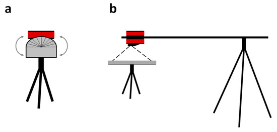
Figure 1.
Set-up for the experiments with the Sequoia camera and sunshine sensor mounted on a tripod. In (a), the sunshine sensor was mounted on a stand where the orientation was changed in 5° intervals around one axis and compared to a fixed photosynthetic active radiation (PAR) sensor. In (b), the camera was facing down over a 5% reflectance calibration panel to study the influence of sensor temperature on the sensitivity of the camera.
2.2.2. Studying the Influence of Camera Temperature on Sensor Corrected DN
To study the influence of camera temperature, the camera and the sunshine sensor were mounted on a bar fixed to a tripod with the camera facing a 5% Spectralon reflectance calibration panel (Labsphere, North Sutton, USA; Figure 1b). The 5% reflectance calibration panel was chosen to avoid saturation, and the camera was mounted without casting any shadow on the panel and with the reflectance calibration panel covering the entire image. Images were captured with 2 s intervals for 45 min in stable sunny conditions, and a PAR sensor was used to measure irradiance. Exposure calibration and vignetting correction (Section 2.3.2) were applied to the images, and mean pixel values for all images were calculated and plotted against irradiance from the PAR sensor to analyze if the relationship was linear for all camera temperatures. The camera temperature was derived from the image metadata.
2.2.3. Studying the Influence of Atmosphere on the Images
Three flights (Table 2) were performed in 2019 with the Sequoia camera mounted on a 3DR Solo multi-rotor UAS (3DR Robotics, California, USA). The flights were routine flights within Swedish Infrastructure for Ecosystem Science (SITES) Spectral with three Spectralon reflectance calibration panels (nominal reflectance: 5%, 20%, 50%) with a size of 25 × 25 cm used to derive the equation of the empirical line method.
Table 2.
List of flights used to study the influence of atmosphere.
The influence of the atmosphere was studied by capturing images of the reflectance calibration panels at different flying heights (Figure 2). The images were captured when ascending and descending vertically over the reflectance calibration panels to reduce the influence of viewing angles. Exposure calibration, vignetting correction, and irradiance normalization (Step 1 in Figure 3 and Section 2.3.2) were applied to the images. Mean pixel values of the reflectance calibration panels were derived with ENVI (Harris Geospatial Solutions Inc., Boulder, USA) by drawing polygons (regions of interest; ROIs) and computing statistics for the ROIs. Only pixels entirely inside the reflectance calibration panels were included since pixels at the edges of the panels are influenced by the surroundings.
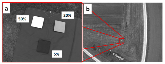
Figure 2.
Spectralon reflectance calibration panels (25 × 25 cm) in images captured at 1 m (a) and 55 m (b) flying heights during the flight on 20 May 2019. Both images are in the green wavelength band.
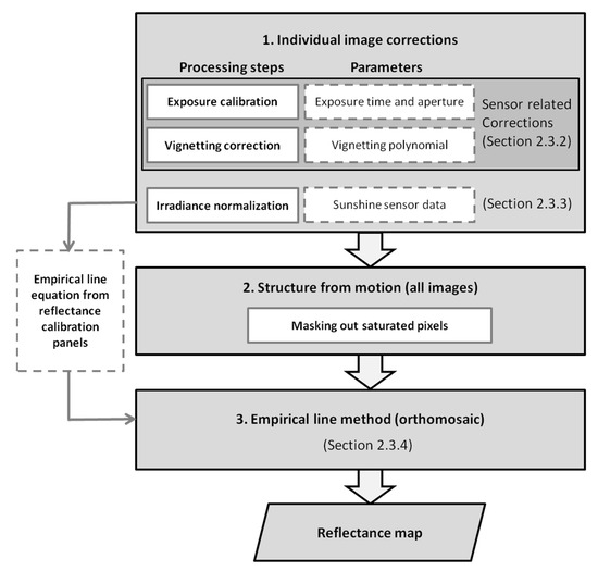
Figure 3.
Workflow of the radiometric correction method to create a reflectance map from Parrot Sequoia images. First, exposure calibration, vignetting correction, and irradiance normalization were performed on the individual images. Then, the images were processed with structure-from-motion techniques. Lastly, the empirical line method was applied to the orthomosaic to create a reflectance map. The equation for the empirical line method was derived from reflectance calibration panels in corrected individual images.
2.3. Image Processing
2.3.1. Overview of the Radiometric Correction Method
The workflow to perform radiometric correction is illustrated in Figure 3. First, the individual images were corrected with sensor specific corrections: exposure calibration (adjusting for different exposure settings) and vignetting correction as described in Section 2.3.2. Then irradiance normalization was applied to normalize the images for variability in irradiance (Section 2.3.3). The corrected images were then processed with structure from motion techniques to create an orthomosaic with all saturated pixels masked out. Lastly, the empirical line method was applied to the orthomosaic to create a reflectance map, i.e., an orthomosaic where the pixel values are converted to surface reflectance (Section 2.3.4). The equation for the empirical line method was derived from reflectance calibration panels in corrected individual images. For the experiments in Section 2.2, we only applied the individual image corrections. For the evaluation (Section 2.4), the entire workflow was applied to create a reflectance map.
2.3.2. Sensor-Related Correction of Individual Images
Exposure calibration and vignetting correction were performed on the individual images according to the methods described by Parrot [33,34] and with information derived from the image metadata (EXIF/XMP). All corrections were performed with in-house developed Python scripts.
Exposure calibration was performed to adjust for different exposure settings (exposure time and ISO value) in the individual images according to Equation (1) provided by Parrot [34].
where L is the at-sensor radiance in an arbitrary unit (homogeneous to W·s−1·m−2) common to all Sequoia cameras, f is the aperture f-number (f = 2.2 for Sequoia), DN is the digital number of a pixel, ε is the exposure time, γ is the ISO value, and A, B, C are calibration coefficients provided in the image metadata.
Vignetting is the radial decrease in pixel values which results in darker areas near the edges of images [12]. In this study, the vignetting correction was performed by dividing the exposure-calibrated images with the vignetting polynomial, where the polynomial was derived from the EXIF/XMP metadata of the Sequoia images. The vignetting polynomial is estimated with the flat field method [33]; a large number of images are captured over a surface with Lambertian reflectance properties to find the correction factor for each pixel, and a polynomial is fit to the pixel-wise correction factors (e.g., [19,41]).
2.3.3. Irradiance Normalization of Individual Images
Irradiance normalization was performed on the individual images after exposure calibration and vignetting correction. However, the raw irradiance data from the sunshine sensor were noisy and sensitive to sensor orientation (yaw, pitch, roll) since they did not have a cosine corrector. Hence, polynomials or splines were fitted to smooth the raw sunshine sensor data, and the value of the polynomial or spline, from here on called smoothed irradiance, was used to normalize the images instead of the raw data. Figure 4 shows raw sunshine sensor data and fitted splines in cloudy conditions, i.e., with mainly diffuse light (a, c), and raw sunshine sensor data and a fitted polynomial in mainly sunny conditions with thin clouds, i.e., with mainly direct light (b), where the variability correlates with flight direction. The polynomial and splines were manually fitted to the data, and the best fit was selected on the basis of a visual inspection. The image-specific irradiance normalization factor (Cin,i; Equation (2)) was then calculated for each image.
where Cin,i is the irradiance normalization factor for image i, I(λ) is the mean smoothed irradiance for wavelength band λ for all images in a flight, and Ii(λ) is smoothed irradiance from the sunshine sensor for image i. The irradiance normalization was then performed by dividing all pixels in an image with the image specific normalization factor (Cin,i). To minimize the normalization factor and avoid large modification of images, all images were normalized against the mean smoothed irradiance for the entire flight.
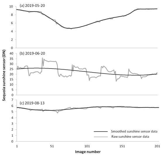
Figure 4.
Raw sunshine sensor data (gray) and smoothed sunshine sensor data (black) for the flights on 20 May 2019 (a), 20 June 2019 (b), and 13 August 2019 (c).
2.3.4. Creating Reflectance Maps with the Empirical Line Method
A reflectance map was created from the images collected during a flight on 22 September 2020 (Section 2.4) to evaluate the workflow in Figure 3. The individual images were corrected as described in Section 2.3.2 and Section 2.3.3, and then processed in Agisoft Metashape ver. 1.6.5 to create an orthomosaic.
A common problem of the Sequoia camera is the occurrence of saturated pixels [25,39]. In this study, saturated pixels were found across several images, especially in the green and red wavelength bands. Usually, the saturated pixels were over bright areas, such as gravel or rocks, which are not interesting for vegetation monitoring. To avoid the influence of saturated pixels on the orthomosaics, a mask was created for each image to mask out the saturated pixels when creating the orthomosaic. The masks were created with the in-house Python script that performed the radiometric correction of the individual images, in a format that enabled direct import into Agisoft Metashape. No radiometric correction was performed in Agisoft Metashape except for the blending mode being applied when creating the orthomosaic. The blending mode separates the data into frequency domains; along the seamlines, all frequencies are blended, while only lower frequencies are blended with increasing distance from seamlines [42]. The orthomosaic was exported from Agisoft Metashape with a spatial resolution of 5.5 cm, and the empirical line method [11] was applied to convert the DN of the orthomosaic to surface reflectance according to Equation (3).
where R is the reflectance, DNcorr is the radiometrically corrected DN value after applying exposure calibration, vignetting correction, and irradiance normalization, a is the slope of the regression line, and b is the intercept (Figure 5).
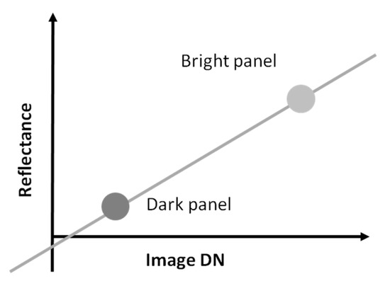
Figure 5.
Illustrating how the equation for the empirical line method is derived from one dark and one bright reflectance calibration panel to get the slope (a in Equation (3)) and the intercept (b in Equation (3)) of the empirical line. In this study, two or three panels were used to derive the equation.
The equation for the empirical line method was derived from individual, radiometrically corrected images. Since the results indicate that there is an influence of the atmosphere on the images (Section 3.3), mean pixel values over reflectance calibration panels were derived from an image recorded as close to the maximum flying height as possible. It is, however, important that the pixels used to estimate the mean values are entirely inside the reflectance calibration panels and do not include mixed pixels near the edges of the panels that are influenced by the surroundings. Hence, it is a tradeoff between obtaining a more robust mean from a larger number of pixels and deriving the mean values from images near the flying height (see Figure 2 for a comparison between the Spectralon reflectance calibration panels at flying heights of 1 m and 55 m during the flight on 20 May 2019). For the flight on 22 September 2020, images captured at 28 m flying height were used to derive mean pixel values. For higher heights, saturated and mixed pixels limited the number of available pixels to derive mean values.
In all flights, the pixels of the 50% reflectance calibration panels were saturated in the green and red wavelength bands. Hence, the equation for the empirical line was derived from two panels only for these bands. For the red-edge and near-infrared bands, there was no saturation, and all three reflectance calibration panels could be used to derive the equations. Since reflectance for vegetation is around 5–10% in the green and red wavelength bands, the range is well covered by the 5% and the 20% reflectance panels, and the equation for the empirical line can be estimated without the 50% reflectance panel.
2.4. Evaluation with Field Spectral Data
To evaluate the accuracy of the reflectance map, a comparison was done between reflectance and NDVI obtained with the suggested radiometric correction method and reflectance and NDVI from spectral field measurements. The evaluation was performed with data from an experimental flight on 22 September 2020 at 2:30 p.m. The flight was conducted in thin cloud cover at a flying height of 60 m, and two sets of Spectralon reflectance panels were used. The spectral field reflectance measurements were performed with a handheld Apogee PS-100 spectroradiometer (Apogee Instruments, Inc., Logan, Utah, United States) calibrated against an Apogee AS-004 97% white reflectance panel (Apogee Instruments, Inc., Logan, UT, United States). Field reflectance was measured over nine spectral field plots (1 × 1 m) with short green grass (Figure 6a), green sugar beets (Figure 6b), and dry wheatgrass (Kernza; Figure 6c), to cover a range of NDVI values (Table 3). The spectral field plots were marked with plastic ribbons to identify them in the UAS images. A series of spectral measurements were conducted over the field plots (2–7 per plot) during the period 10:45 a.m.–1:45 p.m. For each measurement, three spectral measurements were collected per plot, where each measurement was averaged over five spectral samples. The reflectance was measured at a resolution of 1 nm in the spectral range of 339–1177 nm, and an integration time of 20–25 ms depending on light conditions. The spectroradiometer was held approximately 0.5 m above each plot when collecting the measurements. Calibration against the white reflectance standard was made every sixth reading. Measurements obtained outside the range of 400–1000 nm were removed due to a low signal-to-noise ratio.
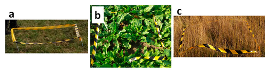
Figure 6.
Three of the spectral field plots with green grass (a), green sugar beets (b), and dry wheatgrass (c).
Table 3.
Overview of the spectral field plots.
2.4.1. Parrot Sequoia Data
Mean reflectance for the four wavelength bands of the Sequoia camera was derived for the nine spectral field plots with ENVI. In addition, NDVI was calculated from the reflectance map according to Equation (4).
where Rred and RNIR are the reflectance for the Sequoia red and near-infrared wavelength bands, respectively. Lastly, mean NDVI values for the nine spectral field plots were obtained.
2.4.2. Spectral Field Data
Since the spectral response functions for the wavelength bands of the Sequoia camera are not known, reflectance for the four bands was calculated from the field spectral data as the mean reflectance for the spectral ranges of the Sequoia wavelength bands (Table 1), i.e., assuming a uniform response within the wavelength bands. In addition, NDVI was calculated from the field spectral data according to Equation (4). Lastly, regression analyses were performed to find the correlations and biases between the Sequoia-derived data and the field spectral data, where the field spectral data were considered more accurate and, hence, used as evaluation data.
3. Results
3.1. Performance of the Sunshine Sensor
The Sequoia sunshine sensor data from the first experiment (Section 2.2.1) showed a similar response to variability in irradiance as the factory-calibrated Skye sensor in both the red (Figure 7) and the red-edge wavelength bands. The actual values could not be directly compared since the Sequoia sunshine sensor data were in an arbitrary unit common to all Sequoia cameras, but the linear correlation between the two sensors was strong with R2 = 0.998 for both the red (Figure 7b) and the red-edge wavelength bands. The strong linear correlations indicate that data from the Sequoia sunshine sensor are sufficiently accurate to perform irradiance normalization, and, since a ratio is used to perform irradiance normalization, the unit is not important.
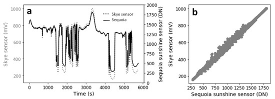
Figure 7.
Comparison between Sequoia sunshine sensor data (red wavelength band) and irradiance measured with a factory-calibrated Skye sensor (a) and correlation between Sequoia sunshine sensor data and Skye sensor data (b). -R2 = 0.998.
The results from the experiment when the sunshine sensor was tilted around one axis show that the cosine-corrected sunshine sensor data agreed well with irradiance from the horizontally mounted PAR sensor for lower tilt angles. Figure 8 shows the cosine-corrected irradiance from the sunshine sensor in the green wavelength band (brown line) and PAR from the upward-looking PAR sensor (beige line) when the sunshine sensor was tilted around the roll axis in 5 min intervals. Since irradiance from the sunshine sensor was in an arbitrary unit, the PAR sensor data were scaled to irradiance from the sunshine sensor when it was horizontally oriented at the initial stage of the experiment. When the sunshine sensor was tilted toward the south (decreasing incidence angle; black line), the cosine-corrected irradiance from the sunshine sensor stayed close to PAR until the roll (gray line) was 20° (Figure 8a). When the sunshine sensor was rotated toward the north (increasing incidence angle; black line), the cosine-corrected irradiance from the sunshine sensor stayed close to PAR until the roll (gray line) reached 25° (Figure 8b). It should be noted that, for larger tilt angles, the hemispherical view of the tilted sunshine sensor would include sections of the roof on which it was placed during the experiment and surrounding buildings, which would influence the measurements. Hence, the data are not be comparable to the PAR sensor which was horizontally mounted during the experiment. Furthermore, during the flight, the roll and pitch angles of the sunshine sensor stayed well below 20°.
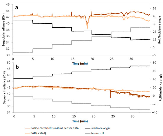
Figure 8.
Cosine-corrected irradiance in the green wavelength band from the sunshine sensor (brown) and PAR (beige) measured with a horizontally mounted PAR sensor. Incidence angle for the sunshine sensor is shown in black and the roll is shown in gray. The sensor was rotated toward the south (decreasing incidence angles) in (a) and toward the north (increasing incidence angles) in (b). Data were collected in sunny conditions.
However, even though the experiments indicated that the sunshine sensor is accurate, it was noted that the IMU in the sensor does not give accurate orientation (roll, pitch, and yaw) during flights. Figure 9 shows the roll, pitch, and yaw angles for the four flight tracks during the flight on 22 September 2020. The log file from the 3DR Solo showed that the roll, pitch, and yaw for the UAS were stable within 2–3° along a flight track (see Supplementary Materials), while the sunshine sensor IMU recorded differences of 5–10° for roll and pitch and 30–40° for yaw. The noisy orientation data make it difficult in practice to perform an accurate cosine correction of the sunshine sensor data.
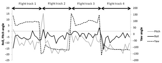
Figure 9.
Roll, pitch, and yaw for the sunshine sensor during the flight at Lönnstorp on 22 September 2020.
3.2. Influence of Camera Temperature on Sensor Corrected DN
There was a strong linear relationship between irradiance (PAR) and sensor corrected DN values of the reflectance calibration panel for all bands once the camera warmed up. However, for lower camera temperatures, the relationship was strongly nonlinear (Figure 10). The results show that the sensitivity of the camera is influenced by temperature and that it is important to let the camera warm up before starting to collect data, especially if an image of a reflectance calibration panel is captured early during the flight and used to derive the equation for the empirical line method.
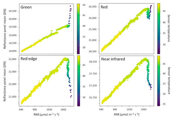
Figure 10.
Relationship between exposure-calibrated and vignetting-corrected digital number (DN) values and irradiance (PAR). For lower camera temperatures, the relationship was strongly nonlinear; however, once the camera warmed up, the relationship became linear.
The analysis did not reveal any consistent number of images required for the camera to warm up before the relationship became linear. When the camera was mounted on a tripod, the temperature became stable for all wavelength bands after around 200 images (100 s) when the camera reached a temperature of just less than 50 °C (see Figure 11 for the green and red bands; the other bands behaved in a similar fashion but are omitted in the figure for the sake of legibility). The linear relationship between PAR and reflectance calibration panel mean values (Figure 10) was reached at around 47 °C for the near-infrared and red-edge bands after just over 200 images (Table 4). For the green band, the relationship became linear at just 33 °C and 17 images (Table 4), but there was a shift in the relationship at a temperature around 47.5 °C after around 390 images for the green band (Figure 10) that was not present in the other wavelength bands.
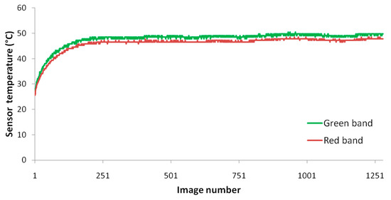
Figure 11.
The camera temperature stabilized at just less than 50 °C after around 200 images for the green and red wavelength bands when it was mounted on a tripod (Figure 1b). The red-edge and near-infrared bands behaved in a similar fashion but are omitted in the figure for the sake of legibility.
Table 4.
Sequoia camera temperature when the relationship between PAR and reflectance calibration panel mean values became linear (Figure 10) and the number of images captured when the temperature was reached.
However, during a flight, the camera temperature does not always stabilize due to, e.g., cooling effects from the wind. Figure 12 shows the Sequoia sensor temperature for the green band during the three flights at Lönnstorp in 2019 (Table 2). The temperature increased rapidly when the camera started capturing images; however, for the flight on 20 June, in sunny conditions with only thin clouds, the temperature stabilized faster than for the two flights in cloudy conditions, which might have had an influence on the images captured.
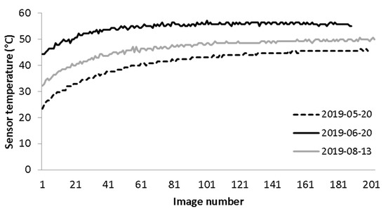
Figure 12.
Sequoia sensor temperature for the green band during the flights in 2019 (Table 2).
3.3. Influence of Atmosphere
The results from the three flights in Lönnstorp in 2019 indicate that the atmosphere has an influence on the images. Figure 13, Figure 14 and Figure 15 show mean DN values over the reflectance calibration panels at different flying heights for the green, red, and near-infrared wavelength bands during the flight on 20 May 2019 in cloudy conditions. In the figures, images captured when descending over the reflectance calibration panels were used, since camera temperature was stable in the later part of the flight (panel b in the figures). Irradiance was also stable during the descent (see panel c in the figures for smoothed sunshine sensor data), and images with the reflectance calibration panels in the central parts of the images were selected to reduce the influence of factors other than flying height. For the red and green wavelength bands, the pixels over the 50% reflectance calibration panel were saturated in all images. For the green and red wavelength bands, some images were also saturated over the 20% reflectance panels, and, for some flights, all images over the 20% reflectance calibration panel were saturated in the green wavelength band during descent. There were generally more saturated pixels during descent when the camera was warmer.
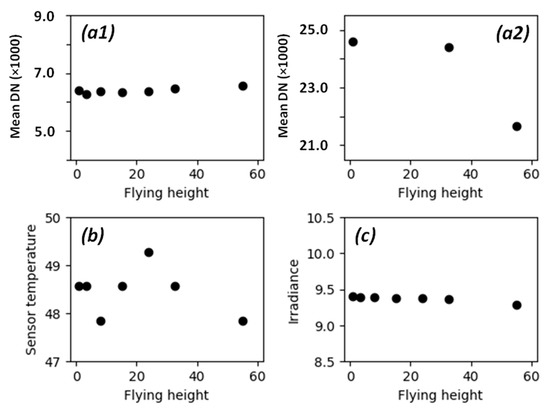
Figure 13.
Mean pixel values for the green band over the 5% (a1) and the 20% (a2) reflectance calibration panels during the flight on 20 May 2019. The low number of observations for the 20% panel was due to saturation in some images. Images were captured while descending over the panels with stable camera temperature (b) and irradiance (c).
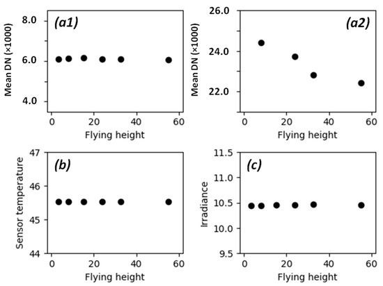
Figure 14.
Mean pixel values for the red band over the 5% (a1) and the 20% (a2) reflectance calibration panels during the flight on 20 May 2019. The low number of observations for the 20% panel was due to saturation in some images. Images were captured while descending over the panels with stable camera temperature (b) and irradiance (c).
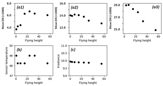
Figure 15.
Mean pixel values for the near infrared band over the 5% (a1), the 20% (a2), and the 50% (a3) reflectance calibration panels during the flight on 20 May 2019. Images were captured while descending over the panels with stable camera temperature (b) and irradiance (c).
The radiometrically corrected pixel values for the 5% reflectance calibration panel increased slightly with flying height for the green wavelength band. For the near-infrared band, the pixel values were higher for higher flying heights with a shift to higher values at around 15 m height. The red band appeared to be stable over the different flying heights for the 5% panel. For the 20% and the 50% reflectance calibration panels, on the other hand, the pixel values decreased with flying height for all wavelength bands. The results were similar for the other two flights in 2019 (see Supplementary Materials).
The numbers of pixels used to derive mean pixel values and standard deviation in the near-infrared band for the flight on 20 May 2019 are presented in Table 5. The magnitude of the standard deviation was largest for the 5% reflectance calibration panel, indicating that there was more noise in the panels with lower reflectance. The other wavelength bands showed the same pattern. Since there is a direct relationship between flying height and pixel size, the number of pixels used to derive the statistics decrease with increasing flying height. However, since the pixels used to derive the mean values must be entirely inside the reflectance calibration panels, the number of pixels was not the same for all panels at the same flying height.
Table 5.
Mean pixel values and standard deviation for the reflectance calibration panels at different Figure 15. “Nbr pixels” denotes the number of pixels used to derive mean and standard deviation for the different flying heights.
3.4. Evaluation against Field Spectral Data
The Parrot Sequoia images from the experimental flight in 2020 were radiometrically corrected, and a reflectance map was created according to the workflow in Section 2.3 (Figure 3). Figure 16 shows the central part of the reflectance map as a color infrared (CIR) map with enlargements over spectral field sample areas for green sugarbeet (a), green grass (b), and dry wheatgrass (c). The spectral field plots are marked with black squares, with only two of the five plots covered in the sugarbeet field included in the enlargement.
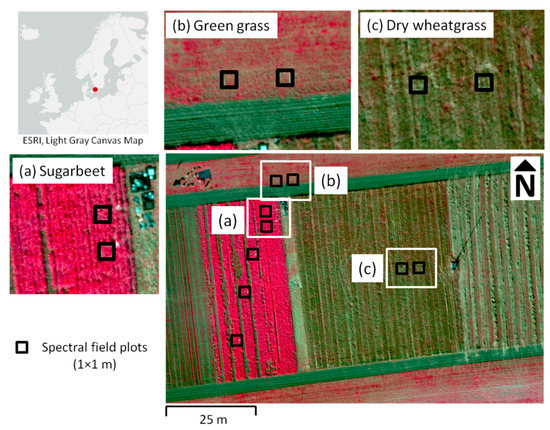
Figure 16.
Color infrared reflectance map over the central part of the flight over Lönnstorp research station in south Sweden on 22 September 2020. The spectral field plots are marked with black squares with enlargements over two spectral field plots for green sugarbeet (a), green grass (b), and dry wheatgrass (c).
The temperature of the Sequoia camera was stable during the flight, ranging from 53–55°C for the images included in the reflectance map (Figure 17). Reflectance panel mean values were obtained from image #131 at a temperature of 53 °C.
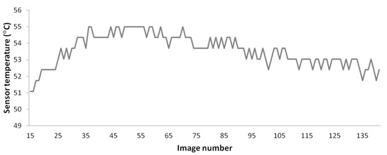
Figure 17.
Temperature of the Sequoia camera during the flight on 22 September 2020. Images captured before takeoff are not included. The camera reached a temperature of 54 °C before the first image included in the reflectance map was captured.
The four spectral bands in the reflectance map were evaluated against field spectral data collected over the nine spectral field plots. Figure 18 and Table 6 show the correlation between reflectance from the Sequoia camera and the field spectral data. Reflectance from the Sequoia camera was slightly lower than reflectance from the field spectral measurement for all four wavelength bands. Correlation was highest for the red wavelength band (R2 = 0.97) followed by the near-infrared (R2 = 0.84) and the red-edge (R2 = 0.80) bands. The green band had the lowest correlation (R2 = 0.39), but the range of reflectance values for the field sampling areas was narrow for the green band (7.7–11.4% from field spectral data) compared to the other wavelength bands, highlighting that the uncertainty of the measurements has a stronger impact on the results.
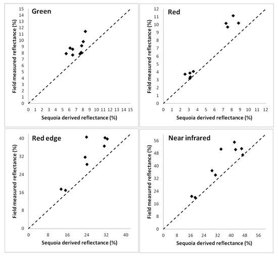
Figure 18.
Correlation between the reflectance map (Sequoia) and field spectral data for the nine spectral field plots. Green band R2 = 0.39, red band R2 = 0.97, red-edge band R2 = 0.80, and near-infrared band R2 = 0.84.
Table 6.
Equation and R2 for the regression between reflectance from the Sequoia camera and the field spectral measurements, where y is the field spectral data and x is Sequoia reflectance. NDVI, normalized difference vegetation index.
The high correlation for the red and near-infrared bands, with both bands slightly underestimating reflectance compared to the field spectral data, resulted in accurate NDVI values. For the red wavelength band, with a negative intercept and a slope of 1.33 (Table 6, Figure 18), the Sequoia-derived reflectance agreed best with the field spectral data for lower reflectance values. This implies that the accuracy is highest for healthy vegetation. For the near-infrared wavelength band, with an intercept of 3.85 and a slope of 1.09, there was a more stable bias with lower reflectance values for the Sequoia data for the entire range of reflectance values. This resulted in the highest accuracy of NDVI for healthy vegetation, i.e., with high NDVI values. This is shown in Figure 19, where the correlation between NDVI from the Sequoia camera and the field spectral measurement gave R2 = 0.99, with a slightly overestimated NDVI from the Sequoia camera for lower NDVI values.
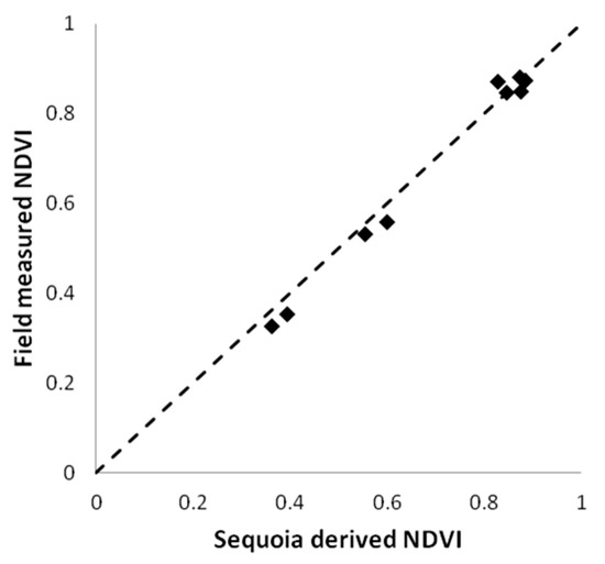
Figure 19.
Correlation between NDVI from the Sequoia camera and NDVI from the field spectral data for the nine spectral field plots. R2 = 0.99.
4. Discussion
This study presented a workflow to perform radiometric correction of images collected with the Parrot Sequoia camera (Figure 3). The workflow is similar to that suggested by Parrot [33,34,43], and to earlier studies where different radiometric calibration methods for the Sequoia camera were compared [11,24,38,39]. However, in this study, we performed experiments that gave valuable information about the performance of the Sequoia camera and sunshine sensor that might explain the inconsistencies in earlier studies. The main findings related to image collection were that the sensitivity of the camera is influenced by camera temperature and that there is an influence of the atmosphere on the images. The main difference related to image processing compared to earlier studies is the way we handled noise in the raw sunshine sensor data.
The temperature dependency implies that it is important to let the camera warm up before starting to capture images that will be used for processing. This is especially important if reflectance calibration images are captured before the flight. It is, however, difficult to state how long the camera needs to warm up, and there will be a tradeoff between flying time and warming up the camera if the Sequoia is connected to the UAS battery. We suggest letting the camera warm up for at least 1 min before starting the UAS and taking off; however, the precise time will depend on ambient temperature and wind.
The results indicated that there was an influence of the atmosphere and that corrected DN values decrease with flying height for the 20% and 50% reflectance calibration panels. This could be due to the increasing water absorption with increasing atmospheric depth, but the variability in the results makes it hard to draw any conclusions. For the 5% reflectance calibration panel, the results showed the opposite trend with increasing pixel values with increasing flying height, especially for the near-infrared band, where the largest increase in pixels values occurred at lower flying heights. For the green and red wavelength bands, the influence of flying height seemed to be low for the 5% reflectance calibration panel. The different trends for darker and brighter reflectance calibration panels are hard to explain. It should, however, be noted that it is not only the depth of the atmosphere that is influenced by flying height. The spatial resolution of the pixels increases with flying height, and larger areas of the ground around the reflectance panels will be included in the images. The spectral properties, e.g., darker versus brighter ground cover, of the areas surrounding the reflectance panels might also influence the pixel values over the panels. Stow et al. [11] also studied the influence of flying height with a Parrot Sequoia camera and found a weak increasing trend with increasing flying height for some flights, but the results varied between flights, and not all flights showed this effect. The studied reflectance values were in the range 4–8%, which agrees with the results of our study for the 5% reflectance calibration panel. The authors also found a larger impact in the red-edge and near-infrared bands compared to green and red. Guo et al. [23] studied the atmospheric effect on images captured by the Mini MCA 6 multispectral camera by estimating the empirical line equation for individual images captured at different flying heights and comparing the intercept of the x-axis. The authors found an increasing trend with height but the influence on reflectance was low (1.5% at 100 m). There are also studies where atmospheric modeling was applied to estimate and correct for the influence of the atmosphere on images collected with UASs [44,45]. However, during the relatively short flying time of a UAS, the atmosphere is rather stable; hence, if images of reflectance calibration panels are captured at elevations close to flying height, the empirical line method can be applied to correct for the atmospheric influence.
To ensure that the influence of the atmosphere is similar on the images used to derive the equation for the empirical line method and the images used to create the orthomosaic, we suggest ascending and descending over the reflectance calibration panels at the beginning and just after the mission. This will enable capturing images of the reflectance calibration panels close to the flying height of the actual mission. It will also produce a large number of images of reflectance panels, which increase the chance of avoiding saturated pixels, as well as balance the tradeoff between having images of reflectance calibration panels captured at higher flying heights and the number of pure pixels over the panels. Another option to increase the number of pure pixels when estimating the equation for the empirical line method at higher flying heights is to use larger reflectance calibration panels. In this study, we used 25 × 25 cm panels, which make it difficult to get enough pure pixels at flying heights over 60 m with the Sequoia camera. Larger reflectance calibration panels, such as the 1 × 1 m panels used by [31,32], would substantially increase the number of pure pixels and enable estimates of mean reflectance at higher flying heights.
We also suggest using a larger number of reflectance calibration panels with reflectance lower than 20% to have more reflectance values to derive the equation for the empirical line method. In this study, we used reflectance calibration panels with 5%, 20%, and 50% nominal reflectance; however, for the green and red wavelength bands, there were in some cases saturated pixels in both the 20% and the 50% reflectance panels. Even though there were images with at least both 5% and 20% available, there were many images at higher flying heights with saturation in the 20% reflectance panel. With more panels with lower reflectance, there would be a higher chance of getting images with at least two reflectance calibration panels without saturation at higher flying height. In addition, a larger number of reflectance calibration panels would give an indication if the relationship between the corrected DN values of the images and surface reflectance is linear. However, larger and more reflectance calibration panels would mean additional equipment to bring to the field, and high-quality reflectance calibration panels, such as Spectralon used in this study, come with a high cost. Furthermore, it is crucial to handle reflectance calibration panels with care and maintain them to avoid damage and surface degradation. Assman et al. [10] found reductions in reflectance of 4–10% in reflectance calibration panels during a 3 month period in a harsh environment (Arctic tundra).
The problem with saturated pixels indicates that the camera cannot adequately handle large contrast in the scenes captured in an image. Usually, the saturated pixels are over bright areas, such as reflectance calibration panels with high reflectance, gravel, or rocks, which cover only a small fraction of an image where the ground cover is generally dark. For vegetation monitoring, rock and gravel are less interesting, and we consider the pixels without saturation reliable in images with saturation. Even though the 20% reflectance calibration panel was saturated in the green and red wavelength bands in several images, vegetation generally had a reflectance of 5–10%, which is well below 20% and should, hence, not be influenced by the saturation.
The results show that the sunshine sensor is accurate; however, since the sensor does not have a cosine corrector, the data are influenced by sensor orientation, which introduces noise into the data. Hence, the raw sunshine sensor data need to be smoothed before irradiance normalization is performed. In this study, noise in the sunshine sensor data was handled by fitting functions to the raw data. A disadvantage with the method is that there is no objective method to find the best fit of the function, and some trial and error is needed to find a satisfactory result. Another option would be to measure irradiance with a ground-based sensor during the flight [28,29]. This would give more accurate irradiance data than if the sunshine sensor is mounted on the UAS, but with the disadvantage that more equipment would be required to bring to the field, and the set-up for a flight would be more complicated.
Mosaic blending mode was used in this study when creating the orthomosaic in Agisoft Metashape. Berra et al. [19] suggested using disabled blending mode when creating orthomosaics to avoid any modification of pixel values. With blending mode disabled, a pixel in the orthomosaic gets the value of the original image that is closest to the surface normal of the pixel in the orthomosaic [42]. However, for the experimental flight in 2020, there were images with saturated pixels in the near-infrared band over the sugarbeet parcel. When the saturated pixels are masked out, the pixel values in the orthomosaic are derived from UAS images further from the surface normal of the orthomosaic, which can result in larger differences in pixels values between neighboring pixels if blending is disabled. Hence, mosaic blending mode was used to reduce the influence of the gaps caused by saturated pixels that were masked out. The reason for the saturation in some images was that the parcel with green sugarbeet had much higher reflectance in the near-infrared band compared to the surroundings with no or little vegetation; hence, the camera could not fully handle the large contrasts. In areas with more homogeneous vegetation, it might be an option to disable blending mode since saturation does notusually appear in the near-infrared band.
In sunny conditions, there is a strong influence of viewing and illumination angles on the individual images (e.g., [7,11,25]) with the main influence in the hotspot region where illumination and viewing angles coincide [46]. No corrections for these bidirectional reflectance distribution function (BRDF) effects were performed in this study. Studies that modeled the BRDF with high accuracy were conducted over more homogeneous agricultural fields with single crops (e.g., [32,47,48,49]). Over such homogeneous fields with similar spectral properties, it is comparatively easy to find a large number of observations with different viewing and illumination angles in the images without considering the ground cover. In more complex landscapes, with higher variability in spectral properties between different land-cover types, it is harder to model the BRDF. Tu et al. [25] performed a BRDF correction of Sequoia images over avocado and banana plantations; however, for the complex shapes of the tree canopies, the BRDF model did not perform well, which was also found by Näsi et al. [31] in hyperspectral data over forests. The experimental fields in Lönnstorp, where data were collected for this study, are relatively small (generally 25 × 50 m parcels) and with different crop types in various growth stages mixed with nonvegetated areas. This heterogeneity makes it very difficult to model the BRDF. Furthermore, the main focus was to fly in cloudy conditions to avoid strong BRDF effects. However, it is important to be aware of the BRDF effects when flying in sunny conditions.
Earlier studies showed that it is difficult to find a single method that gives the best result when performing radiometric correction of Parrot Sequoia images. Poncet et al. [39] compared different methods to perform radiometric correction of Parrot Sequoia images and found that no method resulted in the lowest accuracy for all bands; however, they suggested performing the empirical line method on the processed orthomosaic rather than on the raw images. Tu et al. [25] conducted a similar study over avocado and banana plantations and found that none of the radiometric correction methods tested performed consistently better in all flights performed. Stow et al. [11] found generally higher reflectance values in images captured during ascent compared to images captured during descent; this difference might be due to differences in sensor sensitivity since the camera is usually warmer in the later part of a flight. This study provided some approaches to compensate for some of the uncertainties by considering the influence of camera temperature and atmosphere on the individual images, as well as reducing the influence of noise in the sunshine sensor data. Our results also showed that the accuracy of NDVI is higher than the accuracy of reflectance of the individual bands. This is expected since one advantage with NDVI and other normalized vegetation indices is that they are more robust against illumination differences [50]. Franzini et al. [38] and Stow et al. [11] also found that deviations were larger for Sequoia-derived reflectance than NDVI, and that NDVI seemed to behave better than other tested vegetation indices [38]. Hence, we suggest using normalized vegetation indices rather than reflectance when performing quantitative analyses using imagery collected from UASs with consumer-type multispectral cameras.
5. Conclusions
In this study, we conducted experiments that give valuable information about the performance of the Parrot Sequoia camera and associated sunshine sensor. The results showed that the camera must become sufficiently warm before the sensitivity of the sensor becomes stable. Hence, it is important to let the camera warm up before capturing images of reflectance calibration panels and starting to collect data.
The results also indicated that the atmosphere influences the images captured from a UAS. Hence, we suggest ascending and descending over reflectance calibration panels at the beginning and just after the mission to capture images over the panels near the maximum flying height. This will give images of the reflectance calibration panels with the same atmospheric depth as the images captured during the actual mission. It will also give a large number of images with reflectance calibration panels, which will decrease the risk of having saturation over panels when estimating the equation for the empirical line correction. In this study, we used 25 × 25 cm reflectance calibration panels with 5%, 20%, and 50% nominal reflectance. We suggest using larger panels to get more pure pixels over the panels at higher flying heights. We also suggest using more panels with different reflectance lower than 20% to avoid the risk of saturation and to get a more robust estimate of the equation for the empirical line method.
The results showed that the sunshine sensor performs well. However, since the sunshine sensor does not have a cosine corrector, it is sensitive to orientation and the motions of the UAS, which results in noisy data. To handle the noise in the sunshine sensor data, we fit smoothing functions to the raw data and used the smoothed data to perform irradiance normalization.
With the workflow suggested in this study, we achieved an R2 of 0.99 when evaluating the Sequoia-derived NDVI with NDVI from field spectral measurements. For the individual wavelength bands, R2 was 0.80–0.97 for the red-edge, near-infrared, and red bands but low (0.39) for the green band. Hence, the study showed that NDVI can be derived with high accuracy with the Parrot Sequoia camera, and we suggest using normalized vegetation indices rather than reflectance when performing quantitative analyses using imagery collected from UASs with consumer-type multispectral cameras.
Supplementary Materials
The following are available online at https://www.mdpi.com/2072-4292/13/4/577/s1, Figure S1: Mean pixel values for the green band over the 5% (a) reflectance calibration panels during the flight on June 20, 2019. Images were captured while descending over the panels with stable camera temperature (b) and irradiance (c).
Author Contributions
Conceptualization, P.-O.O., L.E., K.A., and V.E.G.M.; methodology, P.-O.O. and K.A.; software, P.-O.O. and K.A.; formal analysis, P.-O.O., A.V., and K.A.; investigation, P.-O.O., A.V., K.A., A.K., and M.A.; writing—original draft preparation, P.-O.O.; writing—review and editing, P.-O.O., L.E., and V.E.G.M.; visualization, P.-O.O.; funding acquisition, L.E. All authors have read and agreed to the published version of the manuscript.
Funding
This investigation was carried out with support from the SITES Spectral Thematic Center. SITES receives funding through the Swedish Research Council under the grant no 2017.00635. It was also supported by the Swedish Research Council FORMAS project CarboScale, grant 2016-01223 to Lars Eklundh. We acknowledge support from the Nordforsk project NordPlant, grant 84597.
Data Availability Statement
No new data were created or analyzed in this study. Data sharing is not applicable to this article.
Acknowledgments
We thank the SITES Lönnstorp Research Station for access to their field research area and facilities and Ryan Davidson for performing the 2019 flights within SITES Spectral. Hongxiao jin and Marcin Jackowicz-Korczynski, Department of Physical Geography and Ecosystem Science, Lund University, are acknowledged for assistance during experiments and with equipment maintenance.
Conflicts of Interest
The authors declare no conflict of interest.
References
- Singh, K.K.; Frazier, A.E. A meta-analysis and review of unmanned aircraft system (UAS) imagery for terrestrial applications. Int. J. Remote Sens. 2018, 39, 5078–5098. [Google Scholar] [CrossRef]
- Simic Milas, A.; Sousa, J.J.; Warner, T.A.; Teodoro, A.C.; Peres, E.; Gonçalves, J.A.; Delgado Garcia, J.; Bento, R.; Phinn, S.; Woodget, A. Unmanned Aerial Systems (UAS) for environmental applications special issue preface. Int. J. Remote Sens. 2018, 39, 4845–4851. [Google Scholar] [CrossRef]
- Zarco-Tejada, P.J.; Berni, J.A.J.; Suárez, L.; Fereres, E. A new era in remote sensing of crops with unmanned robots. SPIE Newsroom 2008. [Google Scholar] [CrossRef]
- Zhang, C.; Kovacs, J.M. The application of small unmanned aerial systems for precision agriculture: A review. Precis. Agric. 2012, 13, 693–712. [Google Scholar] [CrossRef]
- Radoglou-Grammatikis, P.; Sarigiannidis, P.; Lagkas, T.; Moscholios, I. A compilation of UAV applications for precision agriculture. Comput. Netw. 2020, 172, 107148. [Google Scholar] [CrossRef]
- Torresan, C.; Berton, A.; Carotenuto, F.; Di Gennaro, S.F.; Gioli, B.; Matese, A.; Miglietta, F.; Vagnoli, C.; Zaldei, A.; Wallace, L. Forestry applications of UAVs in Europe: A review. Int. J. Remote Sens. 2017, 38, 2427–2447. [Google Scholar] [CrossRef]
- Aasen, H.; Honkavaara, E.; Lucieer, A.; Zarco-Tejada, P.J. Quantitative Remote Sensing at Ultra-High Resolution with UAV Spectroscopy: A Review of Sensor Technology, Measurement Procedures, and Data Correction Workflows. Remote Sens. 2018, 10, 1091. [Google Scholar] [CrossRef]
- Manfreda, S.; McCabe, M.F.; Miller, P.E.; Lucas, R.; Pajuelo Madrigal, V.; Mallinis, G.; Ben Dor, E.; Helman, D.; Estes, L.; Ciraolo, G.; et al. On the Use of Unmanned Aerial Systems for Environmental Monitoring. Remote Sens. 2018, 10, 641. [Google Scholar] [CrossRef]
- Westoby, M.J.; Brasington, J.; Glasser, N.F.; Hambrey, M.J.; Reynolds, J.M. Structure-from-Motion photogrammetry: A low-cost, effective tool for geoscience applications. Geomorphology 2012, 179, 300–314. [Google Scholar] [CrossRef]
- Assmann, J.J.; Kerby, J.T.; Cunliffe, A.M.; Myers-Smith, I.H. Vegetation monitoring using multispectral sensors—Best practices and lessons learned from high latitudes. J. Unmanned Veh. Syst. 2018, 7, 54–75. [Google Scholar] [CrossRef]
- Stow, D.; Nichol, C.J.; Wade, T.; Assmann, J.J.; Simpson, G.; Helfter, C. Illumination Geometry and Flying Height Influence Surface Reflectance and NDVI Derived from Multispectral UAS Imagery. Drones 2019, 3, 55. [Google Scholar] [CrossRef]
- Goldman, D.B. Vignette and Exposure Calibration and Compensation. IEEE Trans. Pattern Anal. Mach. Intell. 2010, 32, 2276–2288. [Google Scholar] [CrossRef]
- Smith, G.M.; Milton, E.J. The use of the empirical line method to calibrate remotely sensed data to reflectance. Int. J. Remote Sens. 1999, 20, 2653–2662. [Google Scholar] [CrossRef]
- Honkavaara, E.; Markelin, L.; Hakala, T.; Peltoniemi, J. The Metrology of Directional, Spectral Reflectance Factor Measurements Based on Area Format Imaging by UAVs. Photogramm. Fernerkund. Geoinf. 2014, 175–188. [Google Scholar] [CrossRef]
- Lucieer, A.; Malenovský, Z.; Veness, T.; Wallace, L. HyperUAS—Imaging Spectroscopy from a Multirotor Unmanned Aircraft System. J. Field Robot. 2014, 31, 571–590. [Google Scholar] [CrossRef]
- Aasen, H.; Burkart, A.; Bolten, A.; Bareth, G. Generating 3D hyperspectral information with lightweight UAV snapshot cameras for vegetation monitoring: From camera calibration to quality assurance. ISPRS J. Photogramm. Remote Sens. 2015, 108, 245–259. [Google Scholar] [CrossRef]
- Lebourgeois, V.; Bégué, A.; Labbé, S.; Mallavan, B.; Prévot, L.; Roux, B. Can Commercial Digital Cameras Be Used as Multispectral Sensors? A Crop Monitoring Test. Sensors 2008, 8, 7300. [Google Scholar] [CrossRef] [PubMed]
- Wang, C.; Myint, S.W. A Simplified Empirical Line Method of Radiometric Calibration for Small Unmanned Aircraft Systems-Based Remote Sensing. IEEE J. Sel. Top. Appl. Earth Obs. Remote Sens. 2015, 8, 1876–1885. [Google Scholar] [CrossRef]
- Berra, E.F.; Gaulton, R.; Barr, S. Commercial off-the-shelf digital cameras on unmanned aerial vehicles for multitemporal monitoring of vegetation reflectance and NDVI. IEEE Trans. Geosci. Remote Sens. 2017, 55, 4878–4886. [Google Scholar] [CrossRef]
- von Bueren, S.K.; Burkart, A.; Hueni, A.; Rascher, U.; Tuohy, M.P.; Yule, I.J. Deploying four optical UAV-based sensors over grassland: Challenges and limitations. Biogeosciences 2015, 12, 163–175. [Google Scholar] [CrossRef]
- Jeong, S.; Ko, J.; Kim, M.; Kim, J. Construction of an Unmanned Aerial Vehicle Remote Sensing System for Crop Monitoring. J. Appl. Remote Sens. 2016, 10, 026027. [Google Scholar] [CrossRef]
- Jeong, S.; Ko, J.; Choi, J.; Xue, W.; Yeom, J.M. Application of an unmanned aerial system for monitoring paddy productivity using the GRAMI-rice model. Int. J. Remote Sens. 2018, 39, 2441–2462. [Google Scholar] [CrossRef]
- Guo, Y.; Senthilnath, J.; Wu, W.; Zhang, X.; Zeng, Z.; Huang, H. Radiometric Calibration for Multispectral Camera of Different Imaging Conditions Mounted on a UAV Platform. Sustainability 2019, 11, 978. [Google Scholar] [CrossRef]
- Padró, J.-C.; Carabassa, V.; Balagué, J.; Brotons, L.; Alcañiz, J.M.; Pons, X. Monitoring opencastmine restorations using Unmanned Aerial System (UAS) imagery. Sci. Total Environ. 2019, 657, 1602–1614. [Google Scholar] [CrossRef]
- Tu, Y.-H.; Phinn, S.; Johansen, K.; Robson, A. Assessing Radiometric Correction Approaches for Multi-Spectral UAS Imagery for Horticultural Applications. Remote Sens. 2018, 10, 1684. [Google Scholar] [CrossRef]
- Honkavara, E.; Hakala, T.; Saari, H.; Markelin, L.; Mäkynen, J.; Rosnell, T. A process for radiometric correction of UAV image blocks. Photogramm. Fernerkund. Geoinf. 2012, 2, 115–127. [Google Scholar] [CrossRef]
- Chandelier, L.; Martinoty, G. A Radiometric Aerial Triangulation for the Equalization of Digital Aerial Images and Orthoimages. Photogramm. Eng. Remote Sens. 2009, 75, 193–200. [Google Scholar] [CrossRef]
- Hakala, T.; Honkavaara, E.; Saari, H.; Mäkynen, J.; Kaivosoja, J.; Pesonen, L.; Pölönen, I. Spectral imaging from uavs under varying illumination conditions. Int. Arch. Photogramm. Remote Sens. Spat. Inf. Sci. 2013, XL-1/W2, 189–194. [Google Scholar] [CrossRef]
- Honkavaara, E.; Saari, H.; Kaivosoja, J.; Pölönen, I.; Hakala, T.; Litkey, P.; Mäkynen, J.; Pesonen, L. Processing and Assessment of Spectrometric, Stereoscopic Imagery Collected Using a Lightweight UAV Spectral Camera for Precision Agriculture. Remote Sens. 2013, 5, 5006–5039. [Google Scholar] [CrossRef]
- Honkavaara, E.; Khoramshahi, E. Radiometric Correction of Close-Range Spectral Image Blocks Captured Using an Unmanned Aerial Vehicle with a Radiometric Block Adjustment. Remote Sens. 2018, 10, 256. [Google Scholar] [CrossRef]
- Näsi, R.; Honkavaara, E.; Lyytikäinen-Saarenmaa, P.; Blomqvist, M.; Litkey, P.; Hakala, T.; Viljanen, N.; Kantola, T.; Tanhuanpää, T.; Holopainen, M. Using UAV-Based Photogrammetry and Hyperspectral Imaging for Mapping Bark Beetle Damage at Tree-Level. Remote Sens. 2015, 7, 15467. [Google Scholar] [CrossRef]
- Nevalainen, O.; Honkavaara, E.; Tuominen, S.; Viljanen, N.; Hakala, T.; Yu, X.; Hyyppä, J.; Saari, H.; Pölönen, I.; Imai, N.N.; et al. Individual Tree Detection and Classification with UAV-Based Photogrammetric Point Clouds and Hyperspectral Imaging. Remote Sens. 2017, 9, 185. [Google Scholar] [CrossRef]
- Parrot SEQ-AN-02, Application Note: How to Correct Vignetting in Images. Available online: https://forum.developer.parrot.com/uploads/default/original/2X/b/b9b5e49bc21baf8778659d8ed75feb4b2db5c45a.pdf (accessed on 3 September 2020).
- Parrot. SEQ-AN-01, Application Note: Pixel Value to Irradiance Using the Sensor Calibration Model. Available online: https://forum.developer.parrot.com/uploads/default/original/2X/3/383261d35e33f1f375ee49e9c7a9b10071d2bf9d.pdf (accessed on 3 September 2020).
- Fernández-Guisuraga, J.M.; Sanz-Ablanedo, E.; Suárez-Seoane, S.; Calvo, L. Using Unmanned Aerial Vehicles in Postfire Vegetation Survey Campaigns through Large and Heterogeneous Areas: Opportunities and Challenges. Sensors 2018, 18, 586. [Google Scholar] [CrossRef] [PubMed]
- Guan, S.; Fukami, K.; Matsunaka, H.; Okami, M.; Tanaka, R.; Nakano, H.; Sakai, T.; Nakano, K.; Ohdan, H.; Takahashi, K. Assessing correlation of high-resolution NDVI with fertilizer application level and yield of rice and wheat crops using small UAVs. Remote Sens. 2019, 11, 112. [Google Scholar] [CrossRef]
- Olivetti, D.; Roig, H.; Martinez, J.-M.; Borges, H.; Ferreira, A.; Casari, R.; Salles, L.; Malta, E. Low-Cost Unmanned Aerial Multispectral Imagery for Siltation Monitoring in Reservoirs. Remote Sens. 2020, 12, 1855. [Google Scholar] [CrossRef]
- Franzini, M.; Ronchetti, G.; Sona, G.; Casella, V. Geometric and Radiometric Consistency of Parrot Sequoia Multispectral Imagery for Precision Agriculture Applications. Appl. Sci. 2019, 9, 5314. [Google Scholar] [CrossRef]
- Poncet, A.M.; Knappenberger, T.; Brodbeck, C.; Fogle, M.; Shaw, J.N.; Ortiz, B.V. Multispectral UAS Data Accuracy for Different Radiometric Calibration Methods. Remote Sens. 2019, 11, 1917. [Google Scholar] [CrossRef]
- SITES. Available online: https://www.fieldsites.se/en-GB/research-stations/l%C3%B6nnstorp-32652365 (accessed on 3 September 2020).
- Kelcey, J.; Lucieer, A. Sensor Correction of a 6-Band Multispectral Imaging Sensor for UAV Remote Sensing. Remote Sens. 2012, 4, 1462–1493. [Google Scholar] [CrossRef]
- Agisoft Metashape User Manual: Professional Edition, Version 1.6. Publication Date 2020. Available online: https://www.agisoft.com/downloads/user-manuals/ (accessed on 12 October 2020).
- Parrot. Parrot Sequoia, User Guide. Available online: https://support.parrot.com/global/support/products/parrot-sequoia (accessed on 3 September 2020).
- Yu, X.; Liu, Q.; Liu, X.; Liu, X.; Wang, Y. A physical-based atmospheric correction algorithm of unmanned aerial vehicles images and its utility analysis. Int. J. Remote Sens. 2017, 38, 3101–3112. [Google Scholar] [CrossRef]
- Kedzierski, M.; Wierzbicki, D.; Sekrecka, A.; Fryskowska, A.; Walczykowski, P.; Siewert, J. Influence of Lower Atmosphere on the Radiometric Quality of Unmanned Aerial Vehicle Imagery. Remote Sens. 2019, 11, 1214. [Google Scholar] [CrossRef]
- Rasmussen, J.; Ntakos, G.; Nielsen, J.; Svensgaard, J.; Poulsen, R.N.; Christensen, S. Are vegetation indices derived from consumer-grade cameras mounted on UAVs sufficiently reliable for assessing experimental plots? Eur. J. Agron. 2016, 74, 75–92. [Google Scholar] [CrossRef]
- Honkavaara, E.; Kaivosoja, J.; Mäkynen, J.; Pellikka, I.; Pesonen, L.; Saari, H.; Salo, H.; Hakala, T.; Marklelin, L.; Rosnell, T. Hyperspectral reflectance signatures and point clouds for precision agriculture by light weight UAV imaging system. ISPRS Ann. Photogramm. Remote Sens. Spat. Inf. Sci. 2012, I-7, 353–358. [Google Scholar] [CrossRef]
- Burkart, A.; Aasen, H.; Alonso, L.; Menz, G.; Bareth, G.; Rascher, U. Angular Dependency of Hyperspectral Measurements over Wheat Characterized by a Novel UAV Based Goniometer. Remote Sens. 2015, 7, 725. [Google Scholar] [CrossRef]
- Roosjen, P.P.J.; Suomalainen, J.M.; Bartholomeus, H.M.; Kooistra, L.; Clevers, J.G.P.W. Mapping Reflectance Anisotropy of a Potato Canopy Using Aerial Images Acquired with an Unmanned Aerial Vehicle. Remote Sens. 2017, 9, 417. [Google Scholar] [CrossRef]
- Running, S.W.; Justice, C.O.; Solomonson, V.; Hall, D.; Barker, J.; Kaufmann, Y.J.; Strahler, A.H.; Huete, A.R.; Muller, J.P.; Vanderbilt, V.; et al. Terrestial remote sensing science and algorithms planned for EOS_MODIS. Int. J. Remote Sens. 1994, 15, 3587–3620. [Google Scholar] [CrossRef]


Publisher’s Note: MDPI stays neutral with regard to jurisdictional claims in published maps and institutional affiliations. |
© 2021 by the authors. Licensee MDPI, Basel, Switzerland. This article is an open access article distributed under the terms and conditions of the Creative Commons Attribution (CC BY) license (http://creativecommons.org/licenses/by/4.0/).