Article

Estimating Coastal Chlorophyll-A Concentration from Time-Series OLCI Data Based on Machine Learning

1
Key Laboratory of Spatial Data Mining and Information Sharing of Ministry of Education, National & Local Joint Engineering Research Centre of Satellite Geospatial Information Technology, Fuzhou University, Fuzhou 350108, China
2
Department of Geography, The University of Hong Kong, Hong Kong 999077, China
*
Author to whom correspondence should be addressed.
Remote Sens. 2021, 13(4), 576; https://doi.org/10.3390/rs13040576
Submission received: 2 January 2021 / Revised: 3 February 2021 / Accepted: 3 February 2021 / Published: 6 February 2021
(This article belongs to the Section Ocean Remote Sensing)

Abstract

:
Chlorophyll-a (chl-a) is an important parameter of water quality and its concentration can be directly retrieved from satellite observations. The Ocean and Land Color Instrument (OLCI), a new-generation water-color sensor onboard Sentinel-3A and Sentinel-3B, is an excellent tool for marine environmental monitoring. In this study, we introduce a new machine learning model, Light Gradient Boosting Machine (LightGBM), for estimating time-series chl-a concentration in Fujian’s coastal waters using multitemporal OLCI data and in situ data. We applied the Case 2 Regional CoastColour (C2RCC) processor to obtain OLCI band reflectance and constructed four spectral indices based on OLCI feature bands as supplementary input features. We also used root-mean-square error (RMSE), mean absolute error (MAE), median absolute percentage error (MAPE), and R2 as performance indicators. The results indicate that the addition of spectral indices can easily improve the prediction accuracy of the model, and normalized fluorescence height index (NFHI) has the best performance, with an RMSE of 0.38 µg/L, MAE of 0.22 µg/L, MAPE of 28.33%, and R2 of 0.785. Moreover, we used the well-known band ratio and three-band methods for chl-a estimation validation, and another two OLCI chl-a products were adopted for comparison (OC4Me chl-a and Inverse Modelling Technique (IMT) Neural Net chl-a). The results confirmed that the LightGBM model outperforms the traditional methods and OLCI chl-a products. This study provides an effective remote sensing technique for coastal chl-a concentration estimation and promotes the advantage of OLCI data in ocean color remote sensing.

Graphical Abstract

1. Introduction

In the coastal regions, due to the impacts of climate change and intensive human activities, such as rainfall, sewage discharge, and overfishing, eutrophic and polluted water bodies are imported into coastal waters through surface runoff, thus threatening the already-deteriorating coastal water quality [1]. Chlorophyll-a (chl-a) is the main pigment in phytoplankton for photosynthesis and is regarded as a proxy for biomass in water [2,3]. Appropriate biomass is important for maintaining the balance of a healthy aquatic ecosystem. Therefore, chl-a has been used as a key indicator for evaluating water quality including eutrophication [4,5]. Monitoring chl-a concentration is a significant issue in coastal water management.
Ocean color remote sensing technology has been used as a highly efficient means of estimating chl-a concentration owing to its advantages, such as large-scale and real-time observations. It can also be used to track and reveal the spatiotemporal dynamic process of the water quality [6]. The coastal zone color scanner, the first ocean color sensor carried on the Nimbus-7 satellite launched by the National Aeronautics and Space Administration in 1978, started studying the ocean chl-a concentration [7] and demonstrated the feasibility of obtaining ocean color element concentrations from satellites. In the past decades, various chl-a retrieval algorithms have been developed based on different remote sensing data. The blue-green band ratio (BR) algorithm [8] is the most representative empirical method for estimating chl-a concentration in the open ocean, where phytoplankton basically determine the change in the inherent optical properties of water. However, for case II waters, besides phytoplankton, total suspended solids (TSSs) and colored dissolved organic matter (CDOM) also affect the spectrum signal of water [9]. Thus, the ratio-based near infrared (NIR)-Red [10,11,12] and normalized difference chlorophyll index (NDCI) [12,13] were successively proposed and had proven highly reliable for the estimation of chl-a concentration for turbid productive waters. In addition, fluorescence remote sensing algorithms have been frequently used to retrieve chl-a concentration since the launch of third-generation water-color satellites (MODIS, MERIS, etc.), such as the fluorescence line height [14], normalized fluorescence height index (NFHI) [15], peak height [16], maximum chlorophyll index [17], floating algae index [18,19], and scaled algae index [20]. Furthermore, in semiempirical methods based on the inherent optical properties of water and radiation transmission theory [21], such as the three-band (TB) algorithm [22,23,24,25] and four-band algorithm [25,26], inversion is realized by combining empirical relations and has also been applied in turbid coastal waters to weaken the influence of suspended matter.
Other statistical approaches have also been introduced into the estimation of water quality parameters, and these approaches exhibited excellent performance. For instance, in the study of Hong Kong coastal waters, support vector regression, random forest, cubist regression, and artificial neural networks were used to estimate water quality parameters [5]. Another neural network algorithm known as mixture density network (MDN) was also used to retrieve chl-a concentration using Multispectral Instrument and Ocean and Land Color Instrument (OLCI) imagery in different water types. The result confirmed that the MDN method exhibits better performance than the empirical models [27]. Other machine learning methods have been found to be successful in the study of water quality parameter inversion, including hidden Markov models, self-organizing decision trees, and Gaussian process regression [2,15,28,29,30,31,32,33,34]. These methods can effectively resolve the nonlinear relationship between water-color parameters and remote sensing signals in ocean color retrieval. Currently, the ensemble learning algorithm is a hot topic in the field of machine learning, which has several advantages, such as high accuracy, fast speed, and few parameters. It is suitable for small-sample modeling and has been widely used in various fields [35,36].
Accurately estimating chl-a concentration in case II waters is still challenging due to the complexity and variability of the inherent environment of coastal waters [21,37,38]. Thus, the requirements for both sensor performance and inversion methods are raised [37]. For remote sensing data, high spectral resolutions are necessary to more comprehensively reflect the spectral signature of chl-a; in addition, high-frequency observations are required to conduct dynamic monitoring of chl-a concentration changes. Recent studies have demonstrated that OLCI has good potential in environmental monitoring [39]. With regard to temporal resolution, Landsat satellites, which revisit in 16 days, cannot achieve high-frequency monitoring, and Sentinel-3 OLCI, which can revisit in 1 or 2 days, significantly improves the frequency of remote sensing monitoring. Moderate Resolution Imaging Spectroradiometer can achieve high-frequency dynamic monitoring twice a day [40], but because the 1 km spatial resolution of ocean color bands for coastal waters is slightly coarse, it is difficult to describe the details of the spatial distribution pattern. As a new-generation water-color sensor with high spatial and spectral resolution, OLCI is well suited for the study of chl-a in provincial coastal regions.
In this study, we proposed a new ensemble learning algorithm, Light Gradient Boosting Machine (LightGBM), by combining OLCI data and in situ data to set up a LightGBM-based model in order to estimate the chl-a concentration of the coastal waters of Fujian (China). The model was applied to time-series OLCI images to map the spatial distribution of chl-a concentration and then analyze the spatial and temporal distribution characteristics of chl-a concentration in Fujian’s coastal waters.

2. Study Area and Data

2.1. Study Area and In Situ Data

The Fujian Province is located on the southeast coast of China, in between 23°33′–28°20′N and 117°30′–120°40′E. Fujian has a long coastline of approximately 3752 km. This long and winding coastline hosts numerous bays and harbors. Its excellent geographical conditions promoted the development of an aquaculture industry and maritime transport. Fujian is close to the Tropic of Cancer, has a typical subtropical monsoon climate, and is warm and humid. Sufficient rainfall forms a dense water system with many rivers having different sizes. Freshwater and terrigenous materials are imported into the ocean through surface runoff. The aquaculture industry and residential areas are concentrated along the coastal areas. Some eutrophic and polluted water bodies are discharged into the coastal estuaries, thus worsening the quality of the coastal water with gradual eutrophication and frequent red tide events. Thus, the aquatic ecosystem is under great environmental pressure.
To achieve effective assessment and management of the coastal water environment, Fujian has set up a batch of ecological buoy observation stations along the coast to monitor chl-a concentration. The buoy data are updated every 30 min. Figure 1 presents the spatial distribution of the stations, and further detailed information is available in the Fujian Marine Forecasts (http://www.fjhyyb.cn/Ocean863Web_MAIN/) (accessed on 10 January 2017). In this study, we selected chl-a data consistent with the satellite imaging time (at approximately 10 a.m. every day) for our study, and the time-series period is from May 2017 to May 2020.

2.2. Satellite Data and Preprocessing

OLCI, a new-generation ocean water-color sensor onboard the Sentinel-3A and Sentinel-3B satellites, was designed for imaging water systems [39]. It has 21 spectral bands within the range of visible to NIR wavelengths (400–1020 nm), including 16 water-color bands, and the spatial resolution is 300 m. Table 1 presents the band setting of OLCI. The high signal-to-noise ratio, spectral resolution, and temporal resolution provide accurate, comprehensive, and rich spectral information of chl-a in the optically complex coastal waters of Fujian. In this study, we obtained Sentinel-3 OLCI full-resolution L1 data from the European Space Agency data hub (https://scihub.copernicus.eu/) (accessed on 16 January 2017).
In atmospheric radiation transmission, the ground target signals received by the sensor can be affected by atmospheric interference. Therefore, atmospheric correction of the OLCI images is an essential prerequisite in remote sensing quantitative inversion in order to weaken or eliminate atmospheric influence on images and obtain the true remote sensing reflectance (Rrs) of water pixels. The Case 2 Regional CoastColour (C2RCC) processor can be well applied to the OLCI images and other ocean water-color sensors (such as S2-MSI, Landsat-8, MERIS, MODIS). The C2RCC processor uses a large database of radiative transfer simulations inverted by neural networks as basic technology and data measured at the top of the atmosphere by satellite sensors inverted to water optical properties, and its performance has been validated in various studies [40,41,42,43]. Therefore, we applied the C2RCC processor for atmospheric correction to obtain Rrs from OLCI images.
Then, according to the longitude and latitude coordinates of each observation station, we posited the observation point on the pixel of the OLCI image, and extracted the corresponding Rrs from OLCI bands. In this process, if water pixels were covered by clouds, the values were discarded. Finally, 602 pairs of Rrs–chl-a formed the data set for chl-a modeling and verification.

3. Methods

3.1. LightGBM

Gradient boosting is a powerful machine learning algorithm. It achieves the most advanced results in various research tasks, such as weather forecasting, search rankings, and numerical dynamic simulation [35]. In essence, gradient boosting is the construction of a strong ensemble predictor through several weak learners by performing gradient descent in a functional space. In theory, it can choose many different learning algorithms as the base learner but usually chooses the decision tree because it has excellent performance in flexibly dealing with all kinds of data (including continuous, discrete, and missing values), does not need to perform feature normalization, and has good interpretability. The combination of gradient boosting and multiple decision trees formed the well-known gradient boosting decision tree (GBDT) algorithm [44].
LightGBM was proposed by Microsoft Research Asia in January 2017. It is an advanced version of the GBDT algorithm. LightGBM proposes a new leaf-wise strategy with depth constraint for decision tree growth, which is much more efficient than the level-wise strategy commonly employed in GBDT algorithms. In the process of decision tree growth, leaf-wise means selecting the leaf with the largest split gain from all the leaves in the current layer, then splitting, and then doing the same operation again for the next layer. Therefore, compared with GBDT, which simultaneously splits all leaves in the current layer, LightGBM has a lower computational cost and better accuracy in the case of the same number of splitting. Meanwhile, the maximum depth constraint can effectively prevent the problem of overfitting. In addition, LightGBM adopts a histogram algorithm to go through histograms instead of samples to improve the running speed, which significantly reduces the time complexity. Compared with the current existent gradient boosting algorithms, such as extreme gradient boosting [36], LightGBM has the advantages of fast speed and strong robustness. LightGBM is an advanced and well-performed ensemble learning algorithm. It is based on a certain strategy by combining multiple sub-learners to create a new strong learner to complete the learning task. Therefore, it can achieve higher efficiency and better generalization performance than other machine learning algorithms. Meanwhile, compared to neural network algorithms, it is more suited for small sample modeling. Therefore, this study attempts to use this method to estimate chl-a concentration in Fujian’s coastal waters.

3.2. Input Variables

In empirical statistical methods, many studies have proposed numerous spectral indices or spectral feature methods for the estimation of chl-a concentration via various satellite images. OLCI provides rich spectral signatures but not all in response to chl-a. Thus, input variable selection is critical to model building to eliminate redundant and interferential variables, reduce the dimensions of data, and select the most important features to help improve the accuracy and stability of the models.
Previous studies have demonstrated that the spectral indices, which are built in the form of band combinations, are more beneficial in enhancing the chlorophyll optical signal than a single spectral band. Thus, in this study, we first chose B3–B12 of OLCI as spectral band variables, which are the main wavelength range (442.5–753.75 nm) carrying chl-a spectral information. The OLCI 412.5 nm band was excluded due to the influence of CDOM absorption. Moreover, the 778.75–1020 nm range was not considered as its bands are sensitive to suspended sediment in high-turbidity waters. Then, we constructed four kinds of spectral indices based on these spectral bands: band ratio index (BRI), NDCI, NFHI, and three-band index (TBI). Spectral bands and indices together constitute the input variable feature set. The details are presented in Table 2.
BRI, based on NIR/Red, has frequently been used in estimating chl-a concentration in coastal waters because there is a reflection peak in the NIR and an absorption behavior in the red of chl-a; the expression is shown in Equation (1), such as NIR (716 nm)/Red (667 nm) [10] and NIR (708 nm)/Red (665 nm) [11]. In this study, B8 and B9 are denoted by λ1, and B11 is denoted by λ2.
BRI = Rrs(λ1)/Rrs(λ2)
Maisha first proposed NDCI to estimate chl-a concentration in optically complex coastal turbid productive waters and normalize the difference and sum of Rrs at 708 and 665 nm on MERIS images [13]. NDCI was also developed on the basis of the absorption and reflection characteristics of chl-a; the expression is shown in Equation (2). Thus, in this study, the choices of λ1 and λ2 are the same as BRI.
NDCI = [Rrs(λ1) − Rrs(λ2)]/[Rrs(λ1) + Rrs(λ2)]
NFHI, a fluorescence remote sensing algorithm, normalized the fluorescence peak to a reflection peak at 560 nm or the absorption peak at 675 nm. OLCI B10, whose central wavelength is at 681.25 nm, is the closest to the true fluorescence peak (683 nm) among all water-color sensors; the expression is shown in Equation (3). Therefore, B10 is denoted by λ1, and B6 and B9 are denoted by λ2.
NFHI = Rrs(λ1)/Rrs(λ2)
TBI, a semiempirical model based on the bio-optical model, can effectively avoid the influence of CDOM and suspended solids in turbid waters with a certain physical meaning and good portability. This index involves three bands, as presented in Equation (4). In this study, B8 and B9 are denoted by λ1, B11 by λ2, and B12 by λ3.
TBI = [Rrs(λ1)−1 − Rrs(λ2)−1] × Rrs(λ3)

3.3. Experimental Design

The following seven cases, as shown in Table 3, are designed for a comparative study, and the input features of all cases included spectral bands as a basis for comparison. One purpose is to evaluate the influence of different spectral index variables on model prediction, the other is to find the best spectral index to improve the estimation accuracy of chl-a concentration through the comparison between these cases.
The data set was randomly divided into training sets (70%) and testing sets (30%) to train the model and verify its performance, respectively. In the modeling process, there are several important parameters for the LightGBM model: n_estimators is the number of base learners; learning_rate can control the convergence rate of the model; and num_leaves can adjust the model complexity. In this study, a grid-search method was employed to determine the optimal parameter of the LightGBM mode. First, a high learning_rate was selected (approximately 0.5). This is important for tuning to speed up the convergence and then increase n_estimators. Usually, with the increase n_estimators, the regression error will gradually decrease and then remain stable. This study tested the range of 50–1000 (interval of 50). Figure 2 shows that the error of the model tends to be stable when n_estimators = 400. Thus, we set the number of regression trees as 400. Next, we tuned num_leaves the same way; its value should not be set too large, otherwise, the problem of overfitting may occur. This study tested the range of 5–60 (interval of 5). The result revealed that num_leaves = 40 is appropriate. Finally, reducing the learning rate to improve the model’s performance found the best learning_rate in this study was 0.05. The other parameters were set as lambda_L1 = 1, lambda_L2 = 3, and boosting_type = gbdt. Following a series of experiments, we found that the model was very robust to changes in various hyperparameters. Table 4 shows the description of the imperative parameters of the LightGBM model and the optimal values after tuning.
In the verification process, we used the independent testing sets (30%) to validate the performance of the model and validated the model-estimated result via the in situ values. Here, we used root-mean-square error (RMSE), mean absolute error (MAE), mean absolute percentage error (MAPE), and R2 as performance measures. The calculations of the performance indicators are shown below.
R M S E = i = 1 n ( y i y ^ i ) 2 n
M A E = 1 n i = 1 n | y i y ^ i |
M A P E = i = 1 n | y i y ^ i y i | × 100 n
where, y i is the in situ chl-a concentration values, y i ^ is the estimated chl-a concentration values based on the LightGBM models, n is the total number of testing sets.

4. Results

4.1. Optimal Input Feature Variables

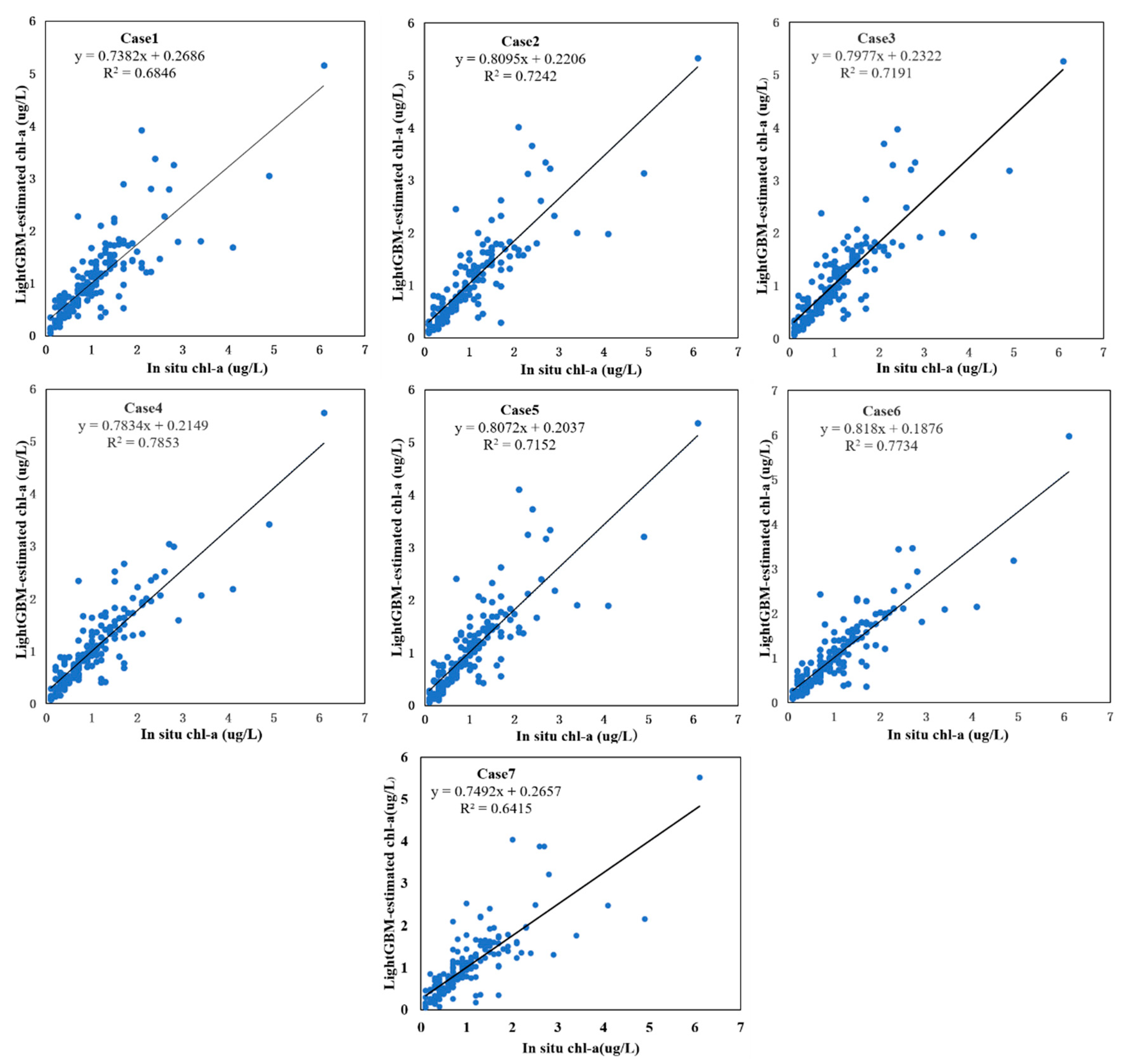
Improving the prediction accuracy is critical for chlorophyll inversion, and this is closely related to the choice of input feature variables. Therefore, on the basis of the LightGBM algorithm, the prediction accuracy of seven feature combinations for each case was evaluated using the testing sets, 181 pairs of OLCI remote sensing reflectance, and in situ chl-a values. The correlations between in situ observed values and predicted values based on the LightGBM model of each case are presented in Figure 3, and the performance indicators calculated for the seven cases are presented in Table 5.
The scatterplots, as shown in Figure 3, indicated that the in situ chl-a values and the LightGBM model predicted values have good correlations for all cases. Particularly, these show a better understanding of chl-a concentration less than 1 ug/L. Through the mutual comparison of all cases, we demonstrated that Case 4 has the best performance, with an RMSE of 0.38 µg/L, MAE of 0.22 µg/L, MAPE of 28.33%, and R2 of 0.785, followed by Case 6, with an RMSE of 0.40 µg/L, MAE of 0.23 µg/L, MAPE of 28.49%, and R2 of 0.773. Here, both Cases 4 and 6 added NFHI as input feature variables. Thus, we believe that NFHI greatly helped improve the prediction accuracy. The main reason is that NFHI used the fluorescence peaks of chl-a, which is in red wavelengths and only carries the chl-a information. It can minimize the influence of TSS and CDOM on the inversion of chl-a concentration. Among all cases, Case 7 has the worst performance, with an RMSE of 0.51 µg/L, MAE of 0.30 µg/L, MAPE of 36.92%, and R2 of 0.641, where only spectral indices were used and without additional spectral bands. This indicates that the model cannot perform well when only considering the spectral indices for the modeling. Among Cases 1 to Cases 6, Case 1 performs worst, with an RMSE of 0.47 µg/L, MAE of 0.27 µg/L, MAPE of 31.42%, and R2 of 0.684, where only ten spectral bands were used and without additional spectral indices. This indicates that the addition of indices is helpful to the accuracy improvement. The prediction accuracies of Cases 2, 3, and 5 are all better than that of Case 1. Cases 2 and 3 have similar results: Case 2 has an RMSE of 0.445 µg/L, MAE of 0.260 µg/L, MAPE of 31.73%, and R2 of 0.724, and Case 3 has an RMSE of 0.447 µg/L, MAE of 0.262 µg/L, MAPE of 31.64%, and R2 of 0.719. Case 2 added the NIR/Red index, whereas Case 3 added NDCI. They both used B11, B9, and B8 in the form of BRs to eliminate uncertainties in the estimation of water remote sensing reflectance in atmospheric correction, seasonal solar azimuth differences, and others. In all the added indices cases, Case 5 has a poor performance, with an RMSE of 0.452 µg/L, MAE of 0.262 µg/L, MAPE of 31.52%, and R2 of 0.715, but it has a better performance than Case 1, indicating that the TBI is also a positive factor for chl-a concentration estimation.
The above clearly demonstrates that the addition of spectral indices, including BRI, NDCI, NFHI, and TBI, can contribute to the improvement of the prediction accuracy of chl-a. These spectral indices are constructed in the form of band combinations using the chl-a sensitive bands to enhance chl-a remote sensing signals. Among these, NFHI is the most beneficial spectral index for improving the chl-a prediction accuracy in the study of Fujian’s coastal waters. However, when all spectral indices added 18 input variables (in Case 6), the result did not demonstrate the best prediction accuracy. In fact, these indices are used solely as factors to establish the regression equation for chl-a predictions. Therefore, although they all have a positive response on chl-a prediction, adding them all for model predictions is still not a good idea. Furthermore, too many dimensions of variables may lead to model instability and complexity. Therefore, the feature variables in Case 4 were eventually chosen for this following study.

4.2. Mapping Chl-a Concentration from the OLCI Images

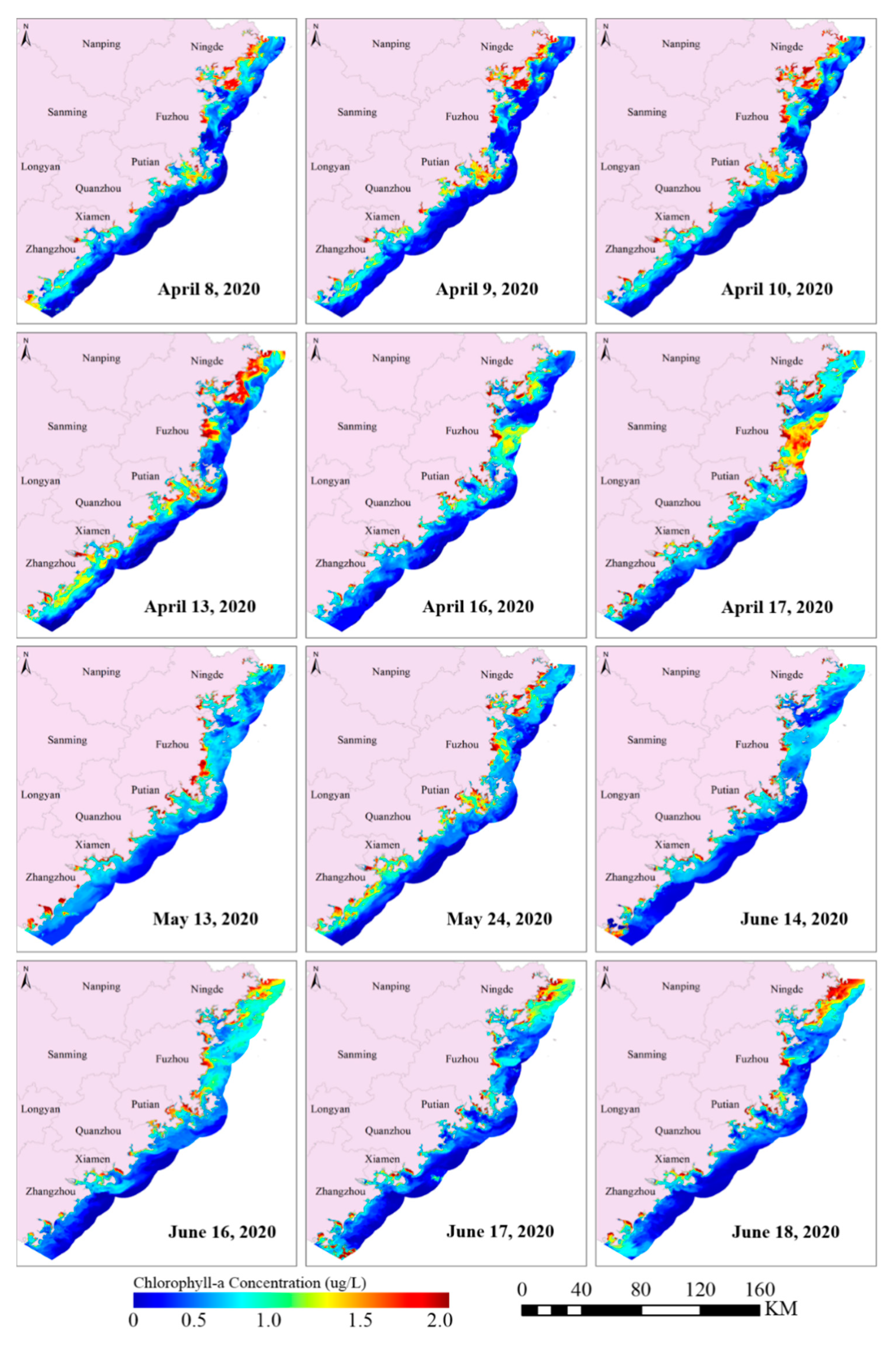
The coastal areas of Fujian are where red tide events seriously occur. Notably, from April to June each year, a high incidence of red tide is observed, according to relevant information released by the Fujian Ocean and Fisheries Bureau (http://hyyyj.fujian.gov.cn/) (accessed on 1 April 2020). Hence, to better understand the temporal and spatial variations of chl-a concentration in Fujian’s coastal waters and evaluate the applicability of the LightGBM-based model to estimate chl-a concentration, we applied the LightGBM model on the OLCI images to map the spatial distribution of chl-a concentration in April to June 2020. In this study, we selected 12 OLCI images (nearly cloudless) of Fujian’s coastal water areas. Then, we used the LightGBM-Case 4 method to obtain the time-series estimation of chl-a concentration in order to track the chl-a concentration variation process. Figure 4 presents the estimated results.
From the results presented in Figure 4, it can be clearly seen that the spatial distribution of chl-a concentration in coastal waters changed daily. From an overall perspective, on 8–10 April 2020, the spatial distributions of chl-a concentration in water were almost similar, and the variation is not evident. The values of chl-a concentration are mainly distributed between 0.5 and 2 ug/L in coastal waters and less than 0.5 ug/L in the open ocean. On 13 April, the chl-a concentration as a whole increased, and the overall spatial pattern was also mostly the same as before. On 16 and 17 April, a significant difference in the variations of chl-a concentration in space was observed. The values of chl-a concentration decreased and were mainly distributed between 0.5 and 1.0 ug/L in most coastal water areas. It should be noted that in the sea near Pingtan Island (Fuzhou), chl-a concentration significantly changed, where the values are mainly greater than 1.0 ug/L, whereas in the previous four phases, the values were less than 0.5 ug/L. The values of chl-a concentration on 17 April were higher than those on 16 April, and the area of variation was also larger. We can also see that in the results for May and June, the temporal and spatial variations of chlorophyll concentration were significant.
With human activity as the main factor causing the change in chl-a concentration, other natural factors also made a common impact, such as the temperature and salinity of the sea water and the changes in the wind direction of ocean currents. According to synoptic data, in mid-April, the coastal weather in Fujian was cloudy to overcast, the water temperature rose, and the wind and waves were relatively small. These conditions are conducive to phytoplankton proliferation and aggregation, and thus, the coastal waters of Fujian entered the peak of the red tide period. Simultaneously, the government focused on this serious issue and conducted encryption monitoring. The field survey results revealed that Thalassiosira subtilis and Skeletonema costatum appeared in the waters in April and May. Our results also provide comprehensive spatial and temporal information as satellite monitoring presents a huge advantage both in time and space for large-scale and real-time monitoring.

4.3. Spatiotemporal Distribution Analysis

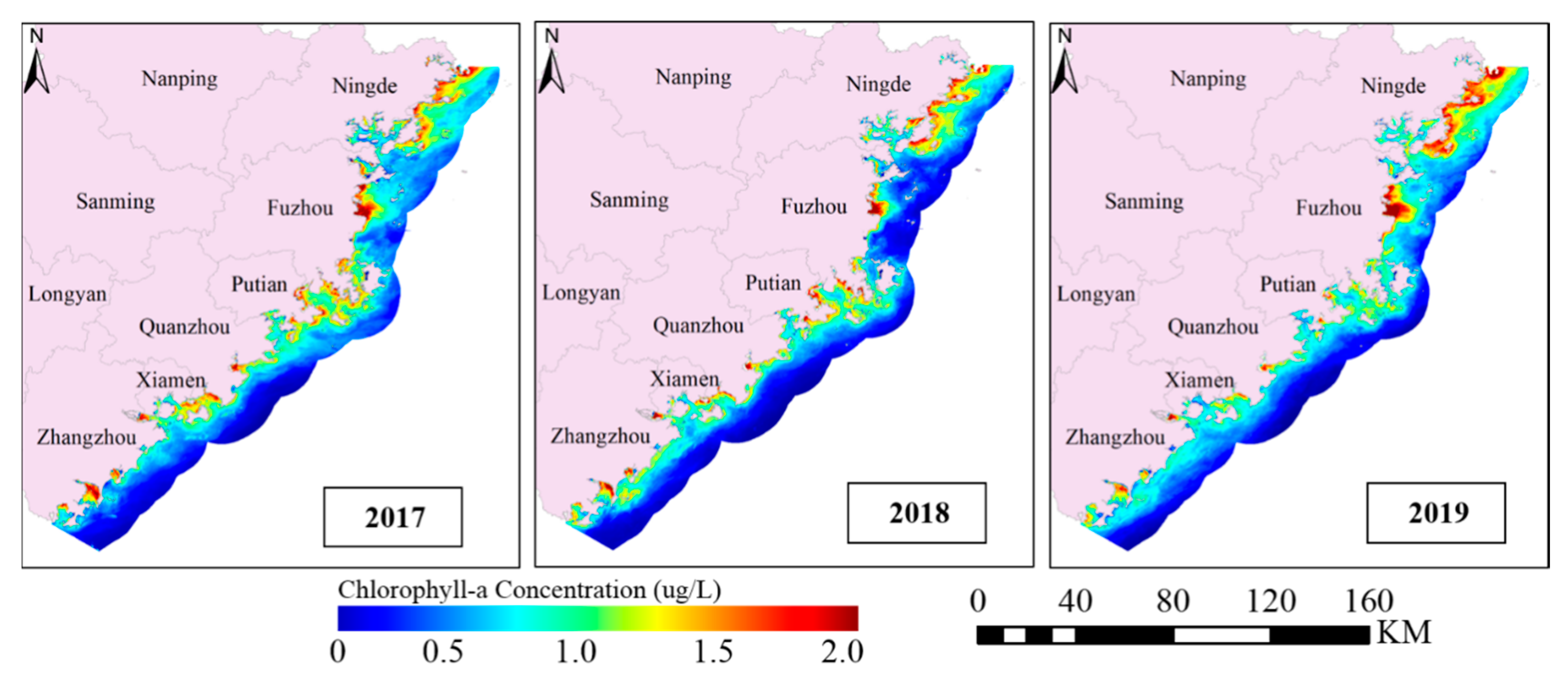
To further understand the characteristics of spatial and temporal distribution in Fujian’s coastal waters, we applied the LightGBM-based model to the OLCI images from 2017 to 2019 to generate time-series chl-a concentration. The annual and monthly averages were calculated on the basis of these time-series chl-a concentration values. Figure 5 and Figure 6 present the spatiotemporal distribution.
Figure 5 presents that, on the whole, the spatial distribution trends of the annual average in 2017–2018 are broadly similar. The values of chl-a concentration are generally higher in the near shore than in the far shore, and the concentration values gradually decrease as the distance from the shoreline increases. This is probably because the internal environment of the coastal waters is complex and changeable and is impacted by human activities (e.g., wastewater discharge, waterway transportation, and aquaculture). Contrarily, in the ocean off the coast, which is almost unaffected by human factors and natural influences, the chl-a concentration values are usually at a low level with small change in the ranges.
Fujian’s coastal water obviously has regional characteristics as it typically hosts case II water. Moreover, the complex and changeable internal environment of the Fujian nearshore region causes distribution differences. The chl-a concentration in the coastal waters is mostly around 1 μg/L but is significantly higher in some bays and river estuaries than in the surrounding open seas. The coastal waters are shallower, and the water bodies are easily disturbed, which results in a nutrient and salt mixture in the whole water layer and thus promotes phytoplankton growth. In addition, there are many harbors in Fujian; this favorable geographical condition promotes aquaculture development. Sansha Bay is one of the most typical aquaculture bays in the coastal areas of China, as shown in Figure 7. The aquaculture activities mainly include cage culture and raft culture. Thus, metabolites and wastewater from farmed bait residues do not easily spread in the bay, resulting in water eutrophication and relatively high chl-a concentration. Another reason is that the coastal area is dense with industrial establishments, thus resulting in a large amount of industrial wastewater carrying terrestrial materials in rivers flowing into the ocean. In the vertical direction, the northern part of Fujian’s coastal waters has a higher chl-a concentration than the other regions. Figure 6 demonstrates that Fujian’s coastal water also has obvious differences in chl-a concentration with time. In spring and summer, the chl-a concentration is higher than in autumn and winter. As the water temperature gradually increases in spring and summer, the water becomes more suitable for phytoplankton growth. Therefore, the chl-a concentration increases to the normal range, and the areas where there are obvious chl-a concentration increases are the bay areas.

4.4. Comparison with Other Previous Algorithms and OLCI L2 Products

To further evaluate the performance of the LightGBM method, we examined the BR algorithm based on NIR/Red and TB algorithm for comparison, which represent the empirical and semiempirical methods in turbid productive coastal waters, respectively, and both have been widely used. Previous studies have demonstrated that the BR algorithm can eliminate the errors caused by different solar altitude angles and observation angles, partially eliminate the interference caused by water surface smoothness and small waves changing with time and space, and counteract some atmospheric effects. Contrarily, the TB algorithm has a definite physical basis and can eliminate some of the effects of suspended sediments. Table 6 presents the two methods based on the OLCI images tested in this study. The specific processes of the methods are as follows: First, x-variable is calculated from OLCI bands; second, the linear regression model is built with the corresponding in situ chl-a data by the least square method; last, the regression models are applied to retrieve chl-a concentration from OLCI images.
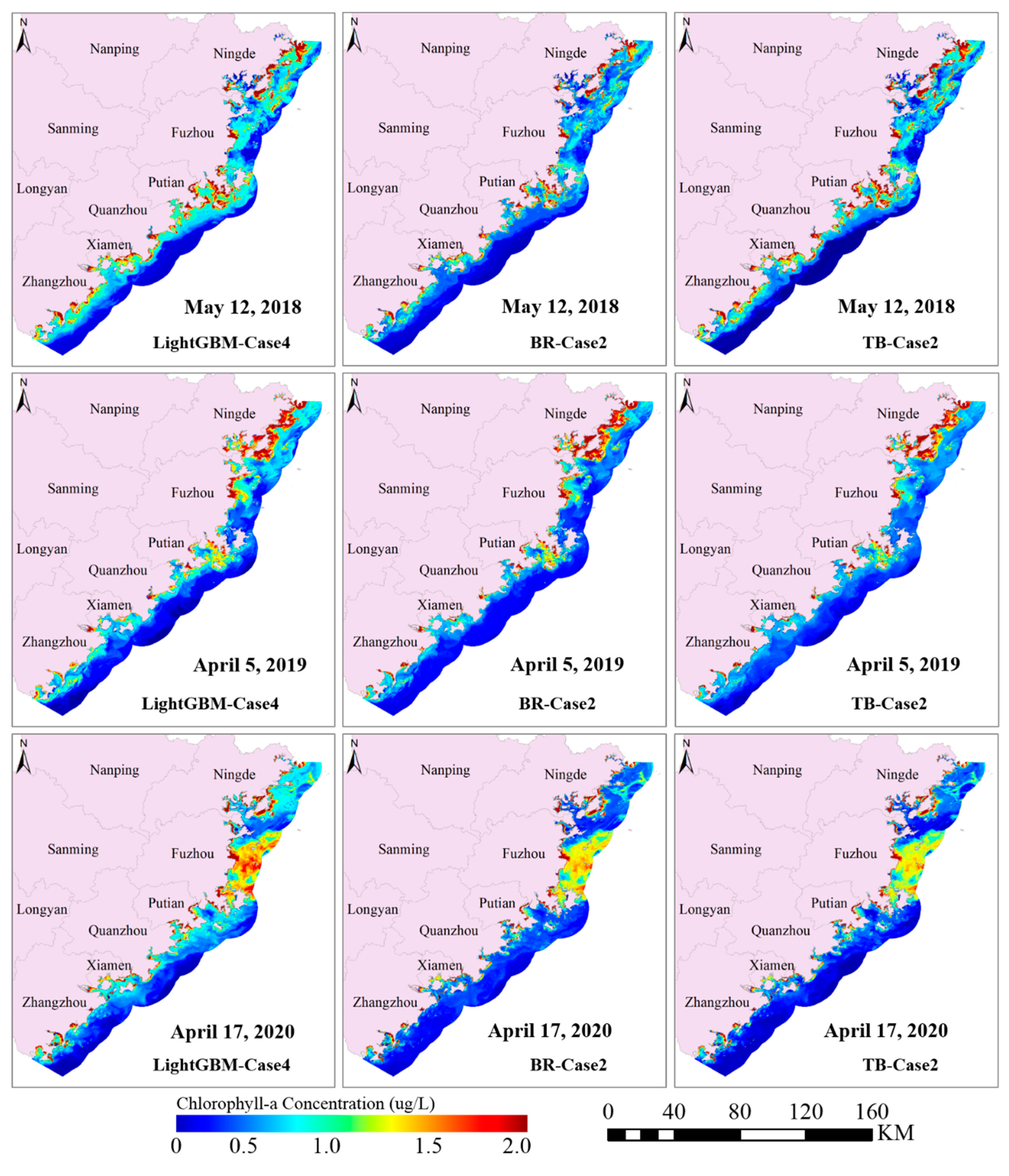
The average RMSE and R2 for the evaluation of the three models are presented in Figure 8. From Figure 8, it can be observed that the LightGBM model has the best accuracy with a lower RMSE and higher R2. Here, we mapped the spatial distribution of chl-a concentration on 12 May 2018, 5 April 2019, and 17 April 2020, in Fujian’s coastal waters based on the LightGBM-Case 4, BR-Case 2, and TB-Case 2 models to further compare the spatial distribution. The results are presented in Figure 9. The results also indicate that the LightGBM-based model has a better applicability considering the space than the traditional methods for the estimation of chl-a concentration in Fujian’s coastal waters.
Figure 9 demonstrates that the spatial distribution patterns of chl-a concentration using BR and TB models are very similar. While the mapping results derived from these two models can also obtain the general spatial distribution pattern of chl-a in Fujian’s coastal waters, such as in areas with higher chl-a concentration, the models are less sensitive to the changes in chl-a in some waters with a lower concentration. Contrarily, the LightGBM-Case 4 model can capture more information about chl-a. This may be because the LightGBM-Case 4 model used the continuous spectral bands B3–B12 (442.5–753.75 nm), which carry the main remote sensing signal of chl-a, like the fluorescence band of chl-a. Contrarily, the BR and TB methods only used two or three bands. Moreover, they only considered the linear relationship between independent and dependent variables, whereas the optical properties of case II water bodies are complex, and the relationship between the concentration of chl-a and the spectrum cannot be completely expressed linearly. As a machine learning method, the LightGBM-Case 4 model can deal with any nonlinear relationship. Moreover, the LightGBM-Case 4 model inputs more spectral features than the BR and TB methods. In addition to the performance differences in the models themselves, the limited number of samples and the accuracy of the atmospheric correction algorithm affect the prediction accuracy of the model to some extent. Moreover, natural and human activities as well as other factors, such as meteorological, hydrological, and aquacultural factors, influence chl-a concentration. More influencing factors should be comprehensively considered to render the remote sensing monitoring model more reliable.
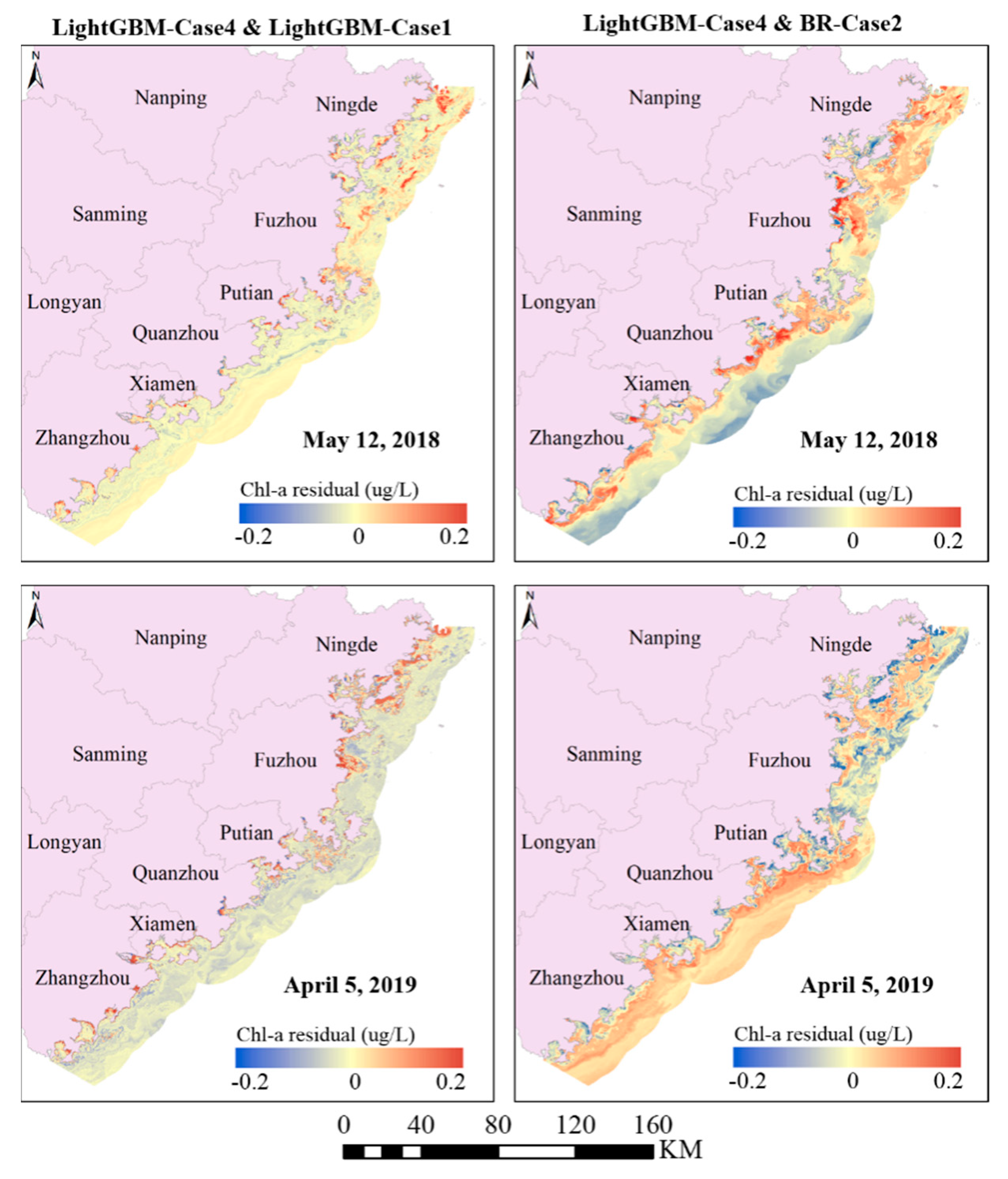
In order to show the result difference more intuitively between different models, we mapped the estimated chl-a bias between LightGBM-Case 4 and LightGBM-Case 1, and LightGBM-Case 4 and BR-Case 2. Figure 10 showed that the bias between the two LightGBM models (Case 4 and Case 1) are very small. While for the two different methods (LightGBM and BR), the bias is much greater. This indicated that the performance difference between LightGBM and BR models is relatively significant.
Ocean color missions are of great significance for the marine environment monitoring. It is important to compare the LightGBM-estimated chl-a concentration with the existing ocean color products. Here, we employed two kinds of OLCI L2 chl-a concentration products for comparison and validation; one is OC4Me chl-a concentration products (based on the OC4Me algorithm) [6], the other is NN chl-a concentration products (based on the Inverse Modelling Technique (IMT) Neural Net algorithm).
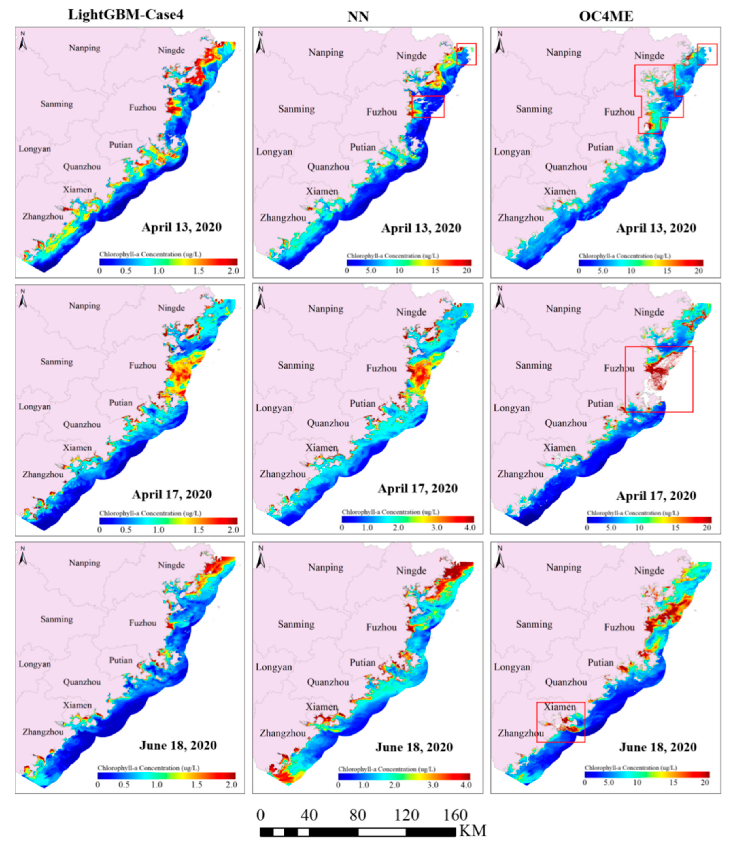
Figure 11 presented the spatial distribution of chl-a concentration based on the LightGBM-Case 4 model, NN algorithm, and OC4ME algorithm. In general, chl-a concentration values based on NN and OC4ME algorithms are significantly higher than LightGBM-Case 4 estimated values; especially OC4ME estimated values, which were overestimated to 20 ug/L. In fact, the values of chl-a concentration are mainly distributed between 0 and 2 ug/L in the coastal waters according to in situ measurement. The spatial distribution of chl-a concentration for the LightGBM model and NN algorithm are generally consistent. However, the OLCI L2 products are not spatially complete, especially the OC4ME products. Figure 11 presented that there are some missing values for chl-a concentration based on the NN algorithm and OC4ME algorithm (shown in the red polygon), while the LightGBM-estimated result is spatially complete. Overall, the LightGBM-estimated product for Fujian’s coastal waters has higher quality than existing OLCI L2 products.

5. Discussion

At present, OLCI is a good option for quickly mapping and retrieving water quality parameter information over large-scale coastal waters due to the high spectral resolution and temporal resolution. With the ocean observation mission of Sentinel-3A and Sentinel-3B satellites, the OLCI data can be obtained almost daily. However, the imaging quality is always subject to the weather, especially in the cloudy and rainy subtropical areas like Fujian. This reduces the usability of the OLCI images for ocean color study, but this meteorological factor is inevitable for optical remote sensing. In the future, we should consider the fusion of multi-source satellite data to obtain more ocean color information. Moreover, the atmospheric correction is significant for ocean color retrieval. The atmospheric correction quality has great influence on the inversion result from remote sensing. A suitable atmospheric correction method can guarantee high-quality reflectance data for ocean color modeling.
Although ocean color missions have provided us abundant ocean color products, their applicability for local areas has not been verified. In this study, we compared the LightGBM-based chl-a product with another two OLCI L2 products (based on NN and OC4ME algorithms). Although the spatial distribution of chl-a concentration from these three methods are generally similar, the ranges of chl-a values from each method are quite different. The main reason is that the in situ data for NN and OC4ME modeling is measured from various ocean regions over the past decades, while in situ data for LightGBM modeling is collected from the coastal waters of Fujian. Thus, the OLCI L2 products are not well suitable for ocean color study in Fujian’s coastal waters. Thus far, there has been still many challenges in developing a universal inversion model for chl-a concentration estimation of global waters due to the significant differences in the optical properties of water bodies over different regions. Although the LightGBM method has yielded good results in the coastal waters of Fujian, the spatial applicability is still the limitation of this approach. However, our method itself has important reference value for the ocean color study in other coastal areas.

6. Conclusions

This study aimed to establish a robust and efficient model based on an advanced machine learning method to estimate chl-a concentration from a new-generation OLCI instrument in coastal waters with complex optical properties. In this study, we proposed a novel gradient boosting method, known as LightGBM, to retrieve the chl-a concentration by combining multitemporal OLCI data with in situ data in Fujian’s coastal waters. The performance of the model was quantitatively evaluated using statistical indicators RMSE, MAE, MAPE, and R2. The study demonstrated that the accuracy of the LightGBM model was higher than that of the BR algorithm, indicating that LightGBM is better suited for chl-a estimation in Fujian’s coastal waters. Moreover, we validated the applicability of the LightGBM-based model for chl-a concentration estimation and analyzed the spatiotemporal distribution of Fujian’s coastal waters.
The inputs of feature variables are important for LightGBM-based chl-a concentration estimation. In this study, we tested four spectral indices (BRI, NDCI, NFHI, and TBI) to evaluate their impact on model performance compared with the spectral band-based model. The results demonstrated that the addition of NFHI indices significantly improved the prediction accuracy, with an RMSE of 0.38 µg/L, MAE of 0.22 µg/L, MAPE of 28.33%, and R2 of 0.77. One advantage of machine learning methods (e.g., LightGBM) is that they can handle multidimensional variables, and the feature variables greatly impact the machine learning performance. Thus, it is important to construct more meaningful additional features based on the initial spectral features to improve the prediction performance. In future studies, we would like to determine more useful spectral indices as input features to enhance the chl-a signal from satellite remote sensing reflectance to further improve the accuracy of the LightGBM model. This would require a deeper understanding of the complex optical properties of Fujian’s coastal waters.
The quality of data sets largely limit the performance of models based on machine learning. One is the quality of satellite remote sensing data (spectral resolution, spatial resolution, temporal resolution, and signal-to-noise ratio). Moreover, to further improve the data collected from float stations, improved uniformity and adequacy for the float spatial distribution are required. Meanwhile, except for optical parameters from satellite data directly related to chlorophyll concentration, other environmental factors (including temperature, light, nutrients, microelements, and rainfall) that may influence chl-a concentration would be considered in future studies.

Author Contributions

Conceptualization, H.S.; methodology, X.L.; validation, X.L. and W.W.; formal analysis, H.S. and X.L.; investigation, Z.C.; data curation, X.L. and W.L.; writing—original draft preparation, H.S. and X.L.; writing—review and editing, H.S. and H.Z.; visualization, X.L.; supervision, H.S. and H.Z.; funding acquisition, H.S. All authors have read and agreed to the published version of the manuscript.

Funding

This research was funded by National Natural Science Foundation of China (grant number: 41971384, 41630963, 41906019), the Strategic Priority Research Program of the Chinese Academy of Sciences, CASEarth (XDA19080103), Open Funding of Guangdong Key Laboratory of Ocean Remote Sensing (2017B030301005-LORS2004), and Natural Science Foundation of Fujian Province (2019J01650).

Institutional Review Board Statement

Not applicable.

Informed Consent Statement

Not applicable.

Data Availability Statement

The data presented in this study are available on request from the corresponding author.

Acknowledgments

We thank the European Space Agency (ESA) data hub for the Sentinel-3 OLCI data (https://scihub.copernicus.eu/) and Fujian Marine Forecasts for the in situ data (http://www.fjhyyb.cn/Ocean863Web_MAIN/), which are freely accessible to the public.

Conflicts of Interest

The authors declare no conflict of interest.

References

  1. Harvey, E.T.; Kratzer, S.; Philipson, P. Satellite-based water quality monitoring for improved spatial and temporal retrieval of chlorophyll-a in coastal waters. Remote Sens. Environ. 2015, 158, 417–430. [Google Scholar] [CrossRef]
  2. Blix, K.; Li, J.; Massicotte, P.; Matsuoka, A. Developing a New Machine-Learning Algorithm for Estimating Chlorophyll-a Concentration in Optically Complex Waters: A Case Study for High Northern Latitude Waters by Using Sentinel 3 OLCI. Remote Sens. 2019, 11, 2076. [Google Scholar] [CrossRef] [Green Version]
  3. Harding, L.W., Jr.; Mallonee, M.E.; Perry, E.S. Toward a Predictive Understanding of Primary Productivity in a Temperate, Partially Stratified Estuary. Estuar. Coast. Shelf Sci. 2002, 55, 437–463. [Google Scholar] [CrossRef]
  4. Moses, W.J.; Gitelson, A.A.; Berdnikov, S.; Povazhnyy, V. Estimation of chlorophyll- a concentration in case II waters using MODIS and MERIS data—successes and challenges. Environ. Res. Lett. 2009, 4, 045005. [Google Scholar] [CrossRef] [Green Version]
  5. Hafeez, S.; Wong, M.S.; Ho, H.C.; Nazeer, M.; Nichol, J.E.; Abbas, S.; Tang, D.; Lee, K.-H.; Pun, L. Comparison of Machine Learning Algorithms for Retrieval of Water Quality Indicators in Case-II Waters: A Case Study of Hong Kong. Remote Sens. 2019, 11, 617. [Google Scholar] [CrossRef] [Green Version]
  6. O’Reilly, J.E.; Werdell, P.J. Chlorophyll algorithms for ocean color sensors—OC4, OC5 & OC6. Remote Sens. Environ. 2019, 229, 32–47. [Google Scholar] [CrossRef] [PubMed]
  7. Gordon, H.R.; Clark, D.K.; Brown, J.W.; Brown, O.B.; Evans, R.H.; Broenkow, W.W. Phytoplankton pigment concentrations in the Middle Atlantic Bight: Comparison of ship determinations and CZCS estimates. Appl. Opt. 1983, 22, 20–36. [Google Scholar] [CrossRef]
  8. George, D.G.; Malthus, T.J. Using a compact airborne spectrographic imager to monitor phytoplankton biomass in a series of lakes in north Wales. Sci. Total Environ. 2001, 268, 215–226. [Google Scholar] [CrossRef]
  9. Zhang, F.; Li, J.; Shen, Q.; Zhang, B.; Tian, L.; Ye, H.; Wang, S.; Lu, Z. A soft-classification-based chlorophyll-a estimation method using MERIS data in the highly turbid and eutrophic Taihu Lake. Int. J. Appl. Earth Obs. Geoinf. 2019, 74, 138–149. [Google Scholar] [CrossRef]
  10. Yang, Z.; Reiter, M.; Munyei, N. Estimation of chlorophyll-a concentrations in diverse water bodies using ratio-based NIR/Red indices. Remote Sens. Appl. Soc. Environ. 2017, 6, 52–58. [Google Scholar] [CrossRef]
  11. Tao, B.; Mao, Z.; Pan, D.; Shen, Y.; Zhu, Q.; Chen, J. Influence of bio-optical parameter variability on the reflectance peak position in the red band of algal bloom waters. Ecol. Inform. 2013, 16, 17–24. [Google Scholar] [CrossRef]
  12. Watanabe, F.S.Y.; Alcântara, E.; Stech, J.L. High performance of chlorophyll- a prediction algorithms based on simulated OLCI Sentinel-3A bands in cyanobacteria-dominated inland waters. Adv. Space Res. 2018, 62, 265–273. [Google Scholar] [CrossRef] [Green Version]
  13. Mishra, S.; Mishra, D.R. Normalized difference chlorophyll index: A novel model for remote estimation of chlorophyll-a concentration in turbid productive waters. Remote Sens. Environ. 2012, 117, 394–406. [Google Scholar] [CrossRef]
  14. Gower, J.F.R.; Doerffer, R.; Borstad, G.A. Interpretation of the 685nm peak in water-leaving radiance spectra in terms of fluorescence, absorption and scattering, and its observation by MERIS. Int. J. Remote Sens. 2010, 20, 1771–1786. [Google Scholar] [CrossRef]
  15. El-Habashi, A.; Ioannou, I.; Tomlinson, M.C.; Stumpf, R.P.; Ahmed, S. Satellite Retrievals of Karenia brevis Harmful Algal Blooms in the West Florida Shelf Using Neural Networks and Comparisons with Other Techniques. Remote Sens. 2016, 8, 377. [Google Scholar] [CrossRef] [Green Version]
  16. Molkov, А.А.; Fedorov, S.V.; Pelevin, V.V.; Korchemkina, E.N. Regional Models for High-Resolution Retrieval of Chlorophyll a and TSM Concentrations in the Gorky Reservoir by Sentinel-2 Imagery. Remote Sens. 2019, 11, 1215. [Google Scholar] [CrossRef] [Green Version]
  17. Binding, C.E.; Greenberg, T.A.; Bukata, R.P. Time series analysis of algal blooms in Lake of the Woods using the MERIS maximum chlorophyll index. J. Plankton Res. 2011, 33, 1847–1852. [Google Scholar] [CrossRef] [Green Version]
  18. Hu, C. A novel ocean color index to detect floating algae in the global oceans. Remote Sens. Environ. 2009, 113, 2118–2129. [Google Scholar] [CrossRef]
  19. Chen, X.; Shang, S.; Lee, Z.; Qi, L.; Yan, J.; Li, Y. High-frequency observation of floating algae from AHI on Himawari-8. Remote Sens. Environ. 2019, 227, 151–161. [Google Scholar] [CrossRef]
  20. Garcia, R.A.; Fearns, P.; Keesing, J.K.; Liu, D. Quantification of floating macroalgae blooms using the scaled algae index. J. Geophys. Res. Oceans 2013, 118, 26–42. [Google Scholar] [CrossRef] [Green Version]
  21. Odermatt, D.; Gitelson, A.; Brando, E. Review of constituent retrieval in optically deep and complex waters from satellite imagery. Remote Sens. Environ. 2012, 118, 116–126. [Google Scholar] [CrossRef] [Green Version]
  22. Gitelson, A.A.; Dall’Olmo, G.; Moses, W.; Rundquist, D.; Barrow, T.; Fisher, T.R.; Gurlin, D.; Holz, J. A simple semi-analytical model for remote estimation of chlorophyll-a in turbid waters: Validation. Remote Sens. Environ. 2008, 112, 3582–3593. [Google Scholar] [CrossRef]
  23. Hu, C.; Lee, Z.; Bryan, F. Chlorophyll-a Algorithms for Oligotrophic Oceans: A Novel Approach Based on Three-Band Reflectance Difference. J. Geophys. Res. Atmos. 2012, 117, 92–99. [Google Scholar] [CrossRef] [Green Version]
  24. Huang, C.; Zou, J.; Li, Y.; Yang, H.; Shi, K.; Li, J.; Wang, Y.; Chena, X.; Zheng, F. Assessment of NIR-red algorithms for observation of chlorophyll-a in highly turbid inland waters in China. ISPRS J. Photogramm. Remote Sens. 2014, 93, 29–39. [Google Scholar] [CrossRef]
  25. Sun, D.; Hu, C.; Qiu, Z.; Cannizzaro, J.P.; Barnes, B.B. Influence of a red band-based water classification approach on chlorophyll algorithms for optically complex estuaries. Remote Sens. Environ. 2004, 155, 289–302. [Google Scholar] [CrossRef]
  26. Le, C.; Li, Y.; Zha, Y.; Sun, D.; Huang, C.; Lu, H. A four-band semi-analytical model for estimating chlorophyll a in highly turbid lakes: The case of Taihu Lake, China. Remote Sens. Environ. 2009, 113, 1175–1182. [Google Scholar] [CrossRef]
  27. Pahlevan, N.; Smith, B.; Schalles, J.; Binding, C.; Cao, Z.; Ma, R.; Alikas, K.; Kangro, K.; Gurlin, D.; Hà, N.; et al. Seamless retrievals of chlorophyll-a from Sentinel-2 (MSI) and Sentinel-3 (OLCI) in inland and coastal waters: A machine-learning approach. Remote Sens. Environ. 2020, 240, 111604. [Google Scholar] [CrossRef]
  28. Charantonis, A.; Badran, F.; Thiria, S. Retrieving the evolution of vertical profiles of Chlorophyll-a from satellite observations using Hidden Markov Models and Self-Organizing Topological Maps. Remote Sens. Environ. 2015, 163, 229–239. [Google Scholar] [CrossRef]
  29. Ruescas, A.; Hieronymi, M.; Mateo-Garcia, G.; Koponen, S.; Kallio, K.; Camps-Valls, G. Machine Learning Regression Approaches for Colored Dissolved Organic Matter (CDOM) Retrieval with S2-MSI and S3-OLCI Simulated Data. Remote Sens. 2018, 10, 786. [Google Scholar] [CrossRef] [Green Version]
  30. Blix, K.; Pálffy, K.; Tóth, V.R.; Eltoft, T. Remote Sensing of Water Quality Parameters over Lake Balaton by Using Sentinel-3 OLCI. Water 2018, 10, 1428. [Google Scholar] [CrossRef] [Green Version]
  31. Lei, S.; Xu, J.; Li, Y.; Du, C.; Liu, G.; Zheng, Z.; Xu, Y.; Lyu, H.; Mu, M.; Miao, S.; et al. An approach for retrieval of horizontal and vertical distribution of total suspended matter concentration from GOCI data over Lake Hongze. Sci. Total Environ. 2020, 700, 134524. [Google Scholar] [CrossRef]
  32. Zhang, Y.; Pulliainen, J.; Koponen, S.; Hallikainen, M. Application of an empirical neural network to surface water quality estimation in the Gulf of Finland using combined optical data and microwave data. Remote Sens. Environ. 2002, 81, 327–336. [Google Scholar] [CrossRef]
  33. Kim, Y.-H.; Im, J.; Ha, H.K.; Choi, J.-K.; Ha, S. Machine learning approaches to coastal water quality monitoring using GOCI satellite data. GIScience Remote Sens. 2014, 51, 158–174. [Google Scholar] [CrossRef]
  34. Kong, X.; Sun, Y.; Su, R.; Shi, X. Real-time eutrophication status evaluation of coastal waters using support vector machine with grid search algorithm. Mar. Pollut. Bull. 2017, 119, 307–319. [Google Scholar] [CrossRef] [PubMed]
  35. Huang, G.; Wu, L.; Ma, X.; Zhang, W.; Fan, J.; Yu, X.; Zeng, W.; Zhou, H. Evaluation of CatBoost method for prediction of reference evapotranspiration in humid regions. J. Hydrol. 2019, 574, 1029–1041. [Google Scholar] [CrossRef]
  36. Su, H.; Yang, X.; Lu, W.; Yan, X.-H. Estimating Subsurface Thermohaline Structure of the Global Ocean Using Surface Remote Sensing Observations. Remote Sens. 2019, 11, 1598. [Google Scholar] [CrossRef] [Green Version]
  37. Mouw, B.; Greb, S.; Aurin, D. Aquatic color radiometry remote sensing of coastal and inland waters: Challenges and recom-mendations for future satellite missions. Remote Sens. Environ. 2015, 160, 15–30. [Google Scholar] [CrossRef]
  38. Nazeer, M.; Nichol, J.E. Development and application of a remote sensing-based Chlorophyll-a concentration prediction model for complex coastal waters of Hong Kong. J. Hydrol. 2016, 532, 80–89. [Google Scholar] [CrossRef]
  39. Bernardo, N.; Watanabe, F.; Rodrigues, T.; Alcântara, E. Evaluation of the suitability of MODIS, OLCI and OLI for mapping the distribution of total suspended matter in the Barra Bonita Reservoir (Tietê River, Brazil). Remote Sens. Appl. Soc. Environ. 2016, 4, 68–82. [Google Scholar] [CrossRef]
  40. Fu, Y.; Xu, S.; Zhang, C.; Sun, Y. Spatial downscaling of MODIS Chlorophyll-a using Landsat 8 images for complex coastal water monitoring. Estuar. Coast. Shelf Sci. 2018, 209, 149–159. [Google Scholar] [CrossRef]
  41. Brockmann, C.; Doerffer, R.; Peters, M.; Kerstin, S.; Embacher, S.; Ruescas, A. Evolution of the C2RCC neural network for sentinel 2 and 3 for the retrieval of ocean colour products in normal and extreme optically complex waters. ESASP 2016, 740, 54. [Google Scholar]
  42. Toming, K.; Kutser, T.; Uiboupin, R.; Arikas, A.; Vahter, K.; Paavel, B. Mapping Water Quality Parameters with Sentinel-3 Ocean and Land Colour Instrument imagery in the Baltic Sea. Remote Sens. 2017, 9, 1070. [Google Scholar] [CrossRef] [Green Version]
  43. Kyryliuk, D.; Kratzer, S. Evaluation of Sentinel-3A OLCI Products Derived Using the Case-2 Regional CoastColour Processor over the Baltic Sea. Sensors 2019, 19, 3609. [Google Scholar] [CrossRef] [PubMed] [Green Version]
  44. Friedman, J.H. Greedy function approximation: A gradient boosting machine. Ann. Stat. 2001, 29, 1189–1232. [Google Scholar] [CrossRef]
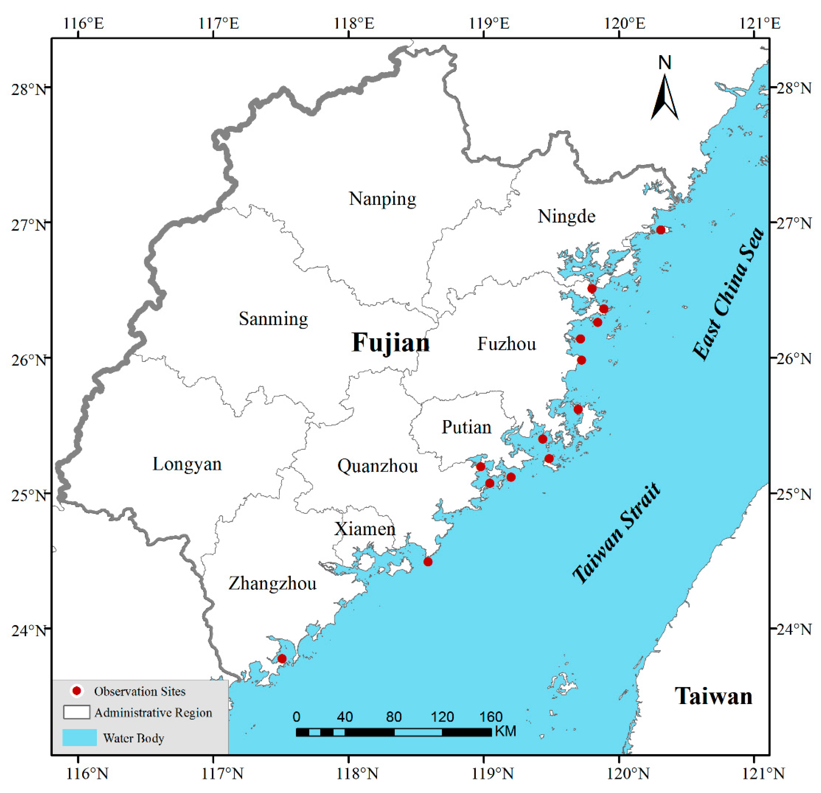
Figure 1. The location of Fujian (China) and the spatial distribution of in situ observation stations in Fujian’s coastal waters.
Remotesensing 13 00576 g001
Figure 2. The relationship between regression error and n_estimators in the Light Gradient Boosting Machine (LightGBM) model.
Remotesensing 13 00576 g002
Figure 3. Scatter plots between the LightGBM model-estimated and in situ ch1-a concentration.
Remotesensing 13 00576 g003
Figure 4. The estimated chl-a concentration and variation using the LightGBM-Case 4 model from the OLCI images of Fujian’s coastal waters in April to June 2020.
Remotesensing 13 00576 g004
Figure 5. Spatial distribution of the annual average chl-a concentration based on the LightGBM-Case 4 model using the OLCI images from 2017 to 2019 in Fujian’s coastal waters.
Remotesensing 13 00576 g005
Figure 6. Spatial distribution of monthly average chl-a concentration based on the LightGBM model using the OLCI images from 2017 to 2019 in Fujian’s coastal waters.
Remotesensing 13 00576 g006
Figure 7. Spatial distribution of chl-a concentration based on the LightGBM model in Sansha Bay of Fujian Province.
Remotesensing 13 00576 g007
Figure 8. The average root-mean-square error (RMSE) and R2 of chl-a concentration estimated using the LightGBM, blue-green band ratio (BR), and three-band (TB) models.
Remotesensing 13 00576 g008
Figure 9. Spatial distribution of chl-a concentration based on the LightGBM-Case 4, BR-Case 2, and TB-Case 2 using the OLCI images on 12 May 2018, 5 April 2019, and 17 April 2020, in Fujian’s coastal waters.
Remotesensing 13 00576 g009
Figure 10. Spatial distribution of estimated chl-a concentration bias between different models. The left column is the bias between LightGBM-Case 4 and LightGBM-Case 1 models, the right column is the bias between LightGBM-Case 4 and BR-Case 2 models.
Remotesensing 13 00576 g010
Figure 11. Spatial distribution of chl-a concentration based on the LightGBM-Case 4 using the OLCI images (left column) and OLCI L2 chl-a products based on the NN algorithm (middle column), and OC4ME algorithm (right column) on 13 April 2020, 17 April 2020, and 18 June 2020 in Fujian’s coastal waters.
Remotesensing 13 00576 g011
Table 1. Summary of the S3 Ocean and Land Color Instrument (OLCI) spectral bands used in this study.
Band NumberCentral Wavelength (nm)Bandwidth (nm)Signal-to-Noise Ratio
Band 3442.5101811
Band 4490101541
Band 5510101488
Band 6560101280
Band 762010997
Band 866510883
Band 9673.757.5707
Band 10681.257.5745
Band 11708.7510785
Band 12753.757.5605
Table 2. Description of the input variables from OLCI.
Feature VariablesThe Full NameExpression FormsReference
Spectral bandsSpectral bandsB3, B4, B5, B6, B7, B8, B9, B10, B11, B12[27]
BRIBand ratio indexB11/B8[10]
B11/B9
NDCINormalized difference chlorophyll index(B11 − B8)/(B11 + B8)[13]
(B11 − B9)/(B11 + B9)
NFHINormalized fluorescence height indexB10/B6[15]
B10/B9
TBIThree-band index(1/B8 − 1/B11) × B12[22]
(1/B9 − 1/B11) × B12
Table 3. Information on the experimental cases.
ExperimentInput Features
Case 1Spectral bands
Case 2Spectral bands + BRI
Case 3Spectral bands + NDCI
Case 4Spectral bands + NFHI
Case 5Spectral bands + TBI
Case 6All variables
Case 7Spectral indices
Table 4. The description of the imperative parameters of the LightGBM model and the optimal values after tuning.
ParametersMeaning (Default Values)RangesOptimal Values
learning_rateShrinkage rate (0.1)[0, 1]0.05
n_estimatorsThe number of trees (100)[1, ∝]400
num_leavesMax number of leaves in one tree (31)[1, 131072]40
lambda_L1L2 regularization (0)[0, ∝]1
lambda_L2L1 regularization (0)[0, ∝]3
boosting_typeBoosting type (gbdt)gbdt, rf, dart, gossgbdt
Table 5. Performance metrics associated with the LightGBM model-estimated ch1-a concentration.
Experimental CasesRMSEMAEMAPE (%)R2
Case 10.4690.27431.420.685
Case 20.4450.26031.730.724
Case 30.4470.26231.640.719
Case 40.3880.22528.330.785
Case 50.4520.26231.520.715
Case 60.3970.22528.490.772
Case 70.5090.30436.920.641
Table 6. List of the representatives of the empirical and semiempirical methods tested in this study.
ModelExpressionx-VariableRMSER2
BR-Case 1y = 4.2969x − 1.8276Rrs (708.75)/Rrs (665)0.6350.586
BR-Case 2y = 3.6923x − 1.6779Rrs (708.75)/Rrs (673.75)0.6340.588
TB-Case 1y = 15.416x + 2.426(Rrs (665) −1 − Rrs (681.25) −1) × Rrs (753.75)0.7190.586
TB-Case 2y = 12.952x + 1.956(Rrs (673.75) −1 − Rrs (681.25) −1) × Rrs (753.75)0.6360.587
Publisher’s Note: MDPI stays neutral with regard to jurisdictional claims in published maps and institutional affiliations.