
Multiscaling NDVI Series Analysis of Rainfed Cereal in Central Spain

 ,
, 
Abstract
1. Introduction
2. Materials and Methods
2.1. Site Description and Zones Selection
2.2. Soil and Weather
2.3. Earth Observation Data
2.4. Plots and Pixels Selection Criteria
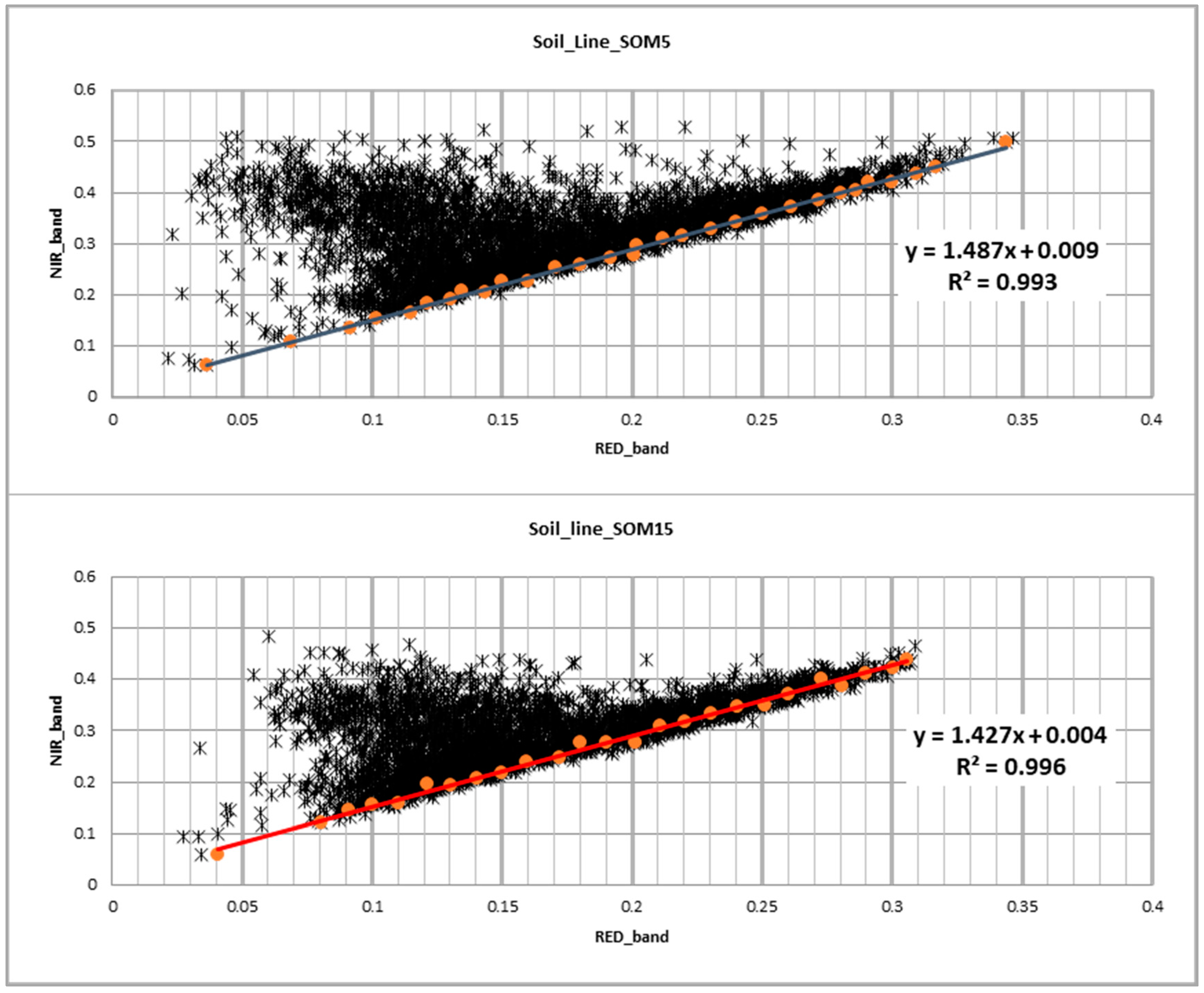
2.5. Soils Reflectance Characteristics
2.6. NDVI Series and Statistics
2.7. Generalised Structure Function (GSF)
3. Results
3.1. Soils Reflectance Statistics
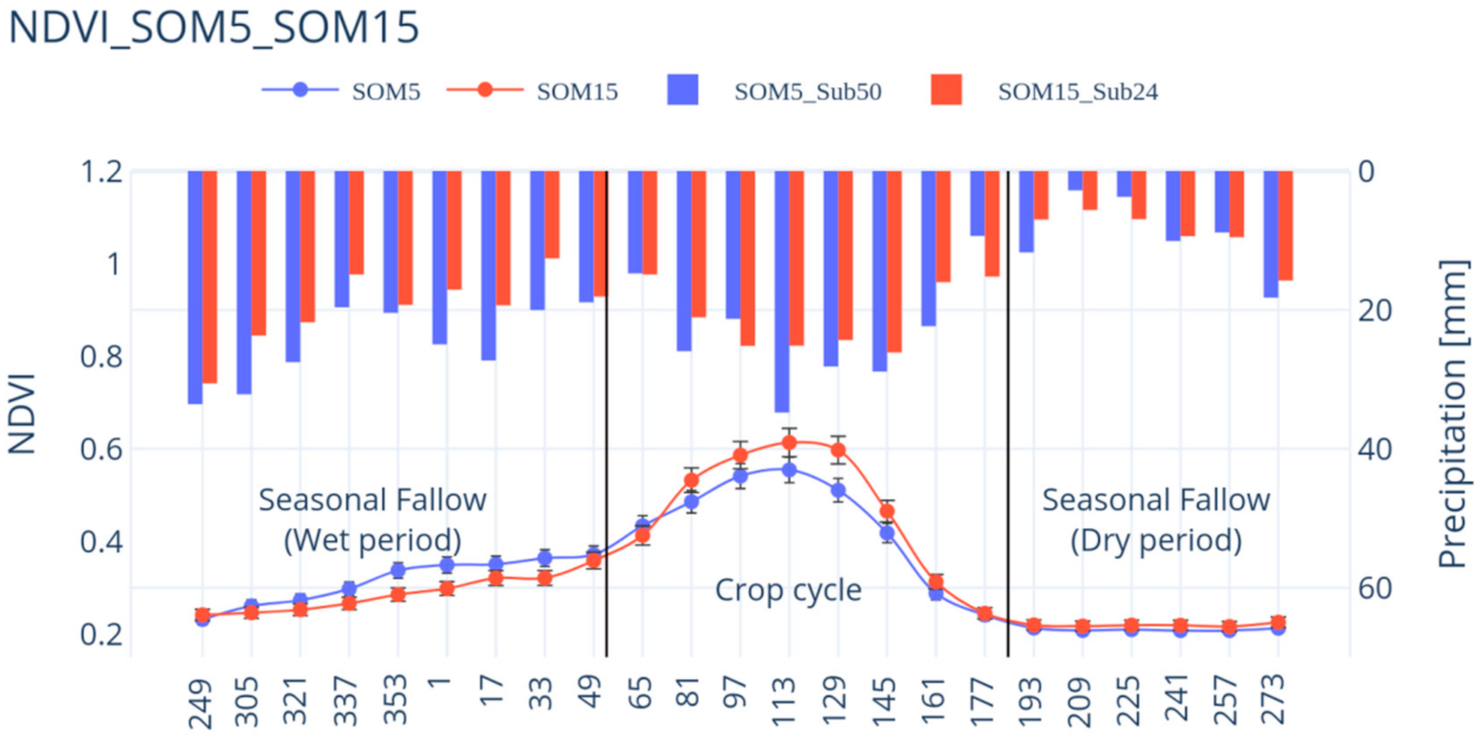
3.2. NDVI Statistics
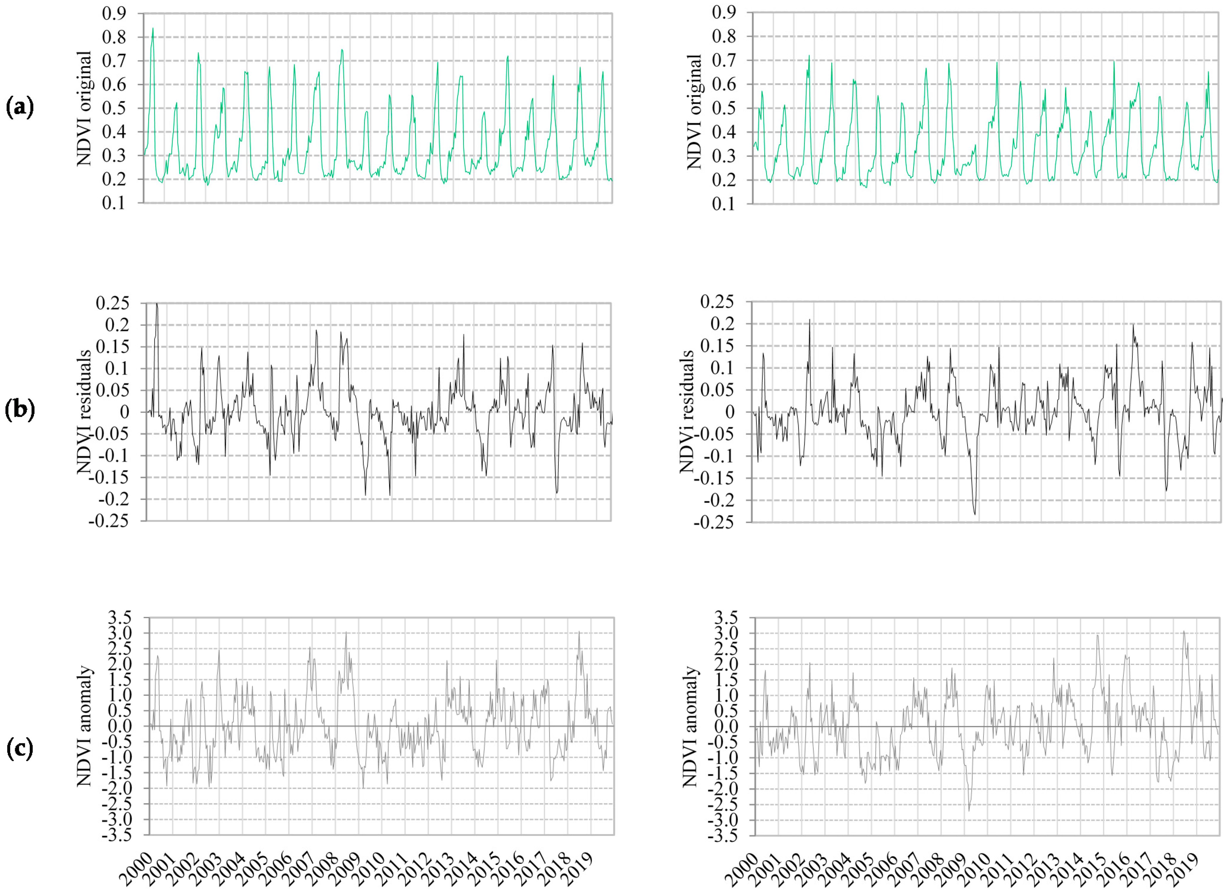
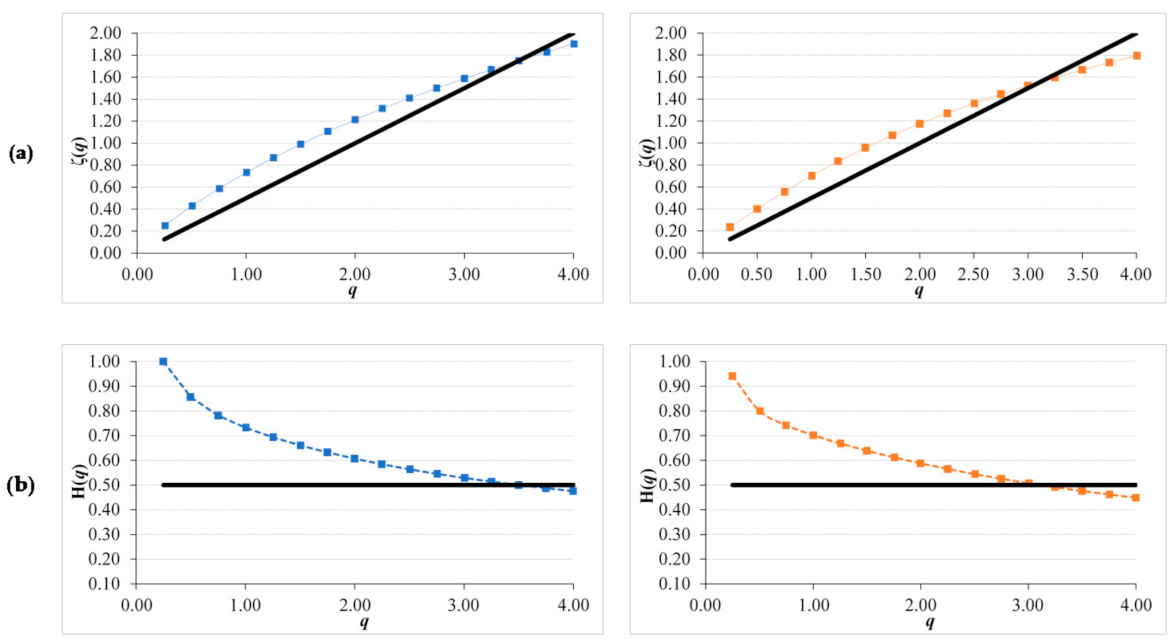
3.3. Scaling Characteristics of NDVI Original Series
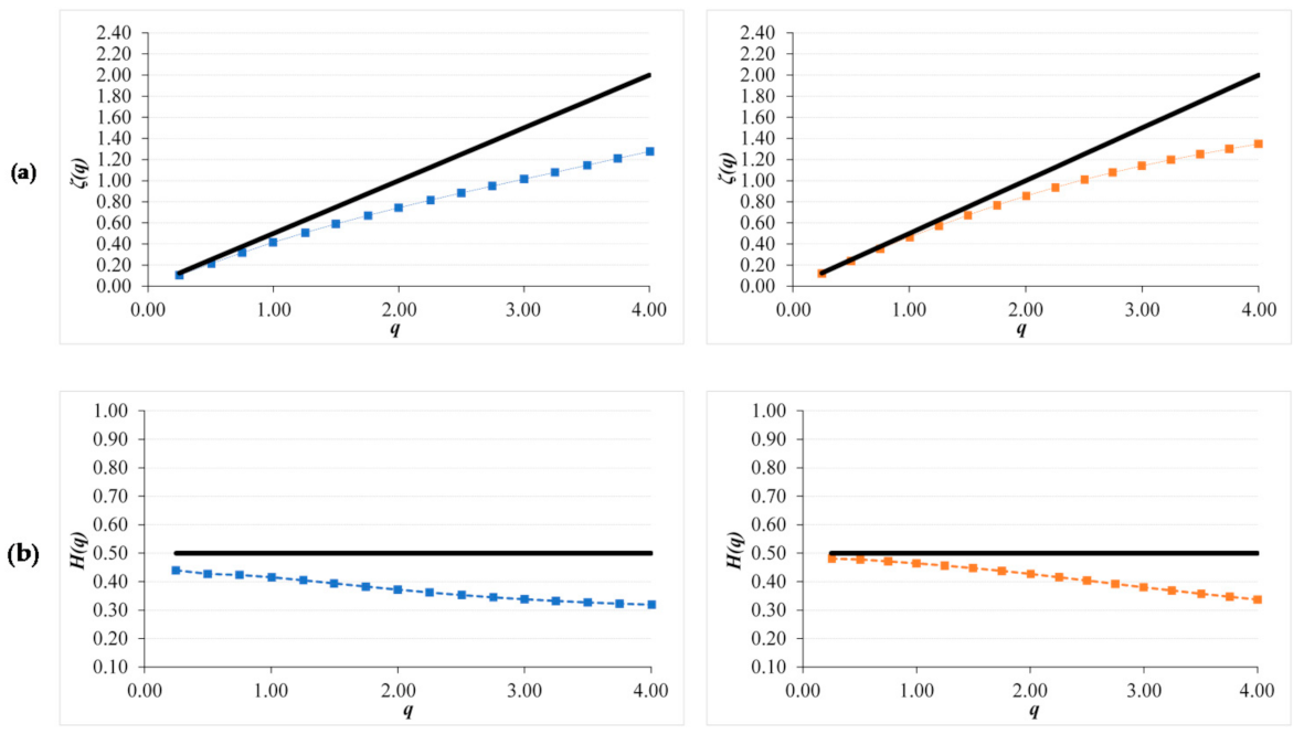
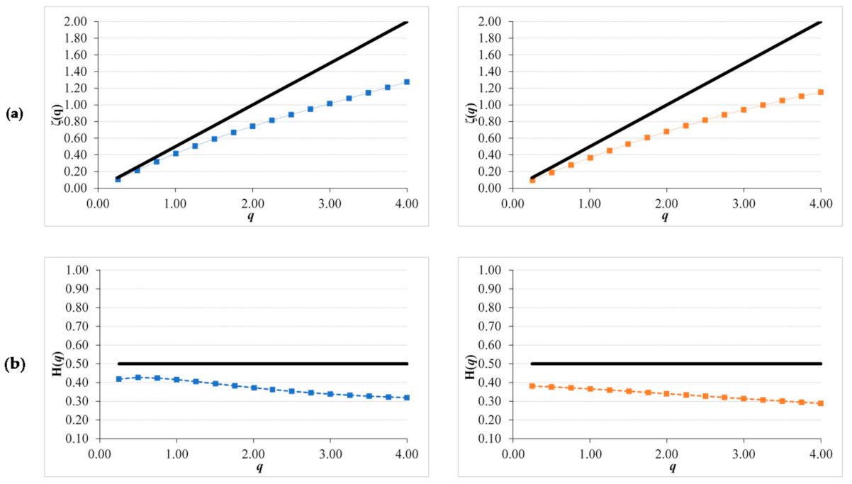
3.4. Scaling Characteristics of NDVI Residual and Anomaly Series
4. Discussion
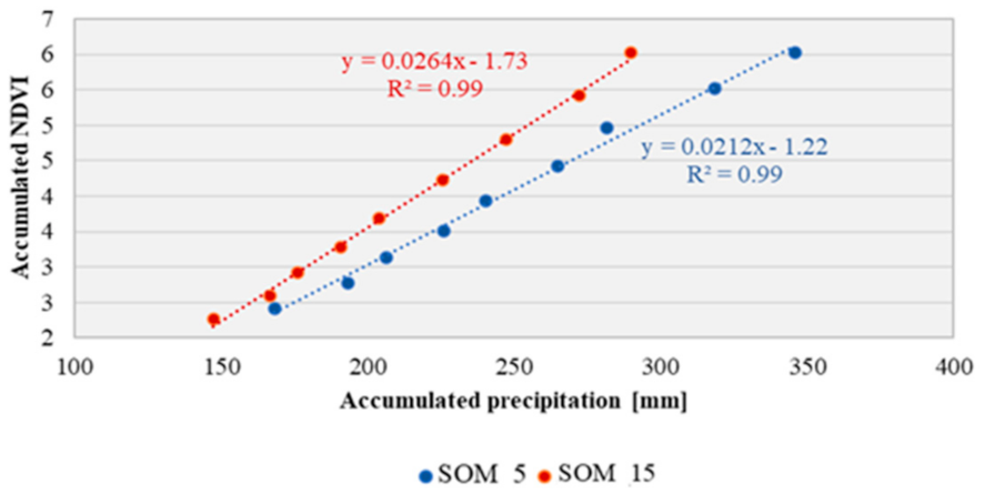
4.1. Agroclimatic Zone and NDVI Patterns
4.2. Scaling Characteristics of NDVI Original Series
4.3. Scaling Characteristics of NDVI Residual and Anomalies Series
5. Conclusions
- Data from Earth observation, in this case the MODIS satellite, through the soil reflectance differences validated the soil units from a digital soil mapping approach with the self-organizing map (SOM) algorithm.
- NDVI descriptive statistics show a significant difference between the two agroclimatic zones that mainly differ in soil physical properties and the precipitation regime.
- NDVI series exhibits a persistent structure and a clear multiscaling nature.
- When NDVI residual and anomalies series are analyzed, the pattern changes to an anti-persistent structure and a weaker multiscaling nature.
- Generalized Hurst exponents got from NDVI anomaly series can complement agroclimatic zone characterization.
Author Contributions
Funding
Institutional Review Board Statement
Informed Consent Statement
Data Availability Statement
Acknowledgments
Conflicts of Interest
Appendix A
References
- Lelièvre, F.; Norton, M.R.; Volaire, F. Perennial grasses in rainfed Mediterranean farming systems—Current and potential role. Options Méditerranéennes. Série A Séminaires Méditerranéens 2008, 79, 137–146. Available online: https://om.ciheam.org/om/pdf/a79/00800635.pdf (accessed on 12 November 2020).
- Perniola, M.; Lovelli, S.; Arcieri, M.; Amato, M. The Sustainability of Agro-Food and Natural Resource Systems in the Mediterranean Basin; Vastola, A., Ed.; Springer International Publishing: Cham, Geamany, 2015; ISBN 978-3-319-16356-7. [Google Scholar]
- Rivas-Tabares, D.; Tarquis, A.M.; Willaarts, B.; De Miguel, Á. An accurate evaluation of water availability in sub-arid Mediterranean watersheds through SWAT: Cega-Eresma-Adaja. Agric. Water Manag. 2019, 212, 211–225. [Google Scholar] [CrossRef]
- Xue, J.; Su, B. Significant remote sensing vegetation indices: A review of developments and applications. J. Sens. 2017, 2017, 1–17. [Google Scholar] [CrossRef]
- Joiner, J.; Yoshida, Y.; Anderson, M.; Holmes, T.; Hain, C.; Reichle, R.; Koster, R.; Middleton, E.; Zeng, F.-W. Global relationships among traditional reflectance vegetation indices (NDVI and NDII), evapotranspiration (ET), and soil moisture variability on weekly timescales. Remote Sens. Environ. 2018, 219, 339–352. [Google Scholar] [CrossRef] [PubMed]
- Schultz, M.; Clevers, J.G.P.W.; Carter, S.; Verbesselt, J.; Avitabile, V.; Quang, H.V.; Herold, M. Performance of vegetation indices from Landsat time series in deforestation monitoring. Int. J. Appl. Earth Obs. Geoinf. 2016, 52, 318–327. [Google Scholar] [CrossRef]
- Nagy, A.; Fehér, J.; Tamás, J. Wheat and maize yield forecasting for the Tisza river catchment using MODIS NDVI time series and reported crop statistics. Comput. Electron. Agric. 2018, 151, 41–49. [Google Scholar] [CrossRef]
- Moges, S.M.; Raun, W.R.; Mullen, R.W.; Freeman, K.W.; Johnson, G.V.; Solie, J.B. Evaluation of Green, Red, and Near Infrared Bands for Predicting Winter Wheat Biomass, Nitrogen Uptake, and Final Grain Yield. J. Plant Nutr. 2005, 27, 1431–1441. [Google Scholar] [CrossRef]
- Numata, I.; Roberts, D.A.; Chadwick, O.A.; Schimel, J.; Sampaio, F.R.; Leonidas, F.C.; Soares, J.V. Characterization of pasture biophysical properties and the impact of grazing intensity using remotely sensed data. Remote Sens. Environ. 2007, 109, 314–327. [Google Scholar] [CrossRef]
- Escribano Rodríguez, J.; Tarquis, A.M.; Saa-Requejo, A.; Díaz-Ambrona, C.G.H. Relation of NDVI obtained from different remote sensing at different space and resolutions sensors in Spanish Dehesas. In Proceedings of the EGUGA, Vienna, Austria, 12–17 April 2015; p. 15416. [Google Scholar]
- Mao, R.; Zeng, D.-H.; Li, L.-J.; Hu, Y.-L. Changes in labile soil organic matter fractions following land use change from monocropping to poplar-based agroforestry systems in a semiarid region of Northeast China. Environ. Monit. Assess. 2012, 184, 6845–6853. [Google Scholar] [CrossRef]
- Hernanz, J.L.; López, R.; Navarrete, L.; Sanchez-Giron, V. Long-term effects of tillage systems and rotations on soil structural stability and organic carbon stratification in semiarid central Spain. Soil Tillage Res. 2002, 66, 129–141. [Google Scholar] [CrossRef]
- Wu, H.; Wu, L.; Zhu, Q.; Wang, J.; Qin, X.; Xu, J.; Kong, L.; Chen, J.; Lin, S.; Khan, M.U. The role of organic acids on microbial deterioration in the Radix pseudostellariae rhizosphere under continuous monoculture regimes. Sci. Rep. 2017, 7, 1–13. [Google Scholar] [CrossRef] [PubMed]
- Vicente-Serrano, S.M. Evaluating the impact of drought using remote sensing in a Mediterranean, semi-arid region. Nat. Hazards 2007, 40, 173–208. [Google Scholar] [CrossRef]
- Lazaro, R.; Rodrigo, F.S.; Gutiérrez, L.; Domingo, F.; Puigdefábregas, J. Analysis of a 30-year rainfall record (1967–1997) in semi–arid SE Spain for implications on vegetation. J. Arid Environ. 2001, 48, 373–395. [Google Scholar] [CrossRef]
- Wang, J.; Price, K.P.; Rich, P.M. Spatial patterns of NDVI in response to precipitation and temperature in the central Great Plains. Int. J. Remote Sens. 2001, 22, 3827–3844. [Google Scholar] [CrossRef]
- Mahmoudabadi, E.; Karimi, A.; Haghnia, G.H.; Sepehr, A. Digital soil mapping using remote sensing indices, terrain attributes, and vegetation features in the rangelands of northeastern Iran. Environ. Monit. Assess. 2017, 189, 500. [Google Scholar] [CrossRef]
- Xu, Y.-T.; Zhang, Y.; Wang, S.-G. A modified tunneling function method for non-smooth global optimization and its application in artificial neural network. Appl. Math. Model. 2015, 39, 6438–6450. [Google Scholar] [CrossRef]
- Wu, J.; David, J.L. A spatially explicit hierarchical approach to modeling complex ecological systems: Theory and applications. Ecol. Modell. 2002, 153, 7–26. [Google Scholar] [CrossRef]
- Wang, X.; Wang, C.; Niu, Z. Application of R/S method in analyzing NDVI time series. Geogr. Geo-Inf. Sci. 2005, 21, 20–24. [Google Scholar]
- Peng, J.; Liu, Z.; Liu, Y.; Wu, J.; Han, Y. Trend analysis of vegetation dynamics in Qinghai–Tibet Plateau using Hurst Exponent. Ecol. Indic. 2012, 14, 28–39. [Google Scholar] [CrossRef]
- Jiang, W.; Yuan, L.; Wang, W.; Cao, R.; Zhang, Y.; Shen, W. Spatio-temporal analysis of vegetation variation in the Yellow River Basin. Ecol. Indic. 2015, 51, 117–126. [Google Scholar] [CrossRef]
- Ndayisaba, F.; Guo, H.; Bao, A.; Guo, H.; Karamage, F.; Kayiranga, A. Understanding the spatial temporal vegetation dynamics in Rwanda. Remote Sens. 2016, 8, 129. [Google Scholar] [CrossRef]
- Tong, S.; Zhang, J.; Bao, Y.; Lai, Q.; Lian, X.; Li, N.; Bao, Y. Analyzing vegetation dynamic trend on the Mongolian Plateau based on the Hurst exponent and influencing factors from 1982–2013. J. Geogr. Sci. 2018, 28, 595–610. [Google Scholar] [CrossRef]
- Hott, M.C.; Carvalho, L.M.T.; Antunes, M.A.H.; Resende, J.C.; Rocha, W.S.D. Analysis of grassland degradation in zona da Mata, MG, Brazil, based on NDVI time series data with the integration of phenological metrics. Remote Sens. 2019, 11, 2956. [Google Scholar] [CrossRef]
- Liu, X.; Tian, Z.; Zhang, A.; Zhao, A.; Liu, H. Impacts of climate on spatiotemporal variations in vegetation NDVI from 1982–2015 in Inner Mongolia, China. Sustainability 2019, 11, 768. [Google Scholar] [CrossRef]
- Davis, A.; Marshak, A.; Wiscombe, W.; Cahalan, R. Multifractal characterizations of nonstationarity and intermittency in geophysical fields: Observed, retrieved, or simulated. J. Geophys. Res. 1994, 99, 8055. [Google Scholar] [CrossRef]
- Li, X.; Lanorte, A.; Lasaponara, R.; Lovallo, M.; Song, W.; Telesca, L. Fisher–Shannon and detrended fluctuation analysis of MODIS normalized difference vegetation index (NDVI) time series of fire-affected and fire-unaffected pixels. Geomat. Nat. Hazards Risk 2017, 8, 1342–1357. [Google Scholar] [CrossRef]
- Ba, R.; Song, W.; Lovallo, M.; Lo, S.; Telesca, L. Analysis of multifractal and organization/order structure in suomi-NPP VIIRS normalized difference vegetation index series of wildfire affected and unaffected sites by using the multifractal detrended fluctuation analysis and the Fisher–Shannon analysis. Entropy 2020, 22, 415. [Google Scholar] [CrossRef]
- Rivas-Tabares, D.; De Miguel, Á.; Willaarts, B.; Tarquis, A.M. Self-Organizing Map of soil properties in the context of hydrological modeling. Appl. Math. Model. 2020. [Google Scholar] [CrossRef]
- Kohonen, T. Self-organized formation of topologically correct feature maps. Biol. Cybern. 1982, 43, 59–69. [Google Scholar] [CrossRef]
- Llera David, A.N.; Del, G.N.G.; Álvarez, P.M.V.; Cubero, A.D.; Miriam, J.; Ignacio, F.S.; Barrera, V.; García, A.G. Atlas Agroclimático de Castilla y León. Available online: http://atlas.itacyl.es/ (accessed on 10 October 2020).
- Lyon, T.L. Edafología, naturaleza y propiedades del suelo. Acme. Buenos Aires. AR 1947, 1, 117–155. [Google Scholar]
- Soil Survey Division Staff Soil Survey Manual. 1993. Available online: https://books.google.com.hk/books?hl=zh-CN&lr=&id=LYwwAAAAYAAJ&oi=fnd&pg=IA3&dq=34.%09SOIL+SURVEY+DIVISION+STAFF+Soil+survey+manual+1993&ots=7n6EAJzekd&sig=l8nYwjamdVpex0Htk71fLMblCLk&redir_esc=y#v=onepage&q&f=false (accessed on 4 February 2021).
- IGME. Identificación Y Caracterización de la Interrelación Que se Presenta Entre Aguas Subterráneas, Cursos Fluviales, Descargas Por Manantiales, Zonas Húmedas Y Otros Ecosistemas Naturales de Especial Interés Hídrico; Confederación Hidrográfica del Duero: Valladolid, Espanha, 2009; p. 66. [Google Scholar]
- Ficklin, D.L.; Stewart, I.T.; Maurer, E.P. Climate change impacts on streamflow and subbasin-scale hydrology in the Upper Colorado River Basin. PLoS ONE 2013, 8, e71297. [Google Scholar] [CrossRef]
- Kling, H.; Gupta, H. On the development of regionalization relationships for lumped watershed models: The impact of ignoring sub-basin scale variability. J. Hydrol. 2009, 373, 337–351. [Google Scholar] [CrossRef]
- Thiessen, A.H. Precipitation averages for large areas. Mon. Weather Rev. 1911, 39, 1082–1089. [Google Scholar] [CrossRef]
- Didan, K. MOD13Q1 MODIS/Terra vegetation indices 16-day L3 global 250m SIN grid V006. NASA EOSDIS L. Process. DAAC 2015. [Google Scholar] [CrossRef]
- Gorelick, N.; Hancher, M.; Dixon, M.; Ilyushchenko, S.; Thau, D.; Moore, R. Google Earth Engine: Planetary-scale geospatial analysis for everyone. Remote Sens. Environ. 2017, 202, 18–27. [Google Scholar] [CrossRef]
- Valverde-Arias, O.; Garrido, A.; Saa-Requejo, A.; Carreño, F.; Tarquis, A.M. Agro-ecological variability effects on an index-based insurance design for extreme events. Geoderma 2019, 337, 1341–1350. [Google Scholar] [CrossRef]
- Viscarra Rossel, R.A.; Cattle, S.R.; Ortega, A.; Fouad, Y. In situ measurements of soil colour, mineral composition and clay content by vis–NIR spectroscopy. Geoderma 2009, 150, 253–266. [Google Scholar] [CrossRef]
- Viscarra Rossel, R.A.; Walvoort, D.J.J.; McBratney, A.B.; Janik, L.J.; Skjemstad, J.O. Visible, near infrared, mid infrared or combined diffuse reflectance spectroscopy for simultaneous assessment of various soil properties. Geoderma 2006, 131, 59–75. [Google Scholar] [CrossRef]
- Baret, F.; Jacquemoud, S.; Hanocq, J.F. The soil line concept in remote sensing. Remote Sens. Rev. 1993, 7, 65–82. [Google Scholar] [CrossRef]
- Gitelson, A.A.; Stark, R.; Grits, U.; Rundquist, D.; Kaufman, Y.; Derry, D. Vegetation and soil lines in visible spectral space: A concept and technique for remote estimation of vegetation fraction. Int. J. Remote Sens. 2002, 23, 2537–2562. [Google Scholar] [CrossRef]
- Goslee, S.; Goslee, M.S. Package ‘landsat.’ R Packag. Doc. Available online: https//cran.r-project.org/web/packages/landsat/landsat.pdf (accessed on 16 December 2019).
- Maas, S.J.; Rajan, N. Normalizing and Converting Image DC Data Using Scatter Plot Matching. Remote Sens. 2010, 2, 1644–1661. [Google Scholar] [CrossRef]
- Yoshioka, H.; Miura, T.; Demattê, J.A.M.; Batchily, K.; Huete, A.R. Soil Line Influences on Two-Band Vegetation Indices and Vegetation Isolines: A Numerical Study. Remote Sens. 2010, 2, 545–561. [Google Scholar] [CrossRef]
- Galvão, L.S.; Vitorello, Í. Variability of Laboratory Measured Soil Lines of Soils from Southeastern Brazil. Remote Sens. Environ. 1998, 63, 166–181. [Google Scholar] [CrossRef]
- Prudnikova, E.; Savin, I.; Vindeker, G.; Grubina, P.; Shishkonakova, E.; Sharychev, D. Influence of Soil Background on Spectral Reflectance of Winter Wheat Crop Canopy. Remote Sens. 2019, 11, 1932. [Google Scholar] [CrossRef]
- Savitzky, A.; Golay, M.J.E. Smoothing and differentiation of data by simplified least squares procedures. Anal. Chem. 1964, 36, 1627–1639. [Google Scholar] [CrossRef]
- Chen, J.; Jönsson, P.; Tamura, M.; Gu, Z.; Matsushita, B.; Eklundh, L. A simple method for reconstructing a high-quality NDVI time-series data set based on the Savitzky–Golay filter. Remote Sens. Environ. 2004, 91, 332–344. [Google Scholar] [CrossRef]
- Reed, B.C.; Loveland, T.R.; Tieszen, L.L. An approach for using AVHRR data to monitor U.S. Great Plains Grasslands. Geocarto Int. 1996, 11, 13–22. [Google Scholar] [CrossRef]
- Monin, A.S.; Yaglom, A.M. Statistical Fluid Mechanics: The Mechanics of Turbulence; Massachusetts Inst of Tech Cambridge: Cambridge, MA, USA, 1999; Volume 2, p. 521. [Google Scholar]
- Lacasa, L.; Luque, B.; Luque, J.; Nuño, J.C. The visibility graph: A new method for estimating the Hurst exponent of fractional Brownian motion. EPL Europhys. Lett. 2009, 86, 30001. [Google Scholar] [CrossRef]
- Yu, C.X.; Gilmore, M.; Peebles, W.A.; Rhodes, T.L. Structure function analysis of long-range correlations in plasma turbulence. Phys. Plasmas 2003, 10, 2772–2779. [Google Scholar] [CrossRef]
- Lovejoy, S.; Schertzer, D.; Stanway, J.D. Direct evidence of multifractal atmospheric cascades from planetary scales down to 1 km. Phys. Rev. Lett. 2001, 86, 5200–5203. [Google Scholar] [CrossRef]
- Morató, M.C.; Castellanos, M.T.; Bird, N.R.; Tarquis, A.M. Multifractal analysis in soil properties: Spatial signal versus mass distribution. Geoderma 2017, 287, 54–65. [Google Scholar] [CrossRef]
- Tarquis, A.M.; Morato, M.C.; Castellanos, M.T.; Perdigones, A. Comparison of structure function and detrended fluctuation analysis of wind time series. Nuovo Cim. Della Soc. Ital. Fis. C Geophys. Sp. Phys. 2008, 31, 633–651. [Google Scholar] [CrossRef]
- Dematte, J.A.M.; Fiorio, P.R.; Ben-Dor, E. Estimation of soil properties by orbital and laboratory reflectance means and its relation with soil classification. Open Remote Sens. J. 2009, 2, 12–23. [Google Scholar] [CrossRef]
- Lobell, D.B.; Asner, G.P. Moisture effects on soil reflectance. Soil Sci. Soc. Am. J. 2002, 66, 722–727. [Google Scholar] [CrossRef]
- Kaleita, A.L.; Tian, L.F.; Hirschi, M.C. Relationship between soil moisture content and soil surface reflectance. Trans. ASAE 2005, 48, 1979–1986. [Google Scholar] [CrossRef]
- Muller, E.; Décamps, H. Modeling soil moisture–reflectance. Remote Sens. Environ. 2001, 76, 173–180. [Google Scholar] [CrossRef]
- Weidong, L.; Baret, F.; Xingfa, G.; Qingxi, T.; Lanfen, Z.; Bing, Z. Relating soil surface moisture to reflectance. Remote Sens. Environ. 2002, 81, 238–246. [Google Scholar] [CrossRef]
- Mzuku, M.; Khosla, R.; Reich, R. Bare soil reflectance to characterize variability in soil properties. Commun. Soil Sci. Plant Anal. 2015, 46, 1668–1676. [Google Scholar] [CrossRef]
- Smith, R.; Adams, J.; Stephens, D.; Hick, P. Forecasting wheat yield in a Mediterranean-type environment from the NOAA satellite. Aust. J. Agric. Res. 1995, 46, 113. [Google Scholar] [CrossRef]
- Martínez, B.; Gilabert, M.A. Vegetation dynamics from NDVI time series analysis using the wavelet transform. Remote Sens. Environ. 2009, 113, 1823–1842. [Google Scholar] [CrossRef]
- Al-Bakri, J.T.; Suleiman, A.S. NDVI response to rainfall in different ecological zones in Jordan. Int. J. Remote Sens. 2004, 25, 3897–3912. [Google Scholar] [CrossRef]
- Liu, H.Q.; Huete, A. A feedback based modification of the NDVI to minimize canopy background and atmospheric noise. IEEE Trans. Geosci. Remote Sens. 1995, 33, 457–465. [Google Scholar] [CrossRef]
- Igbawua, T.; Zhang, J.; Yao, F.; Ali, S. Long range correlation in vegetation over West Africa from 1982 to 2011. IEEE Access 2019, 7, 119151–119165. [Google Scholar] [CrossRef]
- Lovejoy, S.; Tarquis, A.M.; Gaonac’h, H.; Schertzer, D. Single- and multiscale remote sensing techniques, multifractals, and MODIS-derived vegetation and soil moisture. Vadose Zo. J. 2008, 7, 533–546. [Google Scholar] [CrossRef]
- Duffaut Espinosa, L.A.; Posadas, A.N.; Carbajal, M.; Quiroz, R. Multifractal downscaling of rainfall using normalized difference vegetation index (NDVI) in the Andes plateau. PLoS ONE 2017, 12, e0168982. [Google Scholar] [CrossRef]
- Alonso, C.; Tarquis, A.M.; Zúñiga, I.; Benito, R.M. Spatial and radiometric characterization of multi-spectrum satellite images through multi-fractal analysis. Nonlin. Process. Geophys. 2017, 24, 141–155. [Google Scholar] [CrossRef]
- Martín-Sotoca, J.J.; Saa-Requejo, A.; Borondo, J.; Tarquis, A.M. Singularity maps applied to a vegetation index. Biosyst. Eng. 2018, 168, 42–53. [Google Scholar] [CrossRef]


| SOM Unit | SOM_05 | SOM15 |
|---|---|---|
| Slope [%] | 1–16 | 1–17 |
| Altitude [MASL] | 925–1050 | 888–912 |
| Clay [%] | 29 (5.2) | 4 (3) |
| Sand [%] | 56 (4.6) | 84 (3.9) |
| Silt [%] | 14 (4.4) | 12 (3.5) |
| Organic Matter [%] | 0.9 (0.10) | 1.7 (0.15) |
| Bulk density [g/cm3] | 1420 (145) | 1839 (129) |
| Carbon content [%] | 0.5 (0.08) | 1.0 (0.09) |
| Available water content [mm H2O] | 10.1 (0.7) | 5.8 (0.7) |
| Hydraulic Conductivity [mm/hr] | 150 (88) | 2890 (981) |
| Soil moist albedo [ratio] | 0.08 (0.010) | 0.03 (0.005) |
| Effective Soil depth [mm] | 1100 | 825 |
| OCT | NOV | DIC | JAN | FEB | MAR | APR | MAY | JUN | JUL | AUG | SEPT | Annual Values | |
|---|---|---|---|---|---|---|---|---|---|---|---|---|---|
| Sub-basin 50 (SOM5) | |||||||||||||
| Pcp [mm] | 67.1 | 59.7 | 40.1 | 52.3 | 39.0 | 40.7 | 56.1 | 57.0 | 31.7 | 14.5 | 13.8 | 27.1 | 499.1 |
| Tmax [°C] | 18.2 | 11.0 | 8.3 | 8.0 | 9.4 | 13.0 | 15.6 | 20.2 | 26.9 | 30.2 | 30.1 | 25.6 | 18.0 |
| Tavg [°C] | 12.8 | 6.9 | 4.4 | 4.0 | 4.6 | 7.4 | 9.4 | 13.0 | 18.8 | 21.3 | 21.7 | 18.1 | 11.9 |
| Tmin [°C] | 7.3 | 2.8 | 0.4 | 0.0 | −0.1 | 1.8 | 3.2 | 5.8 | 10.6 | 12.5 | 13.3 | 10.6 | 5.7 |
| Sub-basin 24 (SOM15) | |||||||||||||
| Pcp [mm] | 61.2 | 45.5 | 34.2 | 36.5 | 30.7 | 36.0 | 50.3 | 50.5 | 31.2 | 12.6 | 16.4 | 25.3 | 430.4 |
| Tmax [°C] | 17.9 | 11.0 | 8.3 | 8.1 | 9.4 | 12.8 | 15.4 | 20.0 | 26.8 | 30.0 | 29.9 | 25.4 | 17.9 |
| Tavg [°C] | 12.6 | 6.9 | 4.4 | 3.9 | 4.6 | 7.2 | 9.2 | 12.8 | 18.5 | 21.0 | 21.4 | 17.9 | 11.7 |
| Tmin [°C] | 7.2 | 2.8 | 0.4 | −0.2 | −0.2 | 1.6 | 3.0 | 5.7 | 10.2 | 12.1 | 12.8 | 10.4 | 5.5 |
| Reflectance Bands | ||||||||
|---|---|---|---|---|---|---|---|---|
| NIR | RED | Blue | MIR | |||||
| SOM soil unit | 5 | 15 | 5 | 15 | 5 | 15 | 5 | 15 |
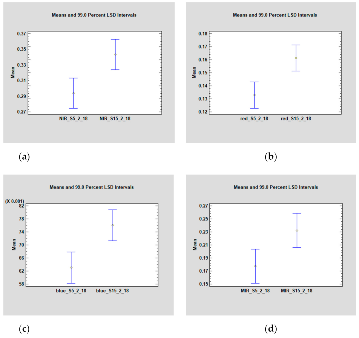
| Mean | 0.294 | 0.343 | 0.133 | 0.161 | 0.063 | 0.076 | 0.177 | 0.232 |
| Typical error | 0.009 | 0.011 | 0.004 | 0.006 | 0.002 | 0.003 | 0.011 | 0.016 |
| Median | 0.290 | 0.332 | 0.136 | 0.161 | 0.064 | 0.076 | 0.185 | 0.222 |
| Standard deviation | 0.038 | 0.051 | 0.018 | 0.028 | 0.010 | 0.012 | 0.049 | 0.071 |
| Kurtosis | −0.553 | −0.707 | −0.122 | −0.906 | −0.548 | −0.636 | −1.184 | −0.421 |
| Skewness | 0.005 | 0.412 | −0.607 | 0.006 | −0.229 | −0.217 | −0.331 | 0.583 |
| Count | 20 | 20 | 20 | 20 | 20 | 20 | 20 | 20 |
| Normality test | ||||||||
| Shapiro–Wilk | ||||||||
| Statistic | 0.932 | 0.922 | 0.955 | 0.965 | 0.971 | 0.973 | 0.964 | 0.959 |
| P-value | 0.170 | 0.108 | 0.442 | 0.644 | 0.971 | 0.808 | 0.624 | 0.523 |
| Kolmogorov–Smirnov | ||||||||
| P-value | 0.776 | 0.749 | 0.932 | 0.898 | 0.934 | 0.912 | 0.969 | 0.987 |
| Source | Sum of Squares | Degrees of Freedom | Mean Square | F-Ratio | p-Value |
|---|---|---|---|---|---|
| NIR | |||||
| Between SOMs | 0.024 | 1 | 0.024 | 11.93 | 0.001 |
| Within SOMs | 0.078 | 38 | 0.002 | ||
| Total (corrected) | 0.103 | 39 | |||
| Red | |||||
| Between SOMs | 0.008 | 1 | 0.008 | 14.67 | 0.001 |
| Within SOMs | 0.021 | 38 | 0.001 | ||
| Total (corrected) | 0.029 | 39 | |||
| Blue | |||||
| Between SOMs | 0.002 | 1 | 0.002 | 13.51 | 0.001 |
| Within SOMs | 0.005 | 38 | 0.000 | ||
| Total (corrected) | 0.006 | 39 | |||
| MIR | |||||
| Between SOMs | 0.030 | 1 | 0.030 | 8.03 | 0.007 |
| Within SOMs | 0.142 | 38 | 0.004 | ||
| Total (corrected) | 0.172 | 39 |
| Source | Sum of Squares | Df | Mean Square | F-Ratio | p-Value |
|---|---|---|---|---|---|
| Intercepts | 0.0016 | 1 | 0.0016 | 79.53 | 0.0000 |
| Slopes | 0.0001 | 1 | 0.0001 | 4.46 | 0.0383 |
| Source | Sum of Squares | Degrees of Freedom | Mean Square | F-Ratio | p-Value |
|---|---|---|---|---|---|
| NDVI | |||||
| Between SOMs | 0.112 | 1 | 0.112 | 10.15 | 0.002 |
| Whitin SOMs | 2.635 | 238 | 0.011 | ||
| Total (corrected) | 2.747 | 239 |
| Zone | NDVI Series | H(q = 1) | H(q = 2) | ΔH(q) |
|---|---|---|---|---|
| SOM5 | Original | 0.78 | 0.70 | 0.40 |
| Residual | 0.41 | 0.37 | 0.12 | |
| anomaly | 0.40 | 0.37 | 0.09 | |
| SOM15 | Original | 0.80 | 0.70 | 0.40 |
| Residual | 0.46 | 0.43 | 0.14 | |
| anomaly | 0.37 | 0.34 | 0.09 |
Publisher’s Note: MDPI stays neutral with regard to jurisdictional claims in published maps and institutional affiliations. |
© 2021 by the authors. Licensee MDPI, Basel, Switzerland. This article is an open access article distributed under the terms and conditions of the Creative Commons Attribution (CC BY) license (http://creativecommons.org/licenses/by/4.0/).
Share and Cite
Rivas-Tabares, D.A.; Saa-Requejo, A.; Martín-Sotoca, J.J.; Tarquis, A.M. Multiscaling NDVI Series Analysis of Rainfed Cereal in Central Spain. Remote Sens. 2021, 13, 568. https://doi.org/10.3390/rs13040568
Rivas-Tabares DA, Saa-Requejo A, Martín-Sotoca JJ, Tarquis AM. Multiscaling NDVI Series Analysis of Rainfed Cereal in Central Spain. Remote Sensing. 2021; 13(4):568. https://doi.org/10.3390/rs13040568
Chicago/Turabian StyleRivas-Tabares, David Andrés, Antonio Saa-Requejo, Juan José Martín-Sotoca, and Ana María Tarquis. 2021. "Multiscaling NDVI Series Analysis of Rainfed Cereal in Central Spain" Remote Sensing 13, no. 4: 568. https://doi.org/10.3390/rs13040568
APA StyleRivas-Tabares, D. A., Saa-Requejo, A., Martín-Sotoca, J. J., & Tarquis, A. M. (2021). Multiscaling NDVI Series Analysis of Rainfed Cereal in Central Spain. Remote Sensing, 13(4), 568. https://doi.org/10.3390/rs13040568