Article

Automatic High-Accuracy Sea Ice Mapping in the Arctic Using MODIS Data

1
Aerospace Information Research Institute, Chinese Academy of Sciences, Beijing 100094, China
2
School of Electronic, Electrical and Communication Engineering, University of Chinese Academy of Sciences, Beijing 100049, China
*
Author to whom correspondence should be addressed.
Remote Sens. 2021, 13(4), 550; https://doi.org/10.3390/rs13040550
Submission received: 12 December 2020 / Revised: 27 January 2021 / Accepted: 2 February 2021 / Published: 4 February 2021
(This article belongs to the Special Issue Application of MODIS Data for Environmental Research)

Abstract

:
The sea ice cover is changing rapidly in polar regions, and sea ice products with high temporal and spatial resolution are of great importance in studying global climate change and navigation. In this paper, an ice map generation model based on Moderate-Resolution Imaging Spectroradiometer (MODIS) reflectance bands is constructed to obtain sea ice data with a high temporal and spatial resolution. By constructing a training sample library and using a multi-feature fusion machine learning algorithm for model classification, the high-accuracy recognition of ice and cloud regions is achieved. The first product provided by this algorithm is a near real-time single-scene sea ice presence map. Compared with the photo-interpreted ground truth, the verification shows that the algorithm can obtain a higher recognition accuracy for ice, clouds, and water, and the accuracy exceeds 98%. The second product is a daily and weekly clear sky map, which provides synthetic ice presence maps for one day or seven consecutive days. A filtering method based on cloud motion is used to make the product more accurate. The third product is a weekly fusion of clear sky optical images. In a comparison with the Advanced Microwave Scanning Radiometer 2 (AMSR2) sea ice concentration products performed in August 2019 and September 2020, these composite images showed spatial consistency over time, suggesting that they can be used in many scientific and practical applications in the future.

Graphical Abstract

1. Introduction

With the onset of global warming in recent years, the melting rate of polar sea ice has accelerated since the late 1970s [1]. According to a report by the National Snow and Ice Data Center (NSIDC), the Arctic sea ice extent reached its second lowest value in history on September 2020, behind only September 2012 [2]. Sea ice plays an important role in the study of global climate change [3,4,5] and biodiversity [6]. Sea ice monitoring will help us to better understand the impact of climate change on species’ habitats. In addition, with the increasing frequency of maritime economic activities and traffic in the Arctic, the demand for sea ice information monitoring is also increasing rapidly [7,8,9,10,11]. The increasing rate of sea ice melting has put the navigation of the Arctic waterway on the agenda, and sea ice information with a high spatial and temporal resolution will help us to accurately judge sea routes.
Passive microwave data are not affected by clouds and can form daily global coverage observations, but their spatial resolution is low and most of them are kilometer-level products [12,13,14,15,16,17]. The existing sea ice concentration (SIC) data products mostly rely on passive microwave radiometer data. The University of Bremen in Germany released an SIC product with a spatial resolution of 6.25 km based on the AMSR2 sensor using the ARTIST Sea Ice (ASI) algorithm, and another SIC product with a spatial resolution of 12.5 km using the Bootstrap algorithm [15]. The University of Hamburg released an SIC product with a spatial resolution of 3.125 km based on the AMSR2 sensor using the ASI algorithm [15,18]. The NSIDC released an SIC product with a spatial resolution of 25 km based on the sensors of Scanning Multichannel Microwave Radiometer (SMMR) and Special Sensor Microwave Imager/Sounder (SSMIS) using the Bootstrap algorithm [19] and another SIC product with a spatial resolution of 25 km based on the SSMIS sensor using the NASA Team (NT) algorithm [17]. The European Organization for the Exploitation of Meteorological Satellites (EUMETSAT) released a product with a spatial resolution of 10 km based on the SSMIS sensor using the algorithm combined with Bristol and Bootstrap [20,21].
SAR images have the characteristics of being all-day and all-weather and having a high spatial resolution, and can provide high-quality sea ice information [22,23,24,25,26,27]. Currently, the SAR data used for sea ice monitoring mainly include the Radarsat-2 and Sentinel-1A satellite data, which can obtain a good spatial resolution [28,29]. Boulze et al. [28] proposed a sea ice classification using convolutional neural networks for Sentinel-1 data and obtained good classification results. The phase difference of the Radarsat-2 data can be used to identify the edge ice area well [29]. SAR data are the main source of information production on the National Ice Service operational map products, but there is no mature operational quantitative algorithm for sea ice concentration inversion [30]. Moreover, due to their long revisit cycle and small coverage, it is difficult to provide large-scale daily sea ice data.
Optical satellite sensors can provide remote sensing data with a high spatial and temporal resolution and can obtain rich detailed information on ground features, despite the great influence of cloud cover and daylight conditions. It is possible to more accurately estimate the presence of sea ice in narrow passages and archipelagos areas in the polar regions [31]. The spectral and local texture characteristics of ice, snow, and clouds are very similar, which makes it difficult to distinguish them in polar regions [31,32]. At present, for the recognition of ice and clouds, the threshold segmentation method is more mature. Choi et al. [33] improved the accuracy of cloud area recognition by automatically determining the Normalized Difference Snow Index (NDSI) threshold judgment algorithm and cloud shadow matching technology. Similarly, the Normalized Difference Snow and Ice Index-1 (NDSII-1) and the Normalized Difference Snow and Ice Index-2 (NDSII-2) ice and snow indices, which use the difference in ice and snow reflectance, have been proposed [34,35]. The traditional cloud recognition method based on a multi-channel threshold is relatively easy to perform, but it is difficult to determine an appropriate threshold for them, especially for recognizing the difference between snow and clouds. Thin clouds and broken ice are often confused for each other. Machine learning methods have been applied to cloud and ice detection, but there is no mature technology for sea ice operational map products [36,37,38]. Zhan et al. [36] proposed a deep learning system for cloud and snow classification based on pixel-level fully convolutional neural networks. Varshney et al. [37] used a convolutional neural network to distinguish between clouds and snow pixels from the shortwave infrared sensor data of the ResourceSat-2 satellite. Ghasemian et al. [38] proposed two cloud detection methods, Feature Level Fusion Random Forest and Decision Level Fusion Random Forest, based on machine learning and multi-feature fusion, respectively.
The MODIS sensors can achieve multiple observations per day in the polar regions, and the spatial resolution of the data acquired is much higher than that of passive microwave data, thus they have great potential for retrieving ice maps with a higher spatial and temporal resolution. The MOD29 products [39] provided on the NASA website are prone to misjudgment in the detection of new ice in areas where ice and water are mixed, as well as areas where clouds appear over ice or water. This is mainly because the MOD29 ice products use MOD35 cloud cover products with a poor recognition accuracy in polar regions, especially in ice areas covered by clouds, thin clouds, or fog. The MOD35 products have a higher accuracy in the summer and a lower recognition accuracy in the winter, and are highly dependent on the surface type and solar illumination in the Arctic region. The MOD35 products tend to underestimate cloud cover over sea ice and overestimate cloud cover over open waters [31,40]. Charles et al. [31] proposed a hybrid cloud mask based on the MOD35 products and visible-band products, using the decision tree classification method to depict the ice map, but its sea ice detection accuracy is limited by the accuracy of the cloud mask data used.
In this study, an ice mapping method with a high accuracy and high spatial–temporal resolution is proposed that can provide three products, including single-scene ice presence maps, daily or weekly ice presence maps, and the weekly fusion of clear sky optical images. We first constructed a training sample library based on MODIS reflectance data and then used a Multi-Feature Level Fusion Random Forest (MFLFRF) algorithm to train the model and generate cloud and ice recognition results. Finally, we obtained daily and weekly composite ice maps and fusion images of the Arctic using a filtering method based on cloud motion and weighted fusion method. This proposed algorithm can provide sea ice presence maps with an improved accuracy due to its finer spatial resolution. Additionally, these improvements can achieve a near real-time monitoring of sea ice on a finer scale.

2. Materials and Methods

2.1. Data

2.1.1. MODIS Sensors and Datasets

The Terra satellite was launched into a polar orbit on December 18, 1999, with equatorial crossing at 10:30 a.m. local time every day. The Aqua satellite was launched into a polar orbit on 4 May 2002, with equatorial crossing at 1:30 p.m. local time every day. The technical performance provided by Terra is similar to that of Aqua. The two satellites observe the Earth’s surface every one or two days, and the ground repetition period is 16 days. The Moderate-Resolution Imaging Spectroradiometer (MODIS), which is carried on the Terra and Aqua satellites, has a 2330 km swath and 36 spectral bands. The spatial resolution of bands 1–2 is 250 m, bands 3–7 have a spatial resolution of 500 m, and other bands have a spatial resolution of 1000 m. Table 1 shows the spatial and spectral characteristics of MODIS reflection bands 1–7.
The data obtained by the MODIS sensors in these two satellites can be downloaded from the NASA website (https://search.earthdata.nasa.gov/search) for free. In this study, the L1B data of MODIS collection 6 products were selected to generate composite ice presence maps of the Arctic region. Taking the MODIS-Terra satellite as an example, the data used are as follows. Similarly, the prefix of the MODIS-Aqua satellite product file name is MYD, and MOD is the one of MODIS-Terra.
MOD021KM: MODIS-Terra 1 km data;
MOD02HKM: MODIS-Terra 500 m data;
MOD02QKM: MODIS-Terra 250 m data.
This study selected the L1B data of the Aqua and Terra satellites covering the Arctic in August 2019 and September 2020 to evaluate the algorithm. The comparison data selected the MOD29 products from the NASA website, and the SIC products from the AMSR2 data from the University of Bremen, Germany (https://seaice.uni-bremen.de/data/). The MOD29 products have a spatial resolution of 1 km, and the SIC products from AMSR2 have a spatial resolution of 6.25 km. All the data use the WGS84 polar stereographic projection. The MOD29 products are classified images consisting of four surface types: water, ice, cloud, and land.

2.1.2. Land Mask

In the polar regions, the MODIS sea ice reflectance MOD29 products have more accurate land area data. This study extracted the land area from the MOD29 data on 3 August 2019, and the nearest distance method was used to resample it to a spatial resolution of 250 m. As the coastline changes extremely slowly, it can be regarded as stable for a long time. Therefore, the extracted data of this day is used as the land mask data in this study.

2.2. Method

This research proposes a machine learning algorithm based on multiple feature-level fusion to automatically classify single-scene images to generate the first ice presence map products. On the basis of the above products, a filtering based on cloud motion and weighted fusion method is proposed that can automatically generate the daily/weekly composite ice presence maps and weekly fused optical images. The methodological framework is shown in Figure 1 and described in the following three subsections: pre-processing (Section 2.2.1), classification by MFLFRF algorithm (Section 2.2.2), and composite ice presence maps (Section 2.2.3).

2.2.1. Pre-Processing

After downloading the data of the research area from the NASA website, the required bands in the image were geometrically corrected and reprojected to the WGS84 polar stereographic projection. This process can be completed in batches by calling the HDF-EOS To GeoTIFF Conversion Tool (HEG) (https://wiki.earthdata.nasa.gov/display/DAS/Downloads), which is special processing tool used for MODIS images. Then, cropping, resampling of the nearest distance, radiometric calibration, solar zenith angle correction, and land mask processing on the image of the study area were performed. The radiometric calibration and solar zenith angle correction formulas are as follows:
  • Radiometric calibration:
The formula for apparent reflectance calculation [41,42,43]:
R B , T , F S = R e f l e c t a n c e _ S c a l e B × ( S I B , T , F S R e f l e c t a n c e _ O f f s e t B ) .
In this equation, R B , T , F S is the reflectance of each pixel in the corresponding band, where B is the corresponding band, T is the track, and F S is the frame_and_sample; S I B , T , F S is the count values of a single pixel in the corresponding band; R e f l e c t a n c e _ S c a l e B is the reflectance scaling ratio; R e f l e c t a n c e _ O f f s e t B is the reflectance offset. After absolute radiometric calibration, the unit of radiance is W/(m2·μm·sr), and these parameters can be read in the attribute domain of the scientific data set of the corresponding band.
  • Solar zenith angle correction:
The solar zenith angle data obtained from the MOD021KM of the MODIS data is interpolated to a 250 m spatial resolution using the shortest distance method. Then, the resampled data of the solar zenith angle are calculated according to the correction formula of the solar zenith angle. The correction formula of the solar zenith angle is as follows [41,42,43]:
Z s = D N × S _ S c a l e × π ÷ 180 ,
S R B , T , F S = ( R B , T , F S ) ÷ c o s ( Z s ) .
Then, we combine the two formulas into:
S R B , T , F S = ( R B , T , F S ) ÷ c o s ( D N × S _ S c a l e × π ÷ 180 ) ,
where Z s is the solar zenith angle (radians) corresponding to each pixel; D N is the detection value of the solar zenith angle of each pixel; S _ S c a l e is the scaling ratio between the probe value and the real value, which is 0.01 by default. S R B , T , F S is the apparent reflectance of a single pixel in the corresponding band after the solar zenith angle is corrected.
  • Feature attribute selection:
Snow and ice have a strong reflectance in visible (VIR), and a strong absorption in near infrared (NIR) and shortwave infrared (SWIR). This combination of bands makes the distinction between ice, clouds, and sea water more obvious. The thick ice and snow present a bright sky blue, while the cloud layer composed of small water droplets has the same scattering in visible light and short-wave infrared bands and its color appears white. These clouds usually exist lower, near the ground, and have higher temperatures. High and cold clouds are mostly composed of small ice crystals, which appear blue, while water clouds appear white. Therefore, the false color combinations of bands 7, 2, and 1 are selected to identify ice and clouds in the Arctic region in this study.
The NDSI utilizes the contrast spectral behavior of the visible (green band 4: 0.55 μm) and shortwave infrared (SWIR band 6: 1.64 μm) part of the spectrum [31,44]. Since the reflectance of snow in the green band and shortwave infrared band shows a strong contrast, the two bands can be used to extract ice and snow well. Therefore, using the NDSI index is a classic way to distinguish sea ice from other surface features [31,45].
N D S I = ( G r e e n S W I R ) ÷ ( G r e e n + S W I R ) .
The NDSII-1 [34] and the NDSII-2 [35] are the same as the NDSI, which is realized by using the difference in reflectance of ice and snow, but uses different spectral bands to express the reflectivity of ice and snow. In order to improve the accuracy of the overall sea ice map, the NDSII-2 index was selected in this study, as it can identify sea ice more accurately than other indices [31,35].
N D S I I 1 = ( R e d S W I R ) ÷ ( R e d + S W I R ) ,
N D S I I 2 = ( G r e e n N I R ) ÷ ( G r e e n + N I R ) .
Sea ice and clouds have similar characteristics in the spectrum, and it is very difficult to distinguish them only by their spectral features. Texture features can describe the spatial distribution of spectral information [38,46]. Some scholars have used the difference in texture features in the visible band for cloud detection [38,45]. The traditional Local Binary Pattern (LBP) operator describes the local spatial structure of an image [38,47]. It encodes the difference between the center pixel x c and its neighboring pixels into a binary pattern, and uses the binary pattern to mark the center pixel. The shape of the adjacent area is circular, and the radius is r .
L B P r , p ( x c ) = n = 0 p 1 s ( x r , p , n x c ) 2 n ,     s ( x ) = { 1     x 0   0     x < 0 ,
where p is the number of neighborhood pixels on the circumference of a circle and s (   ) is a step function.
In order to improve the robustness of the operator to noise, Liu et al. [48] proposed a Robust Extended Local Binary Pattern (RELBP) texture descriptor. This operator takes into account the influence of the intensity of the center pixel and the filter response of the image. RELBP contains three descriptors, which are RELBP_CI, based on the intensity difference of the center pixel; RELBP_NI, based on the intensity difference of neighboring pixels; and RELBP_RD, based on the radial pixel intensity difference. The RELBP_CI descriptor is selected in this study, and the formula is as follows:
R E L B P _ C I ( x c ) = s ( ( X c , ω ) μ ω ) ,
where X c , ω is a local patch of size ω × ω and its center is in location x c . (   ) is the filter applied to the patch. The median filter is selected in this paper. μ ω is the mean of ( X c , ω ) over the whole image [38,48].

2.2.2. Classification Using the MFLFRF Algorithm

Combining the spectral and textural features of ice and clouds in the polar regions, a Multi-Feature Level Fusion Random Forest (MFLFRF) classification algorithm was constructed to classify the ground objects into three types of targets: cloud, ice, and water. The Random Forest (RF) classification algorithm based on ensemble learning has become one of the most widely used algorithms in remote sensing and other application fields [49,50,51]. The RF classification algorithm is based on the decision tree as the basic unit. Through ensemble learning, multiple decision tree weak classifiers are formed into a strong classifier. The final decision category is determined by voting on the classification results of all weak classifiers. RF is a general term for ensemble methods using tree-type classifiers, which are independent learning and prediction [51]. The base classifier in the RF algorithm is the classification and regression tree (CART) decision tree. Each decision tree is trained on the training samples of the original training data, and only a subset of the input variables randomly selected by each node can be searched to determine the segmentation, which makes its training time shorter than that of other ensemble methods [50].
  • Construction of training sample library:
In the traditional RF classification method, it is necessary to individually select training samples for each image for classification. However, this would be very complicated for the batch production of cloudless sea ice products. The types of surface features are relatively simple in the Arctic region and include clouds, open water, and sea ice. The regional features of the ground features are relatively fixed and are less affected by seasons and other factors, so it is possible to reuse the samples. Therefore, this study developed a training sample library to classify surface features in the Arctic through model training and prediction. The training samples were selected from the whole Arctic region by uniform sampling. The sample categories include sea ice, water, and clouds. The texture of clouds is random and is determined by the type of cloud. Thick clouds tend to be massive and their texture is relatively rough. The texture of thin clouds such as cirrus clouds is smoother and is quite different from the texture of ice and snow. According to different cloud texture and color characteristics, the cloud region samples were divided into cloud 1, cloud 2, and cloud 3, until they were finally classified as a cloud sample. Eighty percent of them were used as training samples, and the remaining twenty percent were used as validation samples. The details of the training sample library are shown in Table 2.
  • Classification Method Details:
The three common spectral bands (bands 7, 2, and 1), as well as the four calculated indices (NDSII-2, the texture features of bands 7, 2, and 1, respectively) were used as input features for the RF classification process. The pixel-based classification model was trained using the unified training samples. There are two important parameters that should be controlled to acquire a better classification result in the RF function: number of trees to grow (ntree) and number of variables randomly sampled as candidates at each split (mtry). Since the RF classifier is computationally efficient and does not overfit, the number of trees can be as large as possible [49]. However, when the number of trees is increased above a threshold, the classification is no longer improved, as some studies on the sensitivity of RF classifiers based on the number of trees have proved [51,52]. The default value of ntree for remote sensing image prediction is 500. A higher mtry will result in stronger individual decision trees, but with an increase in correlation between trees, the accuracy of the model is reduced [50]. An mtry usually uses the square root of the total number of variables in classification tasks [38]. The two parameters ntree and mtry were determined with a test based on the modified out-of-bag (M-OOB) accuracy in this study, and we found that the number of 500 for ntree and four for mtry worked well for the classification task.

2.2.3. Composite Ice Presence Maps

By synthesizing the classification results of Aqua and Terra satellite images taken on the same day in the Arctic, a daily ice presence map was obtained, and a weekly ice presence map and a weekly fusion optical image were obtained based on this. The following rules were formulated in the composite ice maps:
  • Calculate the number of times N of non-cloud categories for each pixel among all image classification results from the Terra or Aqua satellites in a day.
  • (1) Ice extraction: Judge whether N is greater than the threshold T1. T1 is the threshold of the number of ice occurrences for each pixel per day and was defined as 5 in this study. If N is greater than T1, the pixel is judged to be in the category corresponding to the mode of the non-cloud sequence, and ice extraction is performed on the entire Arctic region. If N is less than T1, the pixel is judged to be a cloud. (2) Water extraction: Determine whether N is greater than the threshold T2. T2 is the threshold of the number of water occurrences for each pixel per day and was defined as 2 in this study. If N is greater than T2, the pixel is judged to be in the category corresponding to the mode of the non-cloud sequence, and water extraction is performed on the entire Arctic region; if N is less than T2, the pixel is judged to be a cloud.
  • Synthesize the results extracted in step 2 to obtain daily synthetic ice maps.
  • Repeat steps 1 to 3 to calculate the ice map for seven consecutive days and synthesize the final ice map for the week.
  • Use all daily synthetic ice maps for seven consecutive days to correct the classification results of the MFLFRF algorithm. According to the corrected classification results, the pre-processed images are fused by assigning weights to obtain weekly fused images.
  • The specific processing flow is shown in Figure 2.
  • Daily and weekly composite ice presence maps:
In the classification results using the MFLFRF algorithm, the extracted sea ice is mixed with a little cloud and cloud shadow, while the accuracy of the water extraction is higher. Therefore, when performing ice map synthesis, ice and water are extracted separately. First, the number of non-cloud categories N that the current pixel appears in all image classification results obtained from the Terra or Aqua satellites in a day is calculated, and then the category of the current pixel is determined by comparing N with the threshold to extract ice and water regions. In this way, it can be ensured that the area of the ice map can be maximized under the given cloud cover.
  • Weekly fused images:
Since the shortwave infrared band has the characteristics of penetrating thin clouds but cannot penetrate thick clouds, the thin cloud areas can be extracted by threshold segmentation using band 7. After normalizing the thin cloud areas, the power function formula y = ( 1 x ) 4 is used to calculate the weight of the thin cloud areas. Here, x represents the normalized pixel value of the thin cloud, and y is the assigned weight value. The weight value range is between 0 and 1, and the smaller the thin cloud value, the larger the weight value assigned. Then, the weighted average value of each pixel is calculated to obtain the weekly fusion image.

3. Results

3.1. Results of the Ice Map Products

3.1.1. The Single-Scene Ice Presence Maps

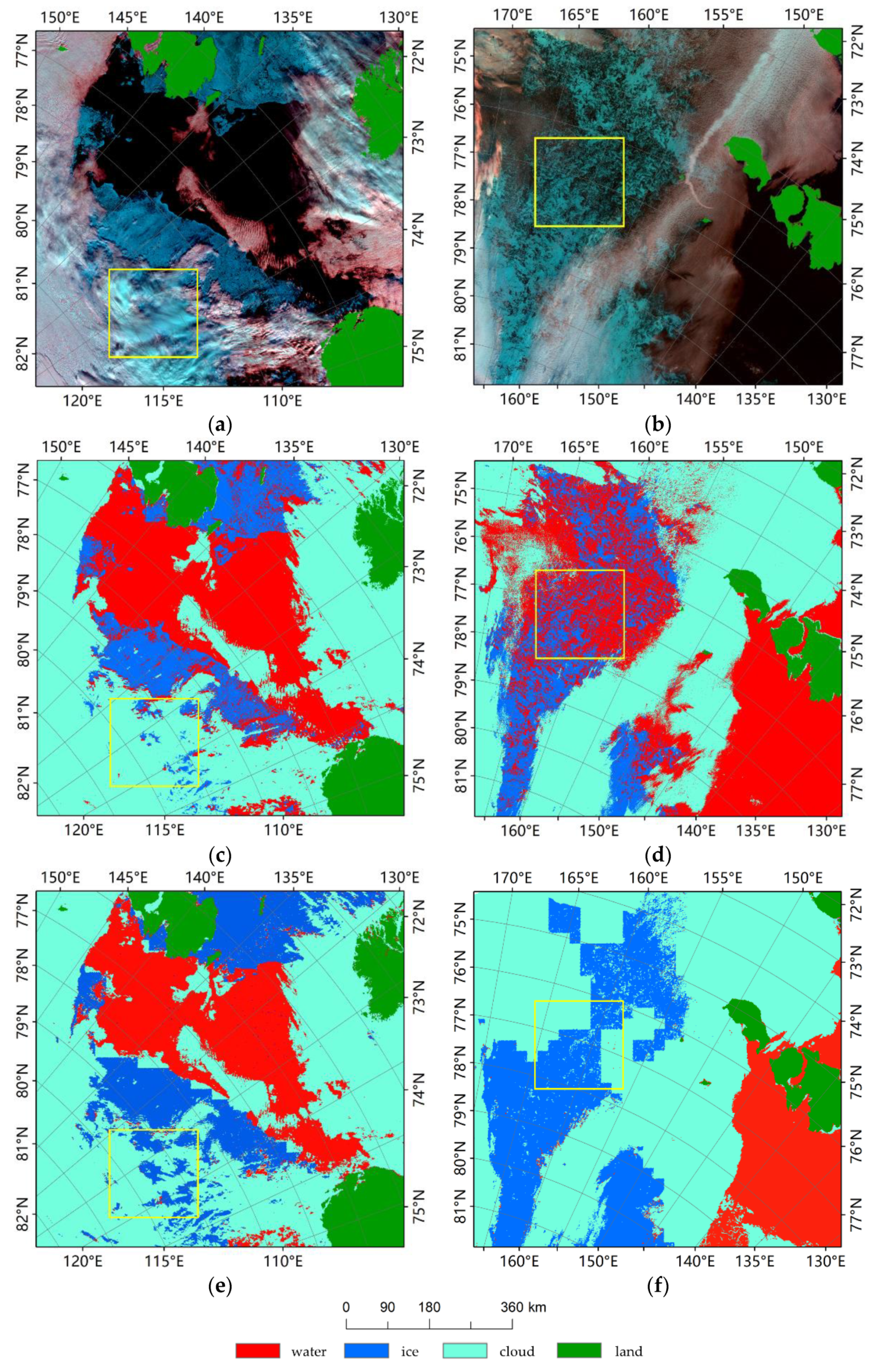
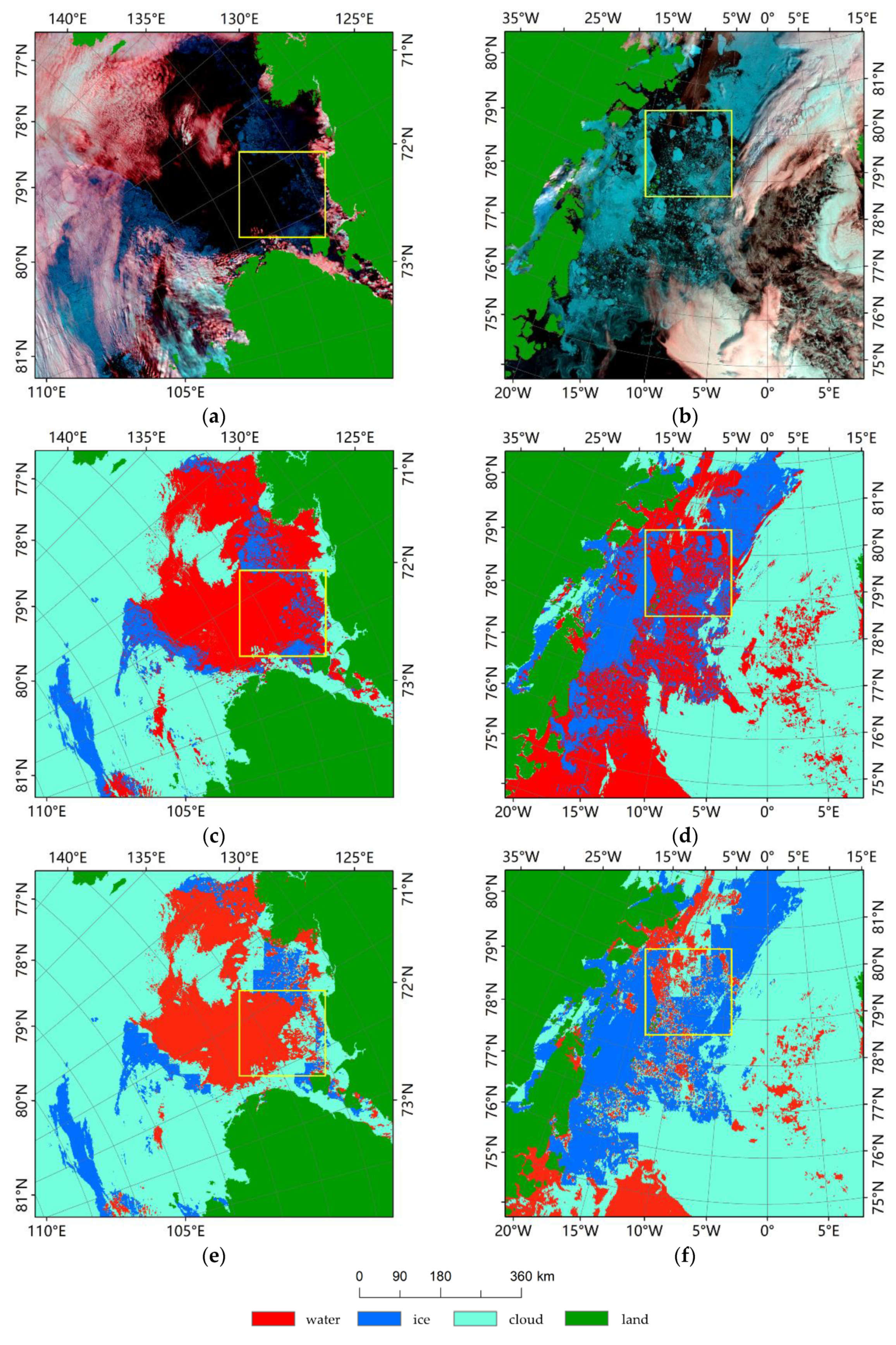
In the polar regions, the recognition accuracy of ice, cloud, and water has always been an urgent problem to be solved, especially in the sea ice areas covered by thin clouds, and ice–water mixing areas including broken ice areas and submerged ice areas, which are easily confused. In this study, several groups of representative regions were selected to show the results of the classification. In order to illustrate the effectiveness of the training sample library established in this article and the accuracy of the results, the classification results of images from different locations acquired by the two satellites at different times using the MFLFRF algorithm are compared in Figure 3 and Figure 4. They were selected from the Terra and Aqua satellites on 3 July 2018, and 3 August 2019, and contained thin ice, broken ice, and thin clouds.
It can be seen from that, compared with the MOD29 sea ice products, the results obtained by the MFLFRF algorithm can more accurately identify cloud areas, ice areas, and water areas. The recognition accuracy of the boundary regions between thin clouds, thin ice, and water is more accurate. In the blue cloud regions (displayed as blue in the bands 7, 2, and 1 combination mode) in the yellow frame in Figure 3a, the area in the MOD29 ice map is misidentified as ice by looking at Figure 3a,e. The ice map obtained by the MFLFRF algorithm can accurately identify blue clouds in this area, but some small cloud shadow areas are misidentified. For the identification of complex areas where ice and water are mixed (as shown in the yellow box in Figure 3b), the MOD29 ice map fails to identify the water areas, while the MFLFRF algorithm can accurately identify water and ice. In the water area in the yellow frame area in Figure 4a, some water areas in the MOD29 ice map were misidentified as cloud areas, while the MFLFRF algorithm accurately identified them as water areas. The MFLFRF algorithm can accurately identify the detailed information of the broken ice area in the yellow frame area in Figure 4b.

3.1.2. The Daily and Weekly Composite Ice Presence Maps

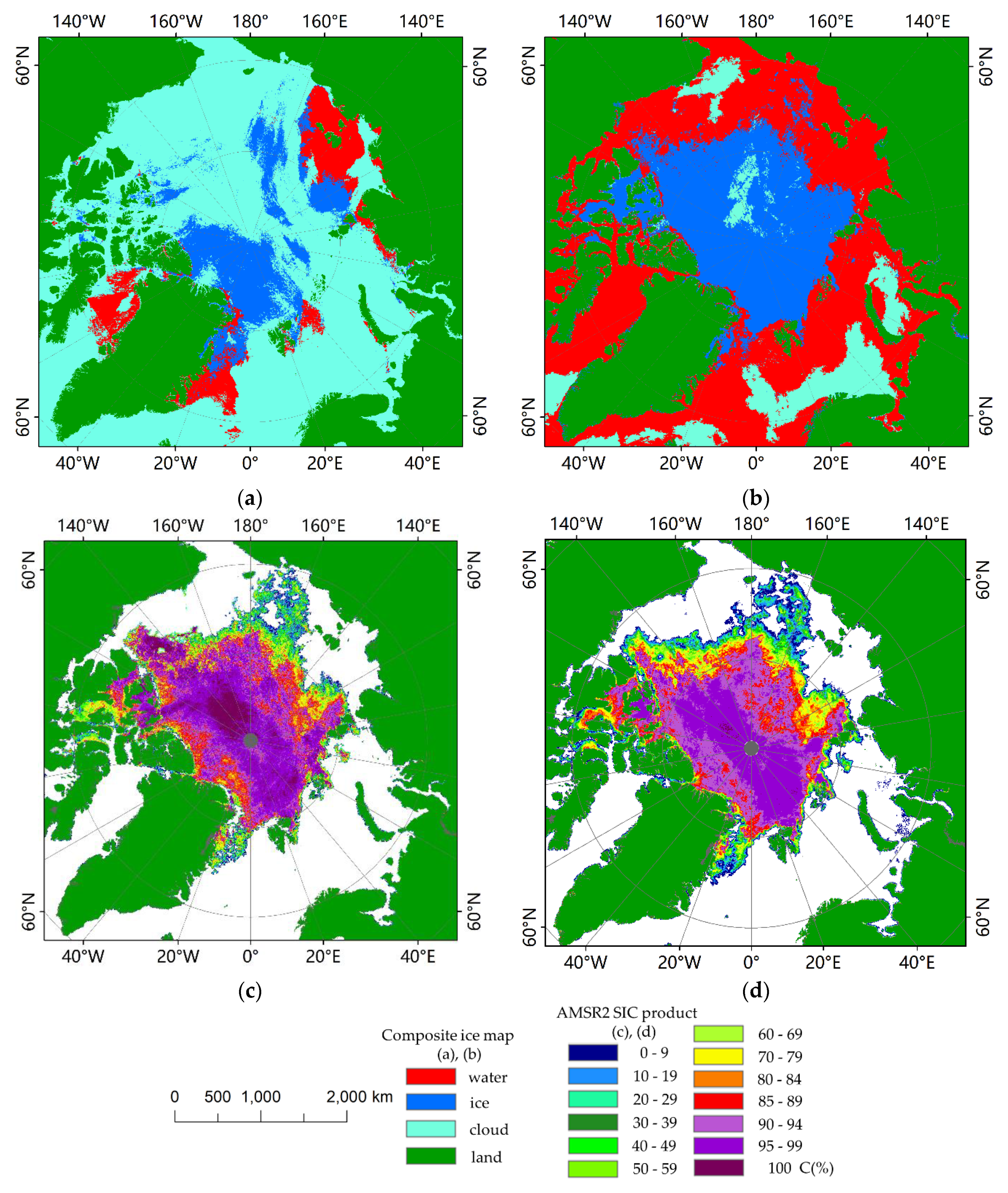
Based on the classification results of the MFLFRF algorithm, the daily and weekly composite ice presence maps were obtained using a filtering method based on cloud motion feature characteristics. Figure 5 shows the daily and weekly comparison ice maps with SIC products from AMSR2.
Due to the influence of clouds in the Arctic region, the distribution of daily clear sky areas is sparse and irregular. As shown in Figure 5a, the daily ice map is covered by clouds in most areas of the Arctic. Compared with the SIC map from AMSR2 (Figure 5c), it was found that the spatial distribution of sea ice in the daily ice map under clear sky conditions was relatively consistent with that of the SIC map. The weekly composite ice presence map (Figure 5b) and the weekly average SIC map from AMSR2 (Figure 5d) have a strong consistency in their distribution of sea ice in clear sky regions, especially in the edge regions of sea ice. Most areas in the weekly composite ice map are clear sky areas, but there are still some areas covered by clouds for seven consecutive days that show cloud areas.

3.1.3. The Weekly Fused Optical Images

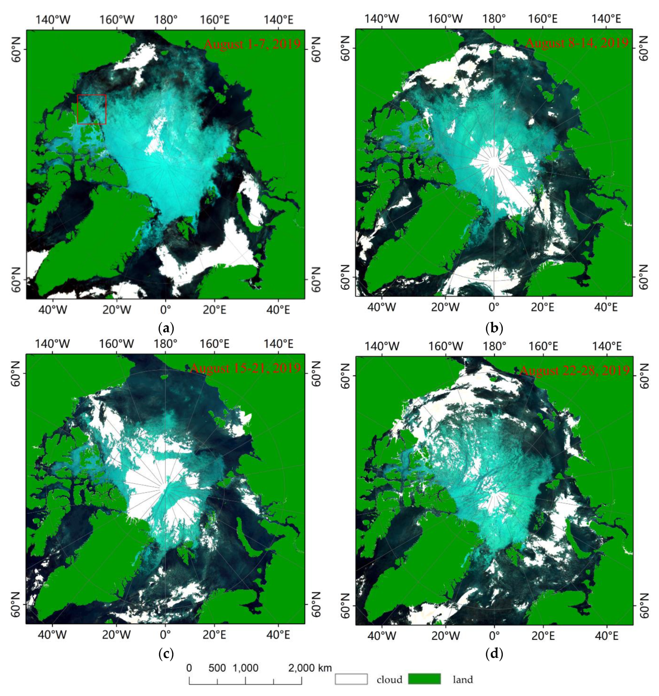
The cloud areas classified by the MFLFRF algorithm were corrected using the daily ice presence maps. According to the corrected classification results, the fused optical images were obtained by the weighted average fusion method. Figure 6 shows the weekly fusion images for four consecutive weeks from 1 to 28 August 2019.
From the weekly fusion images of the first four weeks of August 2019 (Figure 6a–d), it can be seen that the Arctic sea ice was in a melting state as a whole. On the whole, the area covered by clouds in the fusion map in the first week of August was relatively small, and the image quality was better. The areas covered by clouds in the next three weeks were more extensive, and the quality of the fusion images was affected. Comparing the weekly fused image with the average weekly SIC maps of AMSR2 in the first week of August 2019 (Figure 5d and Figure 6a), it can be clearly seen that the spatial distribution of ice in the fusion image obtained by the algorithm proposed in this study was consistent with the SIC map of AMSR2.

3.2. Accuracy of the Ice Map Products

3.2.1. Accuracy of the Single-Scene Ice Presence Maps

In order to verify the classification accuracy of the MFLFRF algorithm using fixed training samples, we randomly selected 100 images from all the images covering the Arctic region in August 2019 and September 2020, and 40 verification points were randomly selected for each image, with a total of 4000 verification points. A 6.25 km regularly spaced grid was generated by taking the verification points, and the mode of all points in the grid was taken as the category of the grid. Then, the verification points were selected randomly, with the grid as the unit. Using the false color image of bands 7, 2, and 1 combination mode with a 250 m spatial resolution, the artificial photo interpretation was performed on each verification point to obtain the true category of the feature. The thin ice at the edge of the ice area is classified as ice category, and the ice area or water area covered by thin clouds is classified as cloud category, when performing the artificial photo interpretation. The entire artificial photo interpretation process was carried out with ArcGIS software. According to the image’s texture, color, shape, and other characteristics, the verification points on the grid were interpreted one by one as ice, water, or clouds using expert judgment. The final results of the artificial photo interpretation were the combination of three independent people, and the majority voting rule was used to get the final classification results. About 30 grid points can be manually classified in one minute. The results of artificial photo interpretation were taken as the true values, and the accuracy of the classification results using the MFLFRF algorithm and the MOD29 products was evaluated, respectively. The verification results are shown in Table 3 and Table 4.
On the whole, the accuracy of the MFLFRF algorithm recognition results is much higher than that of the MOD29 products. The mapping accuracy of the results from the MFLFRF algorithm is over 96%, the accuracy rate for ice recognition is 98.49%, and the accuracy rate for cloud recognition is 98.73%. The main error source in the classification results obtained by the MFLFRF algorithm is the mislabeling of sea ice as a cloud category. This is mainly because it is easy to classify the ice covering thin clouds into ice categories during artificial photo interpretation, while the MFLFRF algorithm classifies the area into cloud categories. However, these regions are easy to be judged as ice categories during manual discrimination, which affects the accuracy of the verification results. The mapping accuracy of the MOD29 products is 86.86%, the accuracy rate of ice recognition is 79.08%, and the accuracy rate of cloud recognition is 97.45%. The main reason for the low accuracy of ice recognition in MOD29 products is that blue clouds (displayed as blue in the bands 7, 2, and 1 combination mode) are mistakenly classified as ice (as shown in the yellow box in Figure 3a). Therefore, another reason for the lower evaluation accuracy of MOD29 may be related to the spatial resolution of the products being coarser than that of the MFLFRF products. For example, the MOD29 ice map cannot identify the water area in the mixed area of ice and water in Figure 3f.

3.2.2. Accuracy of Daily and Weekly Composite Ice Presence Maps

In the accuracy verification of the daily composite ice presence maps, the number of verification points selected for the daily ice maps was not the same, because the clear sky areas of each daily ice presence maps were not equal. A set of 3000 verification points was randomly selected from the clear sky area of the daily composite ice presence maps in August 2019 and September 2020, and the daily SIC maps of AMSR2 were used as the true values to verify the synthetic products. The verification results are as shown in Table 5.
The accuracy of the weekly synthetic composite ice presence maps in the clear sky area in August 2019 and September 2020 was verified using the average weekly SIC maps of AMSR2 as the true values. There were four weekly composite ice presence maps, each of which randomly selected 100 points, with a total of 800 verification points. The verification results are shown in Table 6.
Table 5 shows that the main source of error in the daily composite ice presence maps is the misclassification of sea ice as water. Factors that may affect the accuracy of the evaluation results include the edges of deformed ice, melt ponds, and openings in the ice cover that tend to be narrow features (such as leads), which may not be detected in SIC products from AMSR2 with a spatial resolution of 6.25 km [31,53,54].
Similarly, the main source of error in the weekly composite ice presence maps shown in Table 6 is also the misclassification of sea ice as water. In addition to the different spatial resolutions of the two products, the main factor affecting the accuracy of the products may be that the edge details of the sea ice are smoothed out when averaging the daily SIC products from AMSR2. The weekly ice presence maps are the results of synthesis, and the two products may have errors on some ice edges.

3.2.3. Accuracy of Weekly Fused Optical Images

Since the weekly fused optical images are based on the classification results of the pre-processed image sets for clear sky fusion, it is difficult to quantitatively verify these composite images. In this study, the products are compared with the existing enlarged drawings of SIC products from AMSR2 in Figure 7. The sea ice spatial distribution of the weekly fused optical images is consistent with that of the SIC products, but they are easily covered by clouds and cannot map the entire Arctic region. The weekly fusion images can fully retain the detailed information of sea ice distribution, especially the texture details of ice in the marginal ice zone.

4. Discussion

Previous work has mostly used passive microwave data with a coarse spatial resolution to monitor polar sea ice [15,17], and radar data with a higher spatial resolution to monitor sea ice conditions in local areas [28,29]. Because optical data are affected by clouds and fog, and because it is difficult to distinguish between them and ice and snow, they are rarely used in large-scale and long-term sea ice monitoring and analysis of polar regions. In this study, we used MODIS data to realize polar ice map products and fusion products with a higher spatial resolution.
The improvement in spatial resolution can help the products to detect smaller features. However, cloud cover is the most restrictive obstacle to using optical data to map sea ice [31]. In traditional ice map products, there are some areas where clouds are mislabeled as ice. In this study, using the method of multi-feature combination, the prevalence of the phenomenon where clouds are incorrectly marked as ice in ice maps obtained by the RF machine learning classification method is lower than that of the MOD29 product, and the overall classification accuracy is higher.
Using the false color combination of MODIS reflectance bands 7, 2, and 1, ice and cloud types can be distinguished more accurately. The NDSII-2 index can highlight most of the ice and snow features, so adding the NDSII-2 index feature can greatly improve the classification accuracy. The blue high clouds and cold clouds composed of small ice crystals are difficult to distinguish from sea ice, which is also a problem in traditional methods of monitoring sea ice [31]. In this study, based on the texture difference between blue clouds and sea ice, RELBP texture features were added when using the MFLFRF classification algorithm to distinguish blue clouds and sea ice.
Although the MFLFRF classification algorithm has greatly improved the recognition accuracy of ice and clouds, there are still some areas with cloud shadows and blue clouds that are misidentified as ice. According to the movement characteristics of clouds, when compositing ice images the number of occurrences of non-cloud categories in the same pixel in all classified images in a day can be used to effectively remove this type of classification error. Combining the classification results of all the images covering the Arctic region for seven consecutive days, it was possible to obtain a clear sky ice map for most of the areas, but there were still some areas covered by clouds for seven consecutive days.

5. Conclusions

The fully automatic ice map generation model proposed by this research uses the highest possible spatial resolution of MODIS-Terra and Aqua satellite reflectance data and can provide a sea ice presence map with 250-meter spatial resolution. This model greatly improves the recognition accuracy of ice and clouds, can realize the production of near real-time ice maps, and can be used in many scientific and practical applications in the future.
This model uses a machine learning method that integrates multiple features to identify ice and clouds. Compared with traditional ice map products, the accuracy is greatly improved, and its accuracy reaches more than 98%. On the basis of high-precision classification, daily and weekly synthetic ice presence maps and weekly clear sky images are realized. The polar regions are extremely affected by clouds. Although most areas of the weekly synthetic ice map are clear, there are still a few areas covered by clouds. In the future, the composite algorithm will be further improved to replace these cloud-covered areas with clear sky images so as to achieve daily or weekly cloudless clear sky images.

Author Contributions

L.J. and F.C. conceived and designed the experiments, processed the data, and wrote the manuscript; L.J. and Y.M. processed and analyzed the data; W.Y. and J.L. discussed the result; W.Y. and E.S. investigated the results and revised the manuscript; Y.M. and L.J. investigated the results, revised the manuscript, and supervised this study. All authors have read and agreed to the published version of the manuscript.

Funding

This research was supported by the International Partnership Program of Chinese Academy of Sciences (NO. 131211KYSB20170041), the National Key Research and Development Program of China (No. 2017YFE0111700), and the Strategic Priority Research Program of the Chinese Academy of Sciences (No. XDA19070201).

Acknowledgments

We greatly thank the editor and four anonymous reviewers for their constructive comments, which helped us to improve the manuscript.

Conflicts of Interest

The authors declare no conflict of interest.

References

  1. Pörtner, H.-O.; Roberts, D.C.; Masson-Delmotte, V.; Zhai, P.; Tignor, M.; Poloczanska, E.; Mintenbeck, K.; Alegría, A.; Nicolai, M.; Okem, A. IPCC, 2019: IPCC Special Report on the Ocean and Cryosphere in a Changing Climate. p. 765. Available online: https://www.ipcc.ch/srocc/ (accessed on 12 November 2019).
  2. Suddenly in Second Place. Available online: http://nsidc.org/arcticseaicenews/2020/10/lingering-seashore-days/ (accessed on 5 October 2020).
  3. Maslanik, J.; Dunn, J. On the role of sea-ice transport in modifying arctic responses to global climate change. Ann. Glaciol. 1996, 25, 102–106. [Google Scholar] [CrossRef] [Green Version]
  4. Diebold, F.X.; Rudebusch, G.D. Probability Assessments of an Ice-Free Arctic: Comparing Statistical and Climate Model Projections. Working Pap. Ser. 2020. [Google Scholar] [CrossRef] [Green Version]
  5. Vickers, H.; Karlsen, S.R.; Malnes, E. A 20-Year MODIS-Based Snow Cover Dataset for Svalbard and Its Link to Phenological Timing and Sea Ice Variability. Remote. Sens. 2020, 12, 1123. [Google Scholar] [CrossRef] [Green Version]
  6. Dupont, N.; Durant, J.M.; Langangen, Ø.; Gjøsæter, H.; Stige, L.C. Sea ice, temperature, and prey effects on annual variations in mean lengths of a key Arctic fish, Boreogadus saida, in the Barents Sea. ICES J. Mar. Sci. 2020, 77, 1796–1805. [Google Scholar] [CrossRef]
  7. Song, C.; Zhang, Y.; Xu, Z.; Hao, Z.; Wang, X. Route Selection of the Arctic Northwest Passage Based on Hesitant Fuzzy Decision Field Theory. IEEE Access 2019, 7, 19979–19989. [Google Scholar] [CrossRef]
  8. Wang, Q.; Lu, P.; Zu, Y.; Li, Z.; Leppäranta, M.; Zhang, G. Comparison of Passive Microwave Data with Shipborne Photographic Observations of Summer Sea Ice Concentration along an Arctic Cruise Path. Remote. Sens. 2019, 11, 2009. [Google Scholar] [CrossRef] [Green Version]
  9. Haas, C.; Howell, S.E.L. Ice thickness in the Northwest Passage. Geophys. Res. Lett. 2015, 42, 7673–7680. [Google Scholar] [CrossRef]
  10. Su, J.; Xu, N.; Zhao, J.; Li, X. Features of Northwest Passage Sea Ice’s Distribution and Variation under Arctic Rapidly Warming Condition. Chin. J. Polar Res. 2010, 22, 104–124. [Google Scholar] [CrossRef]
  11. Cong, X. Potential Influence of the Northwest Passage on Global Economics and China’s Countermeasures: Based on Global Multi-Regional CGE Model. World Econ. Polit. 2017, 2, 106–129. [Google Scholar]
  12. Ivanova, N.; Pedersen, L.T.; Tonboe, R.; Kern, S.; Heygster, G.; Lavergne, T.; Sorensen, A.C.; Saldo, R.; Dybkjaer, G.; Brucker, L.; et al. Inter-comparison and evaluation of sea ice algorithms: Towards further identification of challenges and optimal approach using passive microwave observations. Cryosphere 2015, 9, 1797–1817. [Google Scholar] [CrossRef] [Green Version]
  13. Markus, T.; Cavalieri, D. An enhancement of the NASA Team sea ice algorithm. IEEE Trans. Geosci. Remote. Sens. 2002, 38, 1387–1398. [Google Scholar] [CrossRef] [Green Version]
  14. Shokr, M.; Lambe, A.; Agnew, T. A New Algorithm (ECICE) to Estimate Ice Concentration from Remote Sensing Observations: An Application to 85-GHz Passive Microwave Data. IEEE Trans. Geosci. Remote. Sens. 2008, 46, 4104–4121. [Google Scholar] [CrossRef]
  15. Spreen, G.; Kaleschke, L.; Heygster, G. Sea ice remote sensing using AMSR-E 89-GHz channels. J. Geophys. Res. Space Phys. 2008, 113. [Google Scholar] [CrossRef] [Green Version]
  16. Meier, W.; Stewart, J.S. Assessing the Potential of Enhanced Resolution Gridded Passive Microwave Brightness Temperatures for Retrieval of Sea Ice Parameters. Remote. Sens. 2020, 12, 2552. [Google Scholar] [CrossRef]
  17. Cavalieri, D.J.; Parkinson, C.L.; Gloersen, P.; Zwally, H.J. Arctic and Antarctic Sea Ice Concentrations from Multichannel Passive-Microwave Satellite Data Sets: October 1978–September 1995: User’s Guide. NASA Tech. Memo. 1997, 17, 104647. [Google Scholar]
  18. Alexander, B.; Lars, K.; Stefan, K.J.R.S. Investigating High-Resolution AMSR2 Sea Ice Concentrations during the February 2013 Fracture Event in the Beaufort Sea. Remote Sens. 2014, 6, 3841–3856. [Google Scholar]
  19. Comiso, J.C.; Meier, W.; Markus, T. Annomalies and Trends in the Sea Ice Cover from 40 years of Passive Microwave Data. In Proceedings of the AGU Fall Meeting Abstracts, Washington, DC, USA, 10–14 December 2018. [Google Scholar]
  20. Eastwood, S. Sea Ice Product User’s Manual OSI-401-a, OSI402-a, OSI-403-a; Version 3.11; EUMETSAT: Darmstadt, Germany, 2014. [Google Scholar]
  21. Zhao, J.; Zhou, X.; Sun, X.; Cheng, J.; Bo, H.U.; Chunhua, L.I.; Press, C.O. The inter comparison and assessment of satellite sea-ice concentration datasets from the arctic. Remote Sens. 2017, 21, 351–364. [Google Scholar]
  22. Scheuchl, B.; Caves, R.; Cumming, I.; Staples, G. Automated sea ice classification using spaceborne polarimetric SAR data. In Proceedings of the IEEE International Geoscience and Remote Sensing Symposium, Sydney, Australia, 9–13 July 2001. IEEE Cat. No.01CH37217. [Google Scholar]
  23. Soh, L.-K.; Tsatsoulis, C.; Gineris, D.; Bertoia, C. ARKTOS: An Intelligent System for SAR Sea Ice Image Classification. IEEE Trans. Geosci. Remote. Sens. 2004, 42, 229–248. [Google Scholar] [CrossRef] [Green Version]
  24. Yu, Q.; Clausi, D.A. SAR Sea-Ice Image Analysis Based on Iterative Region Growing Using Semantics. IEEE Trans. Geosci. Remote. Sens. 2007, 45, 3919–3931. [Google Scholar] [CrossRef]
  25. Chen, S.; Shokr, M.; Li, X.; Ye, Y.; Zhang, Z.; Hui, F.; Cheng, X. MYI Floes Identification Based on the Texture and Shape Feature from Dual-Polarized Sentinel-1 Imagery. Remote. Sens. 2020, 12, 3221. [Google Scholar] [CrossRef]
  26. Kruk, R.; Fuller, M.C.; Komarov, A.S.; Isleifson, D.; Jeffrey, I. Proof of Concept for Sea Ice Stage of Development Classification Using Deep Learning. Remote. Sens. 2020, 12, 2486. [Google Scholar] [CrossRef]
  27. Aulicino, G.; Wadhams, P.; Parmiggiani, F. SAR Pancake Ice Thickness Retrieval in the Terra Nova Bay (Antarctica) during the PIPERS Expedition in Winter 2017. Remote. Sens. 2019, 11, 2510. [Google Scholar] [CrossRef] [Green Version]
  28. Boulze, H.; Korosov, A.; Brajard, J. Classification of Sea Ice Types in Sentinel-1 SAR Data Using Convolutional Neural Networks. Remote. Sens. 2020, 12, 2165. [Google Scholar] [CrossRef]
  29. Ding, F.; Shen, H.; Perrie, W.; He, Y. Is Radar Phase Information Useful for Sea Ice Detection in the Marginal Ice Zone? Remote. Sens. 2020, 12, 1847. [Google Scholar] [CrossRef]
  30. Shokr, M.; Sinha, N. Sea Ice: Physics and Remote Sensing; John Wiley & Sons: Hoboken, NJ, USA, 2015. [Google Scholar]
  31. Gignac, C.; Bernier, M.; Chokmani, K.; Poulin, J. IceMap250—Automatic 250 m Sea Ice Extent Mapping Using MODIS Data. Remote. Sens. 2017, 9, 70. [Google Scholar] [CrossRef] [Green Version]
  32. Drüe, C. High-resolution maps of the sea-ice concentration from MODIS satellite data. Geophys. Res. Lett. 2004, 312, 183–213. [Google Scholar] [CrossRef]
  33. Choi, H.; Bindschadler, R. Cloud detection in Landsat imagery of ice sheets using shadow matching technique and automatic normalized difference snow index threshold value decision. Remote Sens. Environ. 2004, 91, 237–242. [Google Scholar] [CrossRef]
  34. Xiao, X.; Shen, Z.; Qin, X. Assessing the potential of vegetation sensor data for mapping snow and ice cover: A Normalized Difference Snow and Ice Index. Int. J. Remote Sens. 2001, 22, 2479–2487. [Google Scholar] [CrossRef]
  35. Keshri, A.K.; Shukla, A.; Gupta, R.P. ASTER ratio indices for supraglacial terrain mapping. Int. J. Remote. Sens. 2008, 30, 519–524. [Google Scholar] [CrossRef]
  36. Zhan, Y.; Wang, J.; Shi, J.; Cheng, G.; Yao, L.; Sun, W. Distinguishing Cloud and Snow in Satellite Images via Deep Convolutional Network. IEEE Geosci. Remote. Sens. Lett. 2017, 14, 1785–1789. [Google Scholar] [CrossRef]
  37. Varshney, D.; Gupta, P.K.; Persello, C.; Nikam, B.R. Snow and Cloud Discrimination using Convolutional Neural Networks. ISPRS Ann. Photogramm. Remote Sens. Spat. Inf. Sci. 2018, 4, 59–63. [Google Scholar] [CrossRef] [Green Version]
  38. Ghasemian, N.; Akhoondzadeh, M. Introducing two Random Forest based methods for cloud detection in remote sensing images. Adv. Space Res. 2018, 62, 288–303. [Google Scholar] [CrossRef]
  39. Hall, D.K.; Riggs, G. MODIS/Terra Sea Ice Extent 5-Min L2 Swath 1 km; Version 6; NASA National Snow and Ice Data Center Distributed Active Archive Center: Boulder, CO, USA, 2015. [Google Scholar] [CrossRef]
  40. Chan, M.A.; Comiso, J.C. Arctic Cloud Characteristics as Derived from MODIS, CALIPSO, and CloudSat. J. Clim. 2013, 26, 3285–3306. [Google Scholar] [CrossRef]
  41. Wolfe, R.; Roy, D.; Vermote, E. MODIS land data storage, gridding, and compositing methodology: Level 2 grid. IEEE Trans. Geosci. Remote. Sens. 1998, 36, 1324–1338. [Google Scholar] [CrossRef] [Green Version]
  42. Running, S.W.; Justice, C.; Salomonson, V.; Hall, D.; Barker, J.; Kaufmann, Y.J.; Strahler, A.H.; Huete, A.R.; Muller, J.; Vanderbilt, V.; et al. Terrestrial remote sensing science and algorithms planned for EOS/MODIS. Int. J. Remote. Sens. 1994, 15, 3587–3620. [Google Scholar] [CrossRef]
  43. Zhou, J.; Zhou, R.; Li, S.; Ding, K. Research of MODIS L1B-level Data Radiometric Correction and Solar Zenith Correction. J. Northeast For. Univ. 2010, 30, 77–81. [Google Scholar]
  44. Bishop, M.P.; Bjornsson, H.; Haeberli, W.; Oerlemans, J.; Shroder, J.F.; Tranter, M.; Singh, V.P.; Haritashya, U.K. Encyclopedia of Snow, Ice and Glaciers; Springer: Berlin, Germany, 2011. [Google Scholar] [CrossRef]
  45. Dozier, J. Spectral signature of alpine snow cover from the landsat thematic mapper. Remote. Sens. Environ. 1989, 28, 9–22. [Google Scholar] [CrossRef]
  46. Shao, Z.; Deng, J.; Wang, L.; Fan, Y.; Sumari, N.S.; Cheng, Q. Fuzzy AutoEncode Based Cloud Detection for Remote Sensing Imagery. Remote. Sens. 2017, 9, 311. [Google Scholar] [CrossRef] [Green Version]
  47. Ojala, T.; Pietikainen, M.; Maenpaa, T. Multiresolution gray-scale and rotation invariant texture classification with local binary patterns. IEEE Trans. Pattern Anal. Mach. Intell. 2002, 24, 971–987. [Google Scholar] [CrossRef]
  48. Liu, L.; Lao, S.; Fieguth, P.W.; Guo, Y.; Wang, X.; Pietikainen, M. Median Robust Extended Local Binary Pattern for Texture Classification. IEEE Trans. Image Process. 2016, 25, 1368–1381. [Google Scholar] [CrossRef]
  49. Guan, H.; Li, J.; Chapman, M.; Deng, F.; Ji, Z.; Yang, X. Integration of orthoimagery and lidar data for object-based urban thematic mapping using random forests. Int. J. Remote. Sens. 2013, 34, 5166–5186. [Google Scholar] [CrossRef]
  50. Rodriguez-Galiano, V.; Ghimire, B.; Rogan, J.; Chicaolmo, M.; Rigol-Sanchez, J. An assessment of the effectiveness of a random forest classifier for land-cover classification. ISPRS J. Photogramm. Remote. Sens. 2012, 67, 93–104. [Google Scholar] [CrossRef]
  51. Du, P.; Samat, A.; Waske, B.; Liu, S.; Li, Z. Random Forest and Rotation Forest for fully polarized SAR image classification using polarimetric and spatial features. ISPRS J. Photogramm. Remote. Sens. 2015, 105, 38–53. [Google Scholar] [CrossRef]
  52. Topouzelis, K.; Psyllos, A. Oil spill feature selection and classification using decision tree forest on SAR image data. ISPRS J. Photogramm. Remote. Sens. 2012, 68, 135–143. [Google Scholar] [CrossRef]
  53. Lee, S.H.; Stockwell, D.A.; Joo, H.-M.; Son, Y.B.; Kang, C.-K.; Whitledge, T.E. Phytoplankton production from melting ponds on Arctic sea ice. J. Geophys. Res. Space Phys. 2012, 117, 4030. [Google Scholar] [CrossRef]
  54. Perovich, D.K.; Richter-Menge, J.A. Surface characteristics of lead ice. J. Geophys. Res. Space Phys. 1994, 99, 16341–16350. [Google Scholar] [CrossRef]
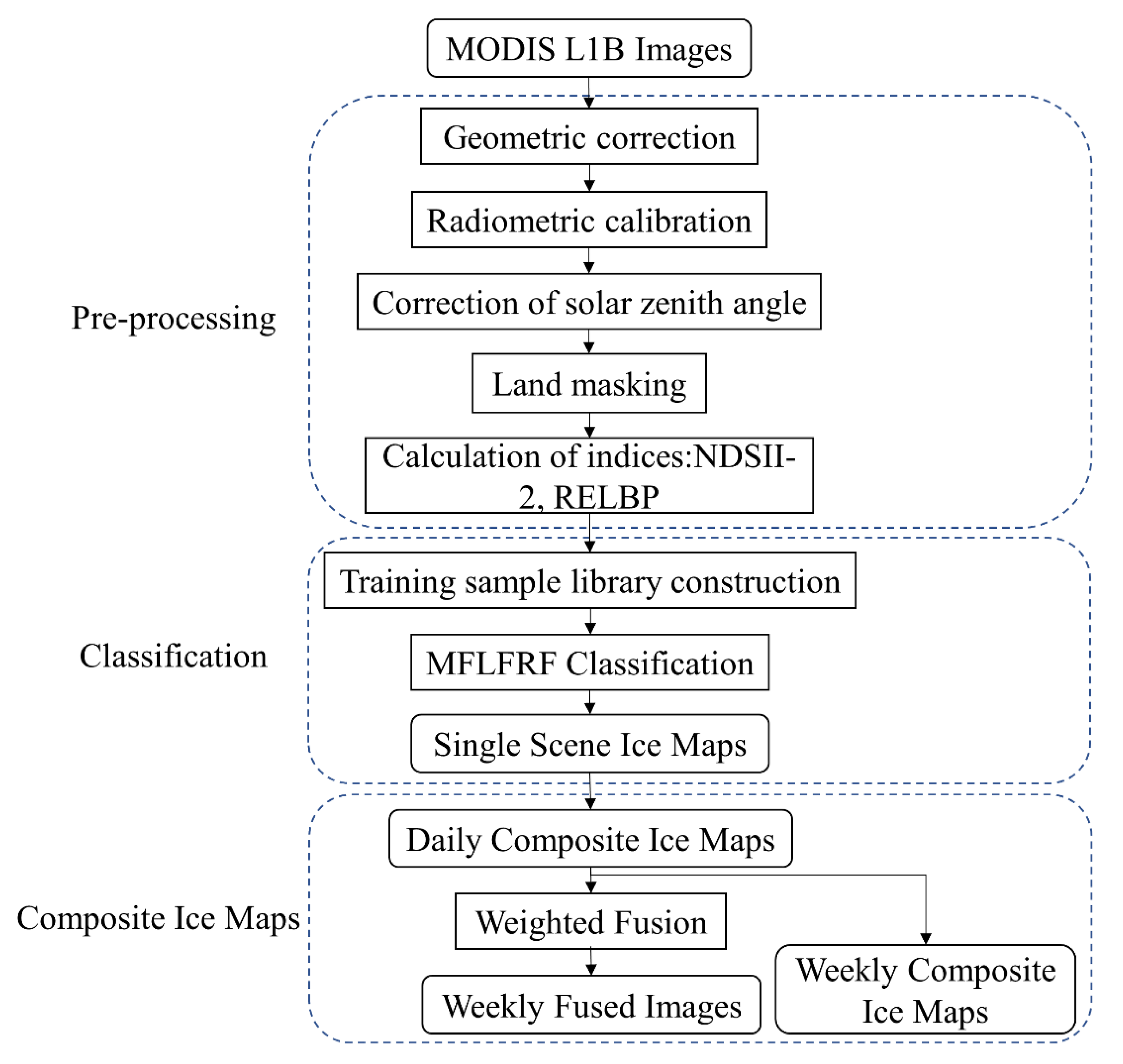
Figure 1. Representation of the methodological framework used in this study.
Remotesensing 13 00550 g001
Figure 2. Representation of the methodological framework used in Section 2.2.3. Here, N represents the number of occurrences of non-cloud categories for each pixel, T1 is the threshold of the number of ice occurrences for each pixel, and T2 is the threshold of the number of occurrences of water for each pixel.
Remotesensing 13 00550 g002
Figure 3. Process illustration using Terra satellite imagery as an example. (a) and (b) are both false colors images of the combination of bands 7, 2, and 1, and the acquisition times are 3 July 2018, and 3 August 2019, respectively; (c) and (d) are the classification results of (a) and (b) images using the MFLFRF algorithm; (e) and (f) are the corresponding MOD29 sea ice products of (a) and (b) images, respectively.
Remotesensing 13 00550 g003
Figure 4. Process illustration using Aqua satellite imagery as an example. (a) and (b) are both false color images of the combination of bands 7, 2, and 1, and the acquisition times are 3 July 2018, and 3 August 2019, respectively; (c) and (d) are the classification results of (a) and (b) images using the MFLFRF algorithm; (e) and (f) are the corresponding MOD29 sea ice products of (a) and (b) images, respectively.
Remotesensing 13 00550 g004
Figure 5. Comparison of daily and weekly composite ice presence maps and SIC maps from AMSR2. (a) is the daily synthetic ice map from the Terra satellite on 1 August 2019. (b) is the weekly synthetic ice map from the Terra and Aqua satellites on 1–7 August 2019. (c) is the daily SIC map from AMSR2 on 1 August 2019. (d) is the SIC seven-day average map from AMSR2 on 1–7 August 2019.
Remotesensing 13 00550 g005
Figure 6. The weekly fusion images for four consecutive weeks from 1 to 28 August 2019. (a) to (d) all both false color images of the combination of bands 7, 2, and 1. The red frame in Figure 6a is shown in detail in Figure 7a.
Remotesensing 13 00550 g006
Figure 7. Comparison of the weekly fusion image and the SIC seven-day average from AMSR2. (a) is an enlarged image of the red rectangular area of Figure 6a, and (b) is the SIC from AMSR2 in the red rectangular area of Figure 6a.
Remotesensing 13 00550 g007
Table 1. Spatial and spectral characteristics of MODIS reflection bands 1–7.
Band NumberSpatial Resolution (m)Bandwidth (μm)Part of Spectrum
12500.620–0.670VIR (red)
22500.841–0.876NIR
35000.459–0.479VIR (blue)
45000.545–0.565VIR (green)
55001.230–1.250NIR
65001.628–1.652SWIR
75002.105–2.155SWIR
Table 2. Details of the training sample library. Ice, water, cloud 1, cloud 2, and cloud 3.
Sample CategoryIceWaterCloud
Cloud 1Cloud 2Cloud 3
Total Pixels14,16213,94410,05711,29210,343
Table 3. Accuracy of the classification results using the MFLFRF algorithm.
Ground Truth
WaterIceCloudTotalCommission Error
MFLFRF MapWater489724981.81%
Ice039263981.51%
Cloud039306531041.27%
Total48943830734000N/A
Omission Error0.00%10.50%0.26%N/A
Overall Accuracy98.65%
Table 4. Accuracy of the MOD29 products.
Ground Truth
WaterIceCloudTotalCommission Error
MOD29 MapWater4419164665.36%
Ice213787947820.92%
Cloud2751297830562.55%
Total48943830734000N/A
Omission Error10.88%13.70%3.09%N/A
Overall Accuracy94.93%
Table 5. Accuracy of the daily composite ice presence maps.
AMSR2 Sea Ice Maps
WaterIceTotalCommission Error
MFLFRF MapWater894419354.39%
Ice3206220650.15%
Total89721033000N/A
Omission Error0.33%1.95%N/A
Overall Accuracy98.53%
Table 6. Accuracy of the weekly composite ice presence maps.
AMSR2 Sea Ice Maps
WaterIceTotalCommission Error
MFLFRF MapWater23992483.63%
Ice2 5505520.36%
Total241559800N/A
Omission Error0.83%1.64%N/A
Overall Accuracy98.60%
Publisher’s Note: MDPI stays neutral with regard to jurisdictional claims in published maps and institutional affiliations.