1. Introduction
Accurate and reliable measurements of atmospheric water vapor’s vertical profile are essential for characterizing and understanding meteorological and climate processes. For instance, these observations are routinely assimilated in operational numerical weather prediction (NWP) models to produce accurate weather forecasts. Water vapor drives atmospheric dynamics, affects atmospheric chemistry, and has a significant impact on radiative transfer [
1,
2,
3]. Measurements are particularly crucial within the planetary boundary layer (PBL), where the variability of humidity is not adequately observed and water cycles remain poorly understood [
4,
5].
Currently, operational water vapor profile measurements over land are dominated by global radiosonde (RS) observations, which occur only twice a day at most sites. Though they are an established and relatively accurate method, there exists a demonstrated need for higher-temporal resolution observations. While several commercially available technologies such as microwave radiometers and atmospheric emitted radiance interferometers address this need, lidar observations are typically at higher resolution (temporally and vertically), continuous, and relatively cost-effective in comparison. Automated lidars designed for operational use exhibit several other advantages over RSs in particular, including their ability to conduct measurements in urban areas and during high surface winds (when RSs cannot be launched), ease to deploy (no infrastructure required), lack of measurement drift, and minimal operating cost.
The two primary lidar techniques for water vapor profiling are differential absorption lidar (DIAL) and Raman lidar. Raman lidars make use of weak inelastic scattering to determine the water vapor mixing ratio (WVMR) [
6,
7], whereas DIAL systems measure the difference in absorption between two laser wavelengths centered on and off water vapor absorption lines [
8]. Raman lidars are a mature technology that have been used for measurements of several atmospheric gases such as water vapor, ozone, carbon dioxide, and various aerosol properties [
7,
9,
10,
11,
12]. DIAL technology was accelerated during the NASA Langley DIAL program [
13] and it has also been used to measure aerosol properties and several trace gases, including water vapor [
14,
15,
16,
17,
18,
19,
20,
21].
Compared to water vapor Raman lidars, water vapor DIAL systems typically utilize smaller telescopes and, since they provide an absolute measurement of the water vapor number density, they do not require an external instrument (e.g., RS) for calibration. A DIAL’s smaller size, lower cost, and independent calibration significantly reduces a typical DIAL’s operating complexity, maintenance, size, and overall costs, making them well-suited for operational deployment in a large network. While both techniques have their challenges, the most notable disadvantages for most DIAL systems is their decreased vertical range (e.g., within the boundary layer) compared to Raman lidars, their requirement of a more stable laser source, uncertainties that arise in their WVMR retrieval algorithm due to absorption by other gases, scattering differential by aerosols, and complex analysis routines to solve the DIAL equation. Comprehensive reviews comparing the DIAL and Raman methods are provided in References [
5,
22].
In summer 2018, Environment and Climate Change Canada (ECCC) acquired a new broadband DIAL system developed by Vaisala for operational use as a stand-alone system or as part of a larger network. The DIAL demonstrated excellent performance in a summer-time urban environment during the Toronto water vapor lidar inter-comparison campaign [
23]. Its earlier prototype version also underwent evaluations in the Southern Great Plains, Germany, Finland, and Hong Kong [
24,
25,
26]. These evaluations, however, consisted of shorter (couple of months) campaigns. This new pre-production DIAL system has never undergone an evaluation over a long (multi-season) timespan, and neither the pre-production nor the earlier prototype DIAL system have been evaluated in the Arctic. The Arctic provides extreme operational conditions to assess the DIAL’s performance in a dry environment (<1 g/kg during non-summer months) with a more limited backscatter signal (due to decreased aerosols and lower PBL heights). At the same time, the Arctic water vapor budget is not well-constrained due to the lack of available measurements [
3]. A network of these DIAL systems has the potential to fill this crucial gap.
This study presents a detailed evaluation of the new pre-production Vaisala DIAL system currently operating at the Canadian Arctic Weather Science (CAWS) Iqaluit supersite (63.74°N, 68.51°W) [
27] during the World Meteorological Organization’s (WMO) Year of Polar Prediction (YOPP) project (core phase: mid-2017 to mid-2019) [
28,
29]. Comparisons between the new pre-production DIAL system and RS observations were conducted over almost one year of continuous observations (7 September 2018 to 22 August 2019), and Raman lidar comparisons were conducted over six months (7 September 2018 to 27 February 2019). Comparisons between the DIAL and the ECCC NWP models were performed over the same time period to evaluate the models’ performance at high resolution.
Section 2 describes the Iqaluit supersite, the instrumentation, and the ECCC NWP models.
Section 3 provides results on the comparisons between the DIAL, Raman, and RS observations at Iqaluit, an investigation of the DIAL’s observed bias, and a verification case study using ECCC NWP models during YOPP. A discussion of the results is provided in
Section 4. Conclusions and future work are provided in
Section 5.
2. Materials and Methods
2.1. The Iqaluit Supersite and the Year of Polar Prediction (YOPP)
The ECCC Iqaluit supersite (63.74°N, 68.51°W), located in the Arctic tundra, is ~200 m from the shoreline of Frobisher Bay, ~200 m from the Iqaluit airport runway, and several kilometers south-west of ~300 m-high hills (
Figure 1). The site was a designated supersite for the WMO YOPP project. It has been equipped with a suite of co-located remote-sensing and in-situ instruments for meteorological observations since 2015 [
28,
29]. With the enhanced meteorological observations conducted at the site, international NWP modeling centers, including ECCC, provided model output data at the model time-step in a 7 × 7 grid centered on Iqaluit and other YOPP-designated supersites during the YOPP (
https://yopp.met.no/node/54 (accessed on 13 November 2020)). This enabled enhanced model verification, inter-comparisons, and process studies to investigate difficulties with NWP model representations of the structure and physical processes within the Arctic PBL.
2.2. Vaisala Differential Absorption Lidar (DIAL)
The Vaisala pre-production broadband DIAL system provides fully automated and continuous (24 h) observations of the attenuated backscatter (every minute) and WVMR (20 min running average) vertical profile within the PBL (or up to a thick cloud base) during all weather conditions (during heavy precipitation, its range is severely limited). Despite the DIAL’s limited vertical range, most atmospheric water vapor is distributed near the surface within the PBL and hence is measureable by the DIAL. No operator is required, except for only basic, routine (yearly) maintenance (e.g., cleaning the optical windows and replacing the external USB hard drive).
The newly developed pre-production DIAL system was installed at the Iqaluit supersite on 6 September 2018 (
Figure 2, left) after undergoing a preliminary evaluation in Toronto [
23]. A second pre-production model was acquired by Deutscher Wetterdienst (DWD) and deployed to Germany, where it is undergoing its own independent assessment and field campaign. With the exception of intermittent power outages at the site, the DIAL experienced no downtime during the study period.
To measure the WVMR, two vertically pointing eye-safe (class 1M) pulsed diode lasers contained within a Vaisala CL-series ceilometer-type telescope [
24,
30] transmit and receive two wavelengths centered on (911.0 nm) and off (910.6 nm) strongly absorbing water vapor lines. Laboratory measurements of the near- and far-field laser spectral widths, required as inputs to the WVMR retrieval algorithm, were conducted using an optical spectrum analyzer. The WVMR as a function of height is then retrieved using an inversion method to solve the broadband DIAL equation, as shown in Reference [
26]. The WVMR from the near- (50 to 400 m) and far-field (300 to 3000 m) units are merged between 300 and 400 m using a linearly increasing weighting function.
The standard deviation of the water vapor profiles and the online-to-offline signal ratio over the 20 min averaging period is used to determine the WVMR uncertainty and maximum effective range, respectively. See Reference [
26] for further details on the instrument’s technical design, WVMR retrieval algorithm, and quality control. Only data above 90 m above ground level (AGL) and below its maximum effective range were used in this study. Additional specifications are provided in
Table 1.
2.3. Canadian Autonomous Arctic Aerosol Lidar (CAAAL)
The Canadian Autonomous Arctic Aerosol Lidar (CAAAL) was installed at Iqaluit in November 2016 (
Figure 2, right) [
31,
32]. It conducts automated continuous measurements (except during precipitation) of the vertical structure of particulate matter up to 15 km AGL. The lidar, housed in a trailer, was designed and built by ECCC and upgraded with a new analog-photon-counting transient recorder by Licel to increase dynamic range and a Northrop Grumman Gigashot three-wavelength solid-state diode laser and six-channel receiver, enabling: (1) simultaneous measurements of aerosol profiles at all wavelengths, including particle size and shape, (2) depolarization ratio measurements at 355 nm, and (3) night-time water vapor measurements using Raman scattering signals at 387 (from nitrogen) and 407 nm (from water vapor). The original design was to build a robust three-wavelength aerosol lidar system for Arctic deployment. Just before deployment, a night-time water vapor channel was added as it required only minor changes to the optical design of the detection package. An automated roof hatch on the trailer closes during precipitation.
The CAAAL employs a three-wavelength solid-state laser with an output energy of 115 mJ at 355 nm and a repetition frequency of 100 Hz diverged to approximately 5 mrad for eye-safety consideration and captured by a 35 cm Celestron telescope with an 8 mrad field-of-view (FOV). The co-linear design and large FOV reduced the overlap to less than 100 m but restricted the measurements to night-time only. The 11.5 W of power enables reliable water vapor measurements suitable for the dry Arctic climate. The raw analog and photon counting signals were combined and dead-time-corrected. One minute water vapor data was analyzed [
32] using a second-order Savitzky-Golay convolution, yielding an effective vertical resolution of 29 m up to 1 km, then linearly increasing up to 1412 m at 15 km (see Reference [
33] for definition of resolution). The small aerosol correction was ignored as the retrieved extinction profiles for the low aerosol loading of the Arctic atmosphere were found to be quite noisy and introduced artifacts. WVMR data was then averaged over 20 min periods to match the DIAL temporal resolution. WVMR observations were calibrated using RS observations at Iqaluit. The calibration was obtained during light wind with low aerosol loading, choosing a free tropospheric altitude of 3 to 3.75 km. The calibration was then checked against the RS observations routinely throughout the observation period of this study, and it was determined that a single calibration constant was sufficient. Additional specifications are provided in
Table 1.
With the exception of the Case Study in
Section 3.1, all CAAAL and DIAL 20 min WVMR profiles were compared under clear sky conditions. Where necessary, CAAAL observations were interpolated to match the lower-resolution DIAL height grid. CAAAL and DIAL observations overlapped between 100 m AGL and up to the DIAL’s maximum effective range (3 km AGL max). Estimates of uncertainly were primarily determined by shot noise calculations: CAAAL data exhibiting a WVMR uncertainty > 25% were rejected as a conservative quality control threshold. The CAAAL ceased operations at Iqaluit on 27 February 2019; thus, comparisons were only made up to this date, incorporating only the fall and winter seasons.
2.4. Radiosonde Observations
GRAW DFM-09 RSs [
34] were launched twice a day (00 and 12 Coordinated Universal Time (UTC)) by the Meteorological Service of Canada as per WMO guidelines at the Iqaluit weather station (WMO station code 71909, CYFB). The RS launch site is located ~60 m from the DIAL and ~40 m from the CAAAL, as shown in
Figure 1. All comparisons with the RS were performed after they were launched and still sampling air within the PBL at ~23:20 (launch) to 23:40 and ~11:20 (launch) to 11:40 UTC. High-resolution (2 s, or ~10 m) measurements of the vertical WVMR profile (as well as other meteorological parameters) up to ~40 km AGL were obtained from the RS. The WVMR is a standard output provided by the RS’s processing software: it is calculated using the RS’s temperature, humidity, and pressure sensors, which have an estimated uncertainty of <0.2 °C, <4% relative humidity, and <0.3 hPa respectively, according to the instrument manufacturer [
34].
GRAW DFM-09 RSs are a new design and, as such, there is currently no study characterizing the presence of a dry bias, which is common for other RS models, e.g., References [
3,
35]. Consequently, RS data was uncorrected in this study. Like the CAAAL observations, RS observations were interpolated onto the DIAL height grid, and this ensured one common height grid was used for all comparisons, as in Reference [
26].
Most comparisons were performed below 2 km AGL due to the DIAL’s limited vertical range. While some deviations between the RS and DIAL are expected due to sampling differences, particularly at higher altitudes when the RS was located further from the site, at 2 km AGL RSs travelled an average distance of only 3 km from the site, usually drifting SE over Frobisher Bay. In addition, the average spatio-temporal bias between the instruments is negligible as it is a random variable which is mostly removed when measuring the average bias between the instruments.
2.5. ECCC’s Numerical Weather Prediction Models
ECCC’s operational NWP models are based on the Canadian global environmental multiscale (GEM) model [
36,
37,
38,
39]. The regional deterministic prediction system (RDPS, ~10 km grid spacing) is a limited area model (LAM) that covers North America and the entire Arctic region (see
Section 3.2 in Reference [
29] for the experimental setup and a map of the domain). It is nested within the Global Deterministic Prediction System (GDPS, ~25 km resolution), which is fully coupled with the global ice and ocean prediction system (GIOPS) [
40]. The high-resolution deterministic prediction system (HRDPS, ~2.5 km grid spacing), nested within the RDPS and resolved as in a scale-cascade, is a LAM covering some of the Arctic (including Iqaluit). The Canadian Arctic prediction system’s (CAPS, ~3 km grid spacing) domain encompasses the whole Arctic, it is an experimental model developed as ECCC’s contribution to the YOPP modeling effort [
41,
42] that includes an enhanced microphysics scheme [
43,
44].
ECCC NWP models use sigma-hybrid vertical levels, resulting in higher vertical resolution near the surface and jet stream. RS data are assimilated into ECCC NWP models every 12 h, unlike DIAL or CAAAL data. All ECCC NWP models are verified extensively and their performance is monitored routinely as part of the WMO score exchange between international weather services (
https://confluence.ecmwf.int/display/WLD/ (accessed on 13 November 2020)), and their performance for upper-air forecasts is comparable to that of other centers, e.g., Reference [
28]. The forecasts analyzed in this study are produced from model runs at 00 and 12 UTC and are valid for 48 h, since these are when the origin and lead times are common to all NWP models considered.
3. Results and Discussion
3.1. 13–17 October 2018 Case Study
DIAL and CAAAL WVMR observations conducted from 13 to 17 October 2018 provide an example of their agreement as well as the differences in their measurements and capabilities. Observations during this case study occurred during a sudden transition in the atmospheric water vapor structure (
Figure 3). Surface winds came predominantly from the south, bringing moist air from over Frobisher Bay, throughout 14 October, before shifting to northwesterly winds, which brought air from the frozen Arctic tundra up the valley. The minimum and maximum surface temperatures measured at the Iqaluit site during this period were −0.6 and +3.2 °C, respectively. Only brief (<1 h) periods of light snow were reported on 14 (around 18:00 UTC) and 15 October (around 11:00 UTC). During light precipitation, only the DIAL continued to operate and produce measurements, albeit with reduced vertical range and precision.
Both lidars measured relatively higher concentrations of WVMR below 1 km from the moist sea air on 14 October. Just before midnight, the DIAL observed a sudden decrease in WVMR throughout most of the profile due to the change in wind direction. For instance, the DIAL observed a decrease in WVMR from ~3 to <1 g/kg around 500 m AGL within just a few hours. The decreased WVMR near the surface was also observed by the CAAAL once its measurements resumed on 15 October. Both lidars observed relatively unvarying WVMR profiles after this point as the meteorological conditions remained stable.
Throughout this case study, the lidars exhibited differences <±30% (DIAL-CAAAL/CAAAL) or <±0.4 g/kg for most heights within the DIAL’s effective range, with the exception of large differences ~80 m below the DIAL’s maximum effective range and during stratified water vapor layers 500 to 800 m AGL on 13 October. Note that the low WVMR concentrations in addition to calculating the percent differences relative to the CAAAL (and not the mean) exacerbate the magnitude of the percent differences. Artifacts arising from the DIAL’s retrieval algorithm also consistently produced fine structures in the retrieved DIAL WVMR profile in the transition zone between the near- and far-field (e.g., around 360 m AGL).
While low-level clouds were frequently present during this case study (
Figure 4), only WVMR data below the cloud base was analyzed. Individual WVMR profile observations from the DIAL, CAAAL, and RS after the 11:20 UTC RS launch on 13 October when stratified water vapor layers were present (as resolved by the CAAAL) is provided in
Figure 5a. No clouds were present during this RS launch (some ice crystals were present at ~3 km AGL). The absolute and percent differences (DIAL-obs/obs) are provided in
Figure 5b,c, respectively. The large DIAL–CAAAL differences demonstrate limitations in the DIAL’s ability to resolve these fine water vapor layers due to its lower vertical resolution.
3.2. DIAL, CAAAL, and Radiosonde Comparisons
The bias (mean difference) and standard deviation of the error (STDE, also known as the standard deviation of the bias) between the DIAL-RS and DIAL-CAAAL from 7 September 2018 to 27 February 2019 are provided in
Figure 6a. In the analyses below, the DIAL-RS comparisons were limited to the same time period that the CAAAL operated (six months, night-time only), height grid, and clear-sky conditions. This ensured comparisons were conducted during the same seasons (fall and winter), meteorological conditions, and dynamic range of WVMR measurements. DIAL comparisons with the RS and CAAAL were similar and indicate good agreement, with an average bias of +0.13 ± 0.01 g/kg (mean ± standard error of the mean, σ/√N) for DIAL-RS and +0.18 ± 0.02 g/kg for DIAL-CAAAL. Results for the full year of DIAL-RS comparisons (including daytime) were similar (+0.14 ± 0.03 g/kg,
Figure 7), except for an increased STDE due to the longer comparison time encompassing the summer months.
Figure 6b shows that few (<25) comparisons were available above 2 km for the DIAL-RS, and results above this height should be treated with caution.
Figure 6b can, however, be a misleading representation of both lidars’ vertical range. Instead, both lidars’ data availability, which is the percentage of time the instrument recorded an observation that passed its quality control (i.e., within its effective range), is shown in
Figure 8. The sharp drop in comparisons at 900 m AGL in
Figure 6b is attributed to the steep decrease in available DIAL observations (<40% at 1 km AGL) in
Figure 8. Correspondingly, this occurs around the maximum PBL height (depending on the season) that has been observed at Iqaluit [
45]. The DIAL’s night-time data availability (matching the same observing period as the CAAAL) was similar to the DIAL’s 24 h all-year data availability, except for a slightly greater maximum vertical range during the night time. In contrast, the CAAAL exhibited excellent data availability within the first 3 km, decreasing linearly from 100% at 400 m to 60% at 3 km AGL, with most of this decrease attributed to cloud cover and the resultant WVMR uncertainty filter.
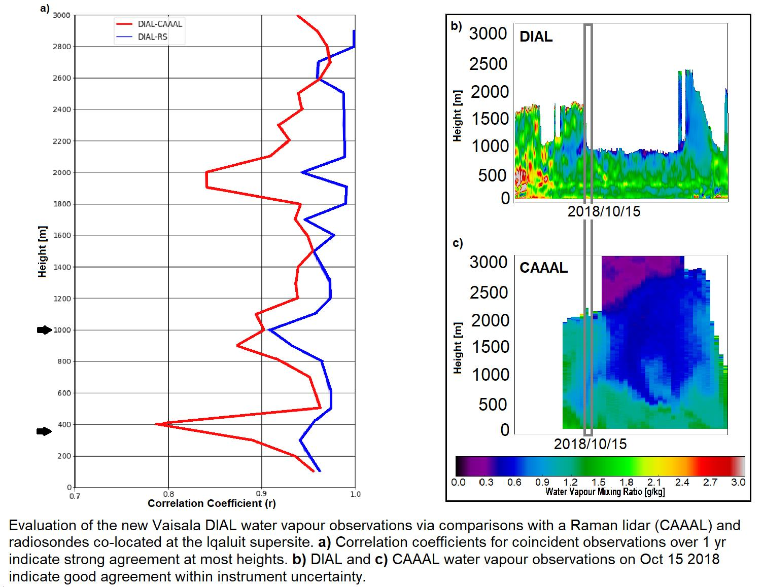
Coincident DIAL-RS and DIAL-CAAAL observations were strongly correlated, as shown in
Figure 9a. This indicates excellent agreement at most heights and is similar to the correlations found in Reference [
26]. For most heights, the correlation between the DIAL and RS is slightly better than the DIAL and CAAAL. The correlation plot at 1000 m AGL (
Figure 9c) demonstrates the typical strong agreement observed for most of the DIAL profile. In contrast, a sudden drop in correlation was observed near the surface (e.g., at 360 m AGL,
Figure 9b), particularly for the DIAL-CAAAL, coinciding with the region of maximum mean bias and STDE in
Figure 6 and
Figure 7.
3.3. Investigation of the DIAL’s Bias
In clear air conditions and during high solar noise levels (e.g., near local noon), the DIAL’s near-range unit suffers from low signal-to-noise ratio (SNR) at its upper heights (>200 m AGL), resulting in an overestimation of the WVMR at heights above 250 m AGL. As such, a small dependency on sunlight was observed in the DIAL’s performance. A statistically significant diurnal bias with a maximum amplitude of 0.4 g/kg during the summer was found between 250 and 400 m. In addition, due to the solar background radiation, the DIAL’s maximum range was lower during daytime operation, and DIAL comparisons during winter months, which experience significantly less sunlight, were better (based on its bias, correlation, and STDE) than during the summer. Note that the latter, however, could also be attributed to the increased WVMR concentration (factor of >10) and variability that occurs in the summer months when Frobisher Bay is ice-free and the weather in Iqaluit more closely resembles that of a southern coastal town.
There are two kinds of features in the DIAL WVMR profiles that can be categorized as bias: a local feature (250 to 400 m AGL) and a global feature (entire profile). The local feature only affects the near-field unit: it corresponds to the increased DIAL-RS and DIAL-CAAAL mean bias and STDE in
Figure 6a and
Figure 7 and the drop in correlation (particularly for the DIAL-CAAAL) in
Figure 9a. This local feature is currently under investigation by the instrument manufacturer, Vaisala, and it is likely caused by complications in the retrieval algorithm in the 250 to 400 m AGL region, where the SNR of the near-range unit is at its lowest in the very low atmospheric backscatter conditions (and hence even lower SNR) experienced in the dry Arctic.
The nature of the DIAL’s global bias affects the entire WVMR profile and produces a consistent positive bias throughout the entire DIAL profile, regardless of time of day or season (
Figure 3,
Figure 6 and
Figure 7). Uncertainties in the spectral analyzer’s resolution decreased the accuracy of the laboratory measurements of the laser spectral width for the near- and far-field units. An overestimation of the laser spectral width resulted in an overestimation of WVMR values, causing this global bias. Vaisala is nearing completion of an updated WVMR retrieval algorithm that, among other improvements, remedies this global bias by reducing the laser spectral width in the retrieval from 0.21/0.20 nm (near/far-range) to 0.20/0.19 nm. The effect of this change produces a small overall shift of the profile towards slightly lower WVMR values, as shown in
Figure 10. 20 June 2019 was chosen as an example because of its stable meteorological conditions, PBL height, and mostly clear skies, as evident from the attenuated backscatter observations (
Figure 10a). For this case, the relative difference between the reprocessed (red) and original (blue) DIAL WVMR profile ranges between −3.0% (0.22 g/kg) near the surface and 0 at the DIAL’s maximum effective range. This change would shift the DIAL’s mean bias profile in
Figure 6a and
Figure 7, centering it closer to zero.
3.4. Year of Polar Prediction: Verification of Numerical Weather Prediction Models Using the DIAL
Using a similar experimental design as the NWP model verification case study via Doppler lidar wind profiles [
29], almost one year of comparisons (7 September 2018 to 22 August 2019) between the RDPS, HRDPS, and CAPS model output and the DIAL WVMR profile observations were performed. The goal of these comparisons was to verify NWP model WVMR output as part of the YOPP project. To perform comparisons with the DIAL, output from each model’s grid point closest to the lidar was compared against all available DIAL observations, which were averaged in 30 m bins to better match the models’ vertical resolution. The models’ WVMR was linearly interpolated to 90, 150, and 300 m AGL, and then every 300 m above that up until 3 km AGL.
The mean bias (model output–DIAL) and STDE, based on the models’ 3 h lead-time forecast, indicate good agreement between the DIAL and all three models (
Figure 11). The maximum number of comparisons (332) was near the surface, and results above 2.5 km are not considered reliable due to the small number of comparisons (<15). The average bias (model–DIAL) was −0.19 ± 0.02, −0.16 ± 0.02, and −0.15 ± 0.02 g/kg for the RDPS, HRDPS, and CAPS models, respectively. Consistent with the DIAL-RS and DIAL-CAAAL comparisons, a small negative bias for the NWP models was observed throughout most of the vertical profile, which was expected considering the DIAL’s wet bias compared to the assimilated RS observations. The higher-resolution HRDPS and CAPS models exhibited only slightly smaller mean biases compared to RDPS. The three models’ biases diverged, with CAPS demonstrating the best performance, near the surface (~400 m AGL) and above 1.25 km AGL. Almost no difference between the different models’ STDE was observed. Similar results were obtained for comparisons against longer lead-time forecasts, albeit with slightly larger mean biases and STDE (not shown).
Seasonal differences in the model–DIAL agreement were observed. Differences were most apparent when comparing results from the winter (DJF = December, January, February) and summer (JJA = June, July, August), as shown in
Figure 12. This highlights differences in the model’s performance during these two very different seasons with extremely dry Arctic conditions and moist coastal conditions, respectively. Results shown are for comparisons at 600 m AGL but are representative of the agreement at most heights. Good agreement was found, particularly for the higher-resolution HRDPS and CAPS models, for most forecast lead times. As the forecast hour increased, the performance of the low-resolution (RDPS) and high-resolution (HRDPS, CAPS) models diverged, with increasing biases for RDPS during the winter and increasing STDE for all models in the summer. The agreement during the winter was better than during the summer for all models, and significantly more variability in the bias and STDE also occurred during the summer.
4. Discussion
During its year-long evaluation, the DIAL measured extremely low WVMRs during the Arctic winter (<1 g/kg) and relatively high concentrations (>8 g/kg) during the summer, including frequent large (factor of 2 to 4) and rapid changes over <5 h. In the October 2018 case study, steep gradients and sudden changes in the WVMR structure, similar to the change in the DIAL’s WVMR profile during a passing cold front in Toronto [
23], was observed by both lidars. Only the DIAL was capable of conducting continuous WVMR observations without large temporal gaps, albeit at altitudes limited to within the PBL. This demonstrates the usefulness of the DIAL’s 24 h observations, its ability to measure fast-moving meteorological features and steep gradients in the WVMR profile, and its ability to fill the temporal gap in water vapor profile observations at WMO RS observation sites. This is particularly important for Iqaluit, where persistent stratified wind and water vapor layers can cause larger model forecast errors [
45].
As a boundary layer profiling instrument, the DIAL exhibited a limited vertical range compared to the CAAAL. Sometimes the DIAL’s WVMR values increased near the DIAL’s maximum range (
Figure 3), and these were associated with a large (>50%) difference between the DIAL and CAAAL in
Figure 3c, d (e.g., just below 1 km at ~10:00 UTC on 16 October 2018). Often, it was found that the DIAL’s quality control algorithm overestimated its maximum effective range by up to 80 m. Further refinement of the quality control algorithm is under development as some potential causes, such as a bright cloud bottom capping the DIAL profile, have been identified.
Large differences between the DIAL and CAAAL’s WVMR observations were also observed when stratified water vapor layers were present on October 13 (
Figure 3 and
Figure 5). This demonstrates a limitation in the DIAL’s ability to resolve these fine structures due to its coarser vertical resolution compared to the CAAAL (the RS did not observe the same layers as the CAAAL, likely because it quickly drifted over Frobisher Bay and sampled a different air mass). However, this period of large disagreement was short-lived and not typical, as evident from the rest of
Figure 3d.
On average, the DIAL-RS and DIAL-CAAL agreed within <±0.3 g/kg for almost all heights (
Figure 6a and
Figure 7). While the DIAL-RS comparisons had a smaller average bias than the DIAL-CAAAL, the DIAL-RS bias profile exhibited more structure and variability, including oscillations and a greater STDE, particularly at higher altitudes. This can likely be attributed to the fewer number of DIAL-RS comparisons and the drifting RS that at times sampled a different air mass. Aside from these features, the similar agreement between the DIAL-RS and DIAL-CAAAL was expected given that the CAAAL used the Iqaluit RS to calibrate its measurements. Note that the DIAL measurements were completely independent of the RS.
The worst agreement occurred between 250 and 400 m AGL, where the majority of large artifacts in the DIAL observations were found, which were more prominent during the winter when WVMR values were lower. This local bias feature is caused by the overlap (near- and far-field) function and is under investigation by Vaisala. The DIAL’s global positive bias, which Vaisala is developing an updated WVMR retrieval algorithm to reduce, could also be partially attributed to a possible dry bias in the RS data, which is yet to be characterized (if it exists) for the new RS model used in this study.
Overall, the performance of the DIAL in Iqaluit is similar to previous evaluations in southern latitudes using the same DIAL and a Raman lidar [
29] and for the prototype DIAL, RSs, and a Raman lidar [
26]. In particular, the shape of the DIAL’s positive mean bias profile and the larger bias and STDE below 400 m (including oscillations in the WVMR profile) were also found in these studies. Artifacts and oscillations in the DIAL profile were more prominent in this study due to the lower WVMR concentrations. The Vaisala DIAL’s results are also similar to an evaluation study of another DIAL system performed in Montana, the MicroPulse DIAL [
20]. This suggests that, with the exception of the 250 to 400 m AGL region, the performance of the Vaisala pre-production DIAL system during extremely dry Arctic conditions is consistent with its performance (and the performance of other similar systems) in southern latitudes.
A verification case study of the ECCC operational NWP forecast at 3 h lead-time using the DIAL WVMR observations showed good agreement (<±0.4 g/kg for most heights) that was slightly better for the higher-resolution models (HRDPS and CAPS). The three models, however, were nearly indistinguishable in terms of their STDE at these short lead-times. Despite its lower resolution, the RDPS still exhibited good agreement with the DIAL observations. All three models exhibited relatively high differences at 0 h lead-time; while one would expect better agreement at 0 h followed by degradation with time, the models assimilate RS data at 0 h, which has a DIAL-RS bias. Overall, the model–DIAL differences were only slightly larger than for the DIAL-RS and DIAL-CAAAL, exhibiting similar features in their bias and STDE profiles.
Similar to the DIAL-RS and DIAL-CAAAL comparisons, the models performed better during the winter than the summer. HRDPS and CAPS exhibited a diurnal cycle in the summer-time bias, not present in RDPS, and this is likely due to differences between the models’ physical processes and resolution. All models exhibited slight increases in their negative bias in winter, and an increase of STDE with forecast lead-time in summer. In contrast, a previous verification case study of wind profiles above Iqaluit showed better model performance in the summer and almost no change in bias with forecast lead-time [
29]. For winds, the daily oscillation in biases and STDE was typically a stronger signal than the forecast error increase with lead-time. The better model performance observed during the winter for WVMR is likely due to the smaller and relatively stable amounts of WVMR that make it easier to forecast.
5. Conclusions
A new, pre-production Vaisala DIAL system underwent a year-long evaluation at the Environment and Climate Change Canada (ECCC)’s Iqaluit supersite. This is the only multi-season evaluation of Vaisala’s pre-production DIAL system and the first evaluation of an autonomous, operational water vapor profiling DIAL system in the harsh Arctic climate. The goal of this study was to investigate the DIAL’s ability to complement existing radiosonde (RS) observations and be deployed as part of an operational network. This evaluation of the DIAL provides a characterization of its error statistics in the Arctic during both extremely dry and moderately humid conditions, as required for NWP model evaluation and assimilation, which is the focus of future work.
The Vaisala DIAL design presents several advantages over existing DIAL designs. Its size makes it relatively portable compared to most systems, which are usually around 2 to 3 times larger. It demonstrated an ability to operate continuously without operator intervention in extreme polar conditions (where historically, observations have been difficult to acquire) down to −40 °C. As of yet, it is the only autonomous water vapor DIAL capable of continuous profiling that is commercially available, which makes it a viable candidate to be used as part of a lidar network. The vertical resolution of the Vaisala DIAL is also comparable to, if not slightly greater than (in the first 1 km), other new DIALs (e.g., [
19]).
DIAL water vapor mixing ratio (WVMR) profile observations were compared against coincident RS observations and a Raman lidar, the Canadian Autonomous Arctic Aerosol lidar (CAAAL), at ECCC’s Iqaluit supersite. With the exception of observations conducted between 250 and 400 m AGL, reliable WVMR measurements were conducted autonomously during extremely dry (<1 g/kg) and relatively moist (>8 g/kg) conditions, including frequent periods of sudden changes. The DIAL typically provided reliable observations from 90 to 250 m AGL and from 400 m up to its maximum range (data availability was >50% for heights below 900 m), with a few exceptions (e.g., during stratified water vapor layers).
On average, good agreement between the DIAL-RS (7 September 2018 to 22 August 2019) and DIAL-CAAAL (7 September 2018 to 27 February 2019) was found, particularly given the difficulty in measuring such low WVMR concentrations. The mean bias was +0.13 ± 0.01 g/kg and +0.18 ± 0.02 g/kg for the DIAL-RS and DIAL-CAAAL, respectively. Observations were also strongly correlated (r > 0.8 for almost all heights below 3 km AGL). These results are consistent with the shorter inter-comparison campaigns performed at southern latitudes in previous studies.
The DIAL exhibited a small but consistent global positive bias, measuring slightly greater WVMR values regardless of altitude, season, or meteorological conditions. This global positive bias is caused by overestimating the laser spectral width in the WVMR retrieval algorithm. Vaisala is developing an updated algorithm that utilizes a smaller laser spectral width: the retrieved WVMR profile was reduced by up to 3% throughout the profile using this updated algorithm. A local bias feature containing large artifacts between 250 and 400 m was also found, exhibiting a statistically significant diurnal cycle. This local bias feature is under current investigation. The updated WVMR retrieval algorithm is expected to address and mitigate both the global and local bias features, and it will be released in the near future and utilized on all future commercial DIAL units.
Once the DIAL’s bias was characterized, its data was used to provide enhanced meteorological observations for model verification and process studies during the World Meteorological Organization’s Year of Polar Prediction (YOPP). DIAL WVMR profiles were compared to ECCC’s Numerical Weather Prediction (NWP) model output and showed good agreement, with the magnitude of their mean biases similar to the DIAL-RS and DIAL-CAAAL comparisons (e.g., −0.15 ± 0.02 g/kg for HRDPS-DIAL), but opposite sign. Since the models assimilated RS data, the NWP models’ negative bias compared to the DIAL was expected and can be partially attributed to the DIAL’s wet bias. The higher-resolution models exhibited better performance with smaller biases and STDE, which is expected for local variables such as planetary boundary layer (PBL) WVMR. All models performed better during the winter than the summer due to the extremely low and stable WVMR values in the Arctic winter compared to the summer.
This study provides strong evidence for the DIAL to complement existing RS observations. The DIAL demonstrated the ability to fill crucial gaps in PBL observations with an accuracy, on average, close to that of a RS (outside of 250 to 400 m AGL) autonomously, reliably (zero instrument failures over the one-year period), and at significantly higher temporal resolution during all weather conditions. Additional applications of the DIAL’s observations are being explored, including an investigation of the DIAL’s ability to accurately quantify height-resolved diurnal water vapor cycles, the results of which will be presented in a subsequent paper. Another significant application of the DIAL’s observations is their ability to fill the 12 h gaps in the ECCC NWP assimilation cycle, which currently lacks observations of sudden changes in the WVMR structure within the PBL brought on by fast-moving meteorological events such as lake breezes, cold fronts, or convective systems. As such, the feasibility of assimilating DIAL WVMR observations into ECCC’s NWP model is under current investigation.
Author Contributions
Conceptualization, Z.M., S.H.-J., and K.S.; methodology, all; formal analysis, Z.M., S.H.-J., J.G., R.W.C., K.S., and B.C.; writing—original draft preparation, Z.M.; writing—review and editing, all. All authors have read and agreed to the published version of the manuscript.
Funding
This research received no external funding.
Data Availability Statement
All data products are produced by ECCC and are available via obrs.ca,
https://yopp.met.no/node/54 (accessed on 13 November 2020), or upon request.
Acknowledgments
Special thanks to Sorin Pinzariu, Michael Harwood, Robert Reed, Reno Sit, Jason Iwachow, Michael Travis, and Daniel Coulombe for their help with instrumentation at the Iqaluit site. Thank you to Peter Rodriguez for processing RS data and the Meteorological Service of Canada RS operators at Iqaluit for launching the RS balloons.
Conflicts of Interest
The instrument manufacturer had no role in the design of the study; in the collection, analyses, or interpretation of data used to perform the instrument or model comparisons; in the writing of the manuscript, or in the decision to publish the results.
References
- Dessler, A.E.; Zhang, Z.; Yang, P. Water vapor climate feedback inferred from climate fluctuations, 2003–2008. Geophys. Res. Lett. 2008, 35, L20704. [Google Scholar] [CrossRef]
- Hwang, Y.-T.; Frierson, D.M.W. Increasing atmospheric poleward energy transport with global warming. Geophys. Res. Lett. 2010, 37, L24807. [Google Scholar] [CrossRef]
- Weaver, D.; Strong, K.; Schneider, M.; Rowe, P.M.; Sioris, C.; Walker, K.A.; Mariani, Z.; Uttal, T.; McElroy, C.T.; Vömel, H.; et al. Intercomparison of atmospheric water vapour measurements at a Canadian High Arctic site. Atmos. Meas. Tech. 2017, 10, 2851–2880. [Google Scholar] [CrossRef]
- National Research Council. Weather Services for the Nation: Becoming Second to None; National Academies Press: Washington, DC, USA, 2012; p. 86. [CrossRef]
- Wulfmeyer, V.; Hardesty, R.M.; Turner, D.D.; Behrendt, A.; Cadeddu, M.P.; Di Girolamo, P.; Schlussel, P.; Van Baelen, J.; Zus, F. A review of the remote sensing of lower tropospheric thermodynamic profiles and its indispensable role for the understanding and the simulation of water and energy cycles. Rev. Geophys. 2015, 53, 819–895. [Google Scholar] [CrossRef]
- Melfi, S.H. Remote measurements of the atmosphere using Raman scattering. Appl. Opt. 1972, 11, 1605–1610. [Google Scholar] [CrossRef]
- Whiteman, D.N. Examination of the traditional Raman lidar technique II Evaluating the ratios for water vapor and aerosols. Appl. Opt. 2003, 42, 2593. [Google Scholar] [CrossRef] [PubMed]
- Bosenberg, J. Ground-based differential absorption lidar for water-vapor and temperature profiling: Methodology. Appl. Opt. 1998, 37, 3845–3860. [Google Scholar] [CrossRef] [PubMed]
- Lazzarotto, B.; Frioud, M.; Larchevêque, G.; Mitev, V.; Quaglia, P.; Simeonov, V.; Thompson, A.; van den Bergh, H.; Calpini, B. Ozone and water-vapor measurements by Raman lidar in the planetary boundary layer: Error sources and field measurements. Appl. Opt. 2001, 40, 2985–2997. [Google Scholar] [CrossRef] [PubMed]
- Whiteman, D.N.; Melfi, S.H.; Ferrare, R.A. Raman lidar system for the measurement of water vapor and aerosols in the Earth’s atmosphere. Appl. Opt. 1992, 31, 3068–3082. [Google Scholar] [CrossRef] [PubMed]
- Whiteman, D.N.; Rush, K.; Veselovskii, I.; Cadirola, M.; Comer, J.; Potter, J.R.; Tola, R. Demonstration Measurements of Water Vapor, Cirrus Clouds, and Carbon Dioxide Using a High-Performance Raman Lidar. J. Atmos. Ocean. Technol. 2007, 24, 1377–1388. [Google Scholar] [CrossRef][Green Version]
- Hicks-Jalali, S.; Sica, R.J.; Martucci, G.; Barras, E.M.; Voirin, J.; Haefele, A. A Raman lidar tropospheric water vapour climatology and height-resolved trend analysis over Payerne, Switzerland. Atmos. Chem. Phys. 2020, 20, 9619–9640. [Google Scholar] [CrossRef]
- Browell, E.V.; Ismail, S.; Grant, W.B. Differential absorption lidar (DIAL) measurements from air and space. Appl. Phys. B 1998, 67, 399–410. [Google Scholar] [CrossRef]
- Karapuzikov, A.; Malov, A.N.; Sherstov, I.V. Tunable TEA CO2 laser for long-range DIAL lidar. IR Phys. Tech. 2000, 41, 77–85. [Google Scholar] [CrossRef]
- Godin-Bekmann, S.; Porteneuve, J.; Garnier, A. Systematic DIAL lidar monitoring of the stratospheric ozone vertical distribution at Observatoire de Haute-Provence (43.92°N, 5.71°E). J. Environ. Monit. 2002, 5, 57–67. [Google Scholar] [CrossRef]
- Machol, J.; Ayers, T.; Schwenz, K.T.; Koenig, K.W.; Hardesty, R.M.; Senff, C.J.; Krainak, M.A.; Abshire, J.B.; Bravo, H.E.; Sandberg, S.P. Preliminary measurements with an automated compact differential absorption lidar for profiling water vapour. App. Opt. 2014, 45, 3110. [Google Scholar]
- Nehrir, A.; Repasky, K.S.; Carlsten, J.L.; Obland, M.D.; Shaw, J.A. Water vapour profiling using a widely tuneable amplified diode-laser based differential absorption lidar (DIAL). J. Atmos. Ocean. Tech. 2009, 26, 737–745. [Google Scholar] [CrossRef]
- Baron, P.; Ishii, S.; Mizutani, K.; Itabe, T.; Yasui, M. Profiling tropospheric water vapour with a coherent infrared differential absorption lidar: A sensitivity analysis. In Proceedings of the Lidar Remote Sensing for Environmental Monitoring XIII, Kyoto, Japan, 29 October–1 November 2012; Volume 8526, p. 85260D. [Google Scholar] [CrossRef]
- Spuler, S.M.; Repasky, K.S.; Morley, B.; Moen, D.; Hayman, M.; Nehrir, A.R. Field-deployable diode-laser-based differential absorption lidar (DIAL) for profiling water vapor. Atmos. Meas. Tech. 2015, 8, 1073–1087. [Google Scholar] [CrossRef]
- Weckwerth, T.M.; Weber, K.J.; Turner, D.D.; Spuler, S.M. Validation of a water vapor micropulse differential absorption lidar (DIAL). J. Atmos. Oceanic Technol. 2016, 33, 2353–2372. [Google Scholar] [CrossRef]
- Imaki, M.; Tanaka, H.; Hirosawa, K.; Yanagisawa, T.; Kameyama, S. Demonstration of the 1.53-µm coherent DIAL for simultaneous profiling of water vapor density and wind speed. Opt. Express 2020, 28, 27078–27096. [Google Scholar] [CrossRef] [PubMed]
- Kampfer, N. Monitoring Atmospheric Water Vapour: Ground-Based Remote Sensing and In-Situ Methods; Springer Science: Berlin/Heidelberg, Germany, 2013. [Google Scholar] [CrossRef]
- Mariani, Z.; Stanton, N.; Whiteway, J.; Lehtinen, R. Toronto Water vapour lidar inter-comparison campaign. Remote Sens. 2020, 12, 3165. [Google Scholar] [CrossRef]
- Roininen, R.; Münkel, C. 12.3 Results from continuous atmospheric boundary layer humidity profiling with a compact DIAL instrument. In Proceedings of the Eighth Symposium on Lidar Atmospheric Applications, Seattle, WA, USA, 26 January 2017; American Meteorological Society: Boston, MA, USA, 2017. Available online: https://ams.confex.com/ams/97Annual/webprogram/Paper301717.html (accessed on 13 November 2020).
- Münkel, C.; Roininen, R. Results from continuous atmospheric boundary layer humidity profiling with a compact DIAL instrument. In Proceedings of the European Conference for Applied Meteorology and Climatology, Dublin, Ireland, 27–30 September 2016; European Meteorological Society: Boston, MA, USA, 2016; p. 525. [Google Scholar]
- Newsom, R.K.; Turner, D.D.; Lehtinen, R.; Münkel, C.; Kallio, J.; Roininen, R. Evaluation of a Compact Broadband Differential Absorption Lidar for Routine Water Vapor Profiling in the Atmospheric Boundary layer. J. Atmos. Ocean. Technol. 2020, 37, 47–65. [Google Scholar] [CrossRef]
- Joe, P.; Melo, S.; Burrows, W.; Casati, B.; Crawford, R.; Deghan, A.; Gascon, G.; Mariani, Z.; Milbrandt, J.; Strawbridge, K. The Canadian Arctic Weather Science Project: Introduction to the Iqaluit Site. Bull. Am. Meteorol. Soc. 2020, 101, E109–E128. [Google Scholar] [CrossRef]
- Køltzow, M.; Casati, B.; Bazile, E.; Haiden, T.; Valkonen, T. An NWP model intercomparison of surface weather parameters in the European Arctic during the year of polar prediction special observing period northern hemisphere 1. Weather Forecast. 2019, 34, 959–983. [Google Scholar] [CrossRef]
- Mariani, Z.; Crawford, R.; Casati, B.; Lemay, F. A Multi-year evaluation of Doppler lidar wind-profile observations in the Arctic. Remote Sens. 2020, 12, 323. [Google Scholar] [CrossRef]
- Dabberdt, W.; Kallio, J.; Komppula, M.; Laukkanen, S.; O’Connor, E.J. 8.4. Advances in continuous atmospheric boundary layer humidity profiling with a compact DIAL Instrument. In Proceedings of the 18th Symposium on Meteorological Observation and Instrumentation, New Orleans, LA, USA, 13 January 2016; American Meteorological Society: Boston, MA, USA, 2016. Available online: https://ams.confex.com/ams/96Annual/webprogram/Paper285586.html (accessed on 13 November 2020).
- Strawbridge, K.B. Developing a portable, autonomous aerosol backscatter lidar for network or remote operations. Atmos. Meas. Tech. 2013, 6, 801–816. [Google Scholar] [CrossRef]
- Strawbridge, K.B.; Travis, M.S.; Firanski, B.J.; Brook, J.R.; Staebler, R.; Leblanc, T. A fully autonomous ozone, aerosol and nighttime water vapor lidar: A synergistic approach to profiling the atmosphere in the Canadian oil sands region. Atmos. Meas. Tech. 2018, 11, 6735–6759. [Google Scholar] [CrossRef]
- Leblanc, T.; Sica, R.J.; van Gijsel, J.A.E.; Godin-Beekmann, S.; Haefele, A.; Trickl, T.; Payen, G.; Gabarrot, F. Proposed standardized definitions for vertical resolution and uncertainty in the NDACC lidar ozone and temperature algorithms—Part 1: Vertical resolution. Atmos. Meas. Tech. 2016, 9, 4029–4049. [Google Scholar] [CrossRef]
- GRAW. 2020. Available online: https://www.graw.de/products/radiosondes/dfm-09/ (accessed on 22 October 2020).
- Wang, J.; Zhang, L.; Dai, A.; Immler, F.; Sommer, M.; Vomel, H. Radiation dry bias correction of Vaisala RS92 humidity data and its impacts on historical radiosonde data. J. Atmos. Ocean. Technol. 2013, 30, 197–214. [Google Scholar] [CrossRef]
- Côté, J.; Gravel, S.; Méthot, A.; Patoine, A.; Roch, M.; Staniforth, A. The operational CMC–MRB Global Environmental Multiscale (GEM) model: Part I. Design considerations and formulation. Mon. Weather Rev. 1998, 126, 1373–1395. [Google Scholar] [CrossRef]
- Girard, C.; Plante, A.; Desgagne, M.; McTaggart-Cowan, R.; Cote, J.; Charron, M.; Gravel, S.; Lee, V.; Patoine, A.; Qaddouri, A.; et al. Staggered Vertical Discretization of the Canadian Environmental Multiscale (GEM) model using a coordinate of the log-hydrostatic-pressure type. Mon. Weather Rev. 2014, 142, 1183–1196. [Google Scholar] [CrossRef]
- Bélair, S.; Crevier, L.-P.; Mailhot, J.; Bilodeau, B.; Delage, Y. Operational implementation of the ISBA land surface scheme in the Canadian regional weather forecast model. Part I: Warm season results. J. Hydrometeorol. 2003, 4, 352–370. [Google Scholar] [CrossRef]
- Buehner, M.; McTaggart-Cowan, R.; Beaulne, A.; Charette, C.; Garand, L.; Heilliette, S.; Lapalme, E.; Lapalme, E.; Macpherson, S.R.; Zadra, A.; et al. Implementation of deterministic weather forecasting systems based on ensemble–variational data assimilation at Environment Canada. Part I: The global system. Mon. Weather Rev. 2015, 143, 2532–2559. [Google Scholar] [CrossRef]
- Smith, G.C.; Roy, F.; Reszka, M.; Colan, D.S.; He, Z.; Deacu, D.; Belanger, J.-M.; Skachko, S.; Liu, Y.; Dupont, F.; et al. Sea ice forecast verification in the Canadian Global Ice Ocean Prediction System. Q. J. R. Meteorol. Soc. 2016, 142, 659–671. [Google Scholar] [CrossRef]
- Dupont, F.; Higginson, S.; Bourdallé-Badie, R.; Lu, Y.; Roy, F.; Smith, G.C.; Lemieux, J.-F.; Garric, G.; Davidson, F. A high-resolution ocean and sea-ice modelling system for the Arctic and North Atlantic oceans. Geosci. Model Dev. 2015, 8, 1577–1594. [Google Scholar] [CrossRef]
- Lemieux, J.-F.; Beaudoin, C.; Dupont, F.; Roy, F.; Smith, G.C.; Shlyaeva, A.; Buehner, M.; Caya, A.; Chen, J.; Carrieres, T.; et al. The Regional Ice Prediction System (RIPS): Verification of forecast sea ice concentration. Q. J. R. Meteorol. Soc. 2016, 142, 632–643. [Google Scholar] [CrossRef]
- Morrison, H.; Milbrandt, J. Parameterization of cloud microphysics based on the prediction of bulk ice particle properties. Part I: Scheme description and idealized tests. J. Atmos. Sci. 2015, 72, 287–311. [Google Scholar] [CrossRef]
- Milbrandt, J.; Morrison, H. Parameterization of cloud microphysics based on the prediction of bulk ice particle properties. Part III: Introduction of multiple free categories. J. Atmos. Sci. 2016, 73, 975–995. [Google Scholar] [CrossRef]
- Mariani, Z.; Dehghan, A.; Gascon, G.; Joe, P.; Hudak, D.; Strawbridge, K.; Corriveau, J. Multi-instrument observations of prolonged stratified wind layers at Iqaluit, Nunavut. Geophys. Res. Lett. 2018, 45, 1654–1660. [Google Scholar] [CrossRef]
Figure 1.
Summer 2019 satellite image of the region surrounding Iqaluit (left) and a zoomed-in image of the Iqaluit supersite (insert), indicating locations of the Canadian Autonomous Arctic Aerosol Lidar (CAAAL) (1), radiosonde (RS) launch site (2), differential absorption lidar (DIAL) (3), and surface meteorological instruments used in this study. The Iqaluit airport (with code CYFB) runway is ~200 m to the NE of the supersite. Copyright: 2020 CNES/Airbus, Maxar Technologies, Google Maps.
Figure 2.
The pre-production Vaisala DIAL system (left) and the CAAAL (right) operating at the Iqaluit supersite. The CAAAL photo taken during long exposure enhances white lights from the airport in the background: Daniel Coulombe (ECCC).
Figure 2.
The pre-production Vaisala DIAL system (left) and the CAAAL (right) operating at the Iqaluit supersite. The CAAAL photo taken during long exposure enhances white lights from the airport in the background: Daniel Coulombe (ECCC).
Figure 3.
DIAL (a) and CAAAL (b) WVMR profile observations from 13 to 17 October 2018. Note the fine WVMR color bar scale. The percent difference between the DIAL-CAAAL (c) and the absolute difference (d) are shown below. DIAL data above its maximum effective range and CAAAL data with uncertainty > 25% have been removed and capped at 3 km for comparison purposes. Gaps in the CAAAL data occur during sunlight, when WVMR measurements are not possible. The time of 00 and 12 UTC RS observations (grey vertical lines) are also shown. Red arrows mark the time of the individual profile comparison in Figure 5.
Figure 4.
Similar to
Figure 3, except for DIAL 911 nm (
a) and CAAAL 532 nm (
b) attenuated backscatter profile observations from 13 to 17 October 2018. Note the backscatter scales in (
a,
b) are different. Red arrows mark the time of the individual profile comparisons in
Figure 5.
Figure 4.
Similar to
Figure 3, except for DIAL 911 nm (
a) and CAAAL 532 nm (
b) attenuated backscatter profile observations from 13 to 17 October 2018. Note the backscatter scales in (
a,
b) are different. Red arrows mark the time of the individual profile comparisons in
Figure 5.
Figure 5.
(a) 20 min averaged (11:20–11:40 UTC) WVMR profiles as measured by the DIAL (blue), CAAAL (red), and radiosonde launched at 11:20 UTC (black) on 13 October 2018 when stratified water vapor layers were present. The shaded region represents the uncertainty in the DIAL profile (not shown for the CAAAL or RS for clarity). The absolute (b) and percent (c) difference between the DIAL-CAAAL (red) and DIAL-RS (black) are shown alongside the DIAL uncertainty (blue).
Figure 6.
(a) DIAL-RS (blue) and DIAL-CAAAL (red) bias and standard deviation of the error (STDE, shaded region) for coincident (night-time only) observations from 7 September 2018 to 27 February 2019. (b) Number of comparisons for the DIAL-RS (blue) and the DIAL-CAAAL (red).
Figure 6.
(a) DIAL-RS (blue) and DIAL-CAAAL (red) bias and standard deviation of the error (STDE, shaded region) for coincident (night-time only) observations from 7 September 2018 to 27 February 2019. (b) Number of comparisons for the DIAL-RS (blue) and the DIAL-CAAAL (red).
Figure 7.
Same as
Figure 6a, except for the full year (including daytime) of DIAL-RS comparisons (all comparisons between 7 September 2018 and 22 August 2019).
Figure 7.
Same as
Figure 6a, except for the full year (including daytime) of DIAL-RS comparisons (all comparisons between 7 September 2018 and 22 August 2019).
Figure 8.
The DIAL’s data availability during all available observations from 7 September 2018 to 22 August 2019 (blue). The DIAL (black) and CAAAL’s (red) data availability during the same period of night-time observations from 7 September 2018 to 27 February 2019 is shown for comparison.
Figure 8.
The DIAL’s data availability during all available observations from 7 September 2018 to 22 August 2019 (blue). The DIAL (black) and CAAAL’s (red) data availability during the same period of night-time observations from 7 September 2018 to 27 February 2019 is shown for comparison.
Figure 9.
(a) DIAL-RS (blue) and DIAL-CAAAL (red) correlation coefficients for coincident observations from 7 September 2018 to 27 February 2019. Correlations were binned every 50 m. Black arrows in (a) indicate the heights of the two example correlation plots at 360 m AGL (b) and 1000 m AGL (c). Linear fits and the 1:1 line (black dash) are also shown.
Figure 10.
(a) DIAL attenuated backscatter observations on 20 June 2019 showing stable meteorological conditions and mostly clear skies at Iqaluit. The black box indicates the corresponding region in space and time where the WVMR measurements were calculated for the example reprocessed (red) and original (blue) DIAL WVMR profile at 13:40–14:00 UTC (b).
Figure 11.
Three-hour forecast lead-time model–DIAL mean bias (dashed line) and STDE (solid line) for the RDPS (red), HRDPS (blue), and CAPS (green) model output from 7 September 2018 to 22 August 2019. The mean of the bias profile is also shown (dotted vertical line).
Figure 11.
Three-hour forecast lead-time model–DIAL mean bias (dashed line) and STDE (solid line) for the RDPS (red), HRDPS (blue), and CAPS (green) model output from 7 September 2018 to 22 August 2019. The mean of the bias profile is also shown (dotted vertical line).
Figure 12.
RDPS (red), HRDPS (blue), and CAPS (green) mean model bias (dashed line) and STDE (solid line) compared to the DIAL WVMR profile (model–DIAL) as a function of forecast lead-time at 600 m AGL. Comparisons during the winter are shown in the top two rows (a), and summer comparisons are shown in the bottom two rows (b). Differences between the RDPS and HRDPS mean bias are shown in the lower panels (grey shading indicates 90% confidence intervals). Note the scale for the RDPS and HRDPS difference is 10 times larger for the summer (b) than for the winter (a).
Table 1.
Primary technical specifications of the Vaisala DIAL and CAAAL.
Table 1.
Primary technical specifications of the Vaisala DIAL and CAAAL.
| Lidar | Vaisala DIAL | CAAAL |
|---|
| Dimensions | 1.97 × 0.85 × 0.58 m | ~2 × 1 × 1 m + power supply |
| Weight (including shelter) | 150 kg | ~500 kg |
| Averaging time/reporting interval | 20 min/1 min | 5–20 min/1 min |
| Maximum range: backscatter | 14.4 km | 15 km |
| Typical min/max range: water vapor | 50 m/~3 km | 100 m/~10 km |
| Range reporting interval | 4.8 m | 3.75 m |
| Range resolution | 100–500 m | 29 m up to 1 km |
| Pulse energy | 9 μJ | 115 mJ |
| Pulse repetition rate | 10 kHz | 100 Hz |
| Output wavelengths | 911.0/910.6 nm | 355/532/1064 nm |
| Publisher’s Note: MDPI stays neutral with regard to jurisdictional claims in published maps and institutional affiliations. |
© 2021 by the authors. Licensee MDPI, Basel, Switzerland. This article is an open access article distributed under the terms and conditions of the Creative Commons Attribution (CC BY) license (http://creativecommons.org/licenses/by/4.0/).


 ,
, 


