Article

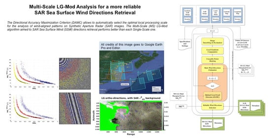
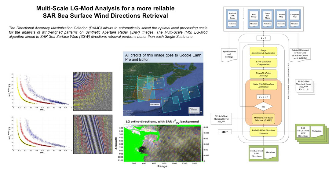
Multi-Scale LG-Mod Analysis for a More Reliable SAR Sea Surface Wind Directions Retrieval

National Research Council of Italy (CNR), Institute of Atmospheric Pollution (IIA), Department of Physics, University of Bari, 70126 Bari, Italy
*
Author to whom correspondence should be addressed.
Remote Sens. 2021, 13(3), 410; https://doi.org/10.3390/rs13030410
Submission received: 2 December 2020 / Revised: 11 January 2021 / Accepted: 22 January 2021 / Published: 25 January 2021
(This article belongs to the Special Issue Remote Sensing of Ocean Surface Winds)

Abstract

:
An improved version of the Local-Gradient-Modified (LG-Mod) algorithm for Sea Surface Wind (SSW) directions retrieval by means of Synthetic Aperture Radar (SAR) images is presented. A “local” multi-scale analysis of wind-aligned SAR patterns is introduced to improve the LG-Mod sensitivity to SAR backscattering modulations, occurring locally with various spatial wavelengths. The Marginal Error parameter is redefined, and the adoption of the Directional Accuracy Maximization Criterion (DAMC) allows for the novel Multi-Scale (MS) LG-Mod to automatically select the local processing scale that may be regarded as optimal for pattern enhancement, once a discrete set of scales has been already fixed. Hence, this optimal scale successfully gives evidence to guarantee the best achievable local direction estimation. The assessment of the MS LG-Mod is carried on both simulated SAR images and a Sentinel-1 (S-1) dataset, consisting of 350 Interferometric Wide Swath Ground Range Multi-Look Detected High-Resolution images, which cover the region of the Gulf of Maine. In the latter case, the removal of artifacts and non-wind features from SAR amplitudes is mandatory before directional estimations. In situ wind observations gathered by the National Oceanic and Atmospheric Administration National Data Buoy Center (NOAA NDBC) are exploited for validation. The findings obtained from S-1 data confirm the ones from simulated patterns. The MS LG-Mod analysis performs better than each single-scale one in terms of both percentages of reliable directions and directional Root Mean Square Error (RMSE) values achieved.

Graphical Abstract

1. Introduction

Sea Surface Wind (SSW) is a very important parameter for studies in many fields of application, such as marine meteorology and oceanography [1], coastal ecosystems monitoring and conservation [2], and wind energy mapping [3].
Among available tools, Synthetic Aperture Radar (SAR) systems are commonly used in most meteorological conditions, and they can provide wind information at high spatial resolution [4,5,6,7,8]. In spite of many methods recently proposed, the approach that exploits the dependency of SAR Normalized Radar Cross-Section (NRCS) on wind parameters (wind speed and direction), and the geometry of acquisitions (radar incidence angle) via empirical Geophysical Model Function (GMF) is still widely used [9,10,11,12,13].
One of the inconveniences of this approach is the requirement of wind direction estimate as an input parameter. In fact, assuming wind direction as a priori information, wind speed can be inferred through the inversion of a GMF. This can lead to errors in SAR wind speed estimation mainly due to those related to wind direction used.
Recently, both the United States National Oceanic and Atmospheric Administration (NOAA) and the European Space Agency (ESA) have implemented an operational service based on the scatterometry-based approach, providing wind field from SAR data exploiting wind direction from Numerical Weather Prediction (NWP) models as input [14,15]. Even though data from NWP models are always available, so to guarantee the operational provision of the service, they can meet problems when used in coastal areas [16].
Another way for the retrieval of wind direction information is the estimation of wind direction directly from SAR images. This methodology has the advantage that wind direction could be provided at high spatial resolutions, in coastal areas where NWP models typically show limitations, in hardly accessible areas where marine buoys are not deployable, and in coincidence with SAR acquisitions as well. Moreover, it has been proven that the use of SAR-derived direction as input in a scatterometry-based approach can improve wind speed estimation in comparison with results obtained by using NWP models direction in two coastal areas [17]. In particular, an improvement of the Root Mean Square Error (RMSE) up to about 2 m/s has been found.
The developed algorithms basically rely upon the estimation of the prevailing local orientation of linear wind induced and aligned SAR signatures, such as those from Boundary Layer Rolls (BLRs) and Wind Streaks (WSs) [18,19]. These features, otherwise termed “wind rows”, could be visible on SAR amplitude in favorable conditions, which are determined by thermal and dynamic air–sea instability and typical wind speed values from 2 m/s, with the highest probability of wind streaks in the SAR images found for wind speeds of about 8–9 m/s [20,21].
Due to the alignment with the mean Sea Surface Wind direction, wind rows are exploited for SAR SSW direction retrieval.
Depending on physical phenomena causing them, these manifestations of the local wind may persist over different times and occur as modulations of the SAR backscattering with various wavelengths ranging from 0.1 to about 9 km [18,22].
As a consequence, an appropriate pixel-size (or scale) for SAR data processing must be identified in order to achieve reliable wind directions retrieval, and a multi-scale analysis of the patterns of interest became crucial.
Several methods were proposed to retrieve wind rows directions from SAR. They include the use of the Fast Fourier Transform (FFT) method [23], the Local Gradient method [22,24], the Wavelet Transform method [25] and those based on the use of texture measurements, such as the Gray-Level Co-Occurrence Matrix (GLCM) derived ones [26].
However, a poor number of studies discussed about the capability to automatically select the optimal processing scale able to adapt the analysis to the ranging scales characterizing the wind rows.
Du et al. [27] exploited the ability of Discrete Wavelet Transform (DWT) to provide a multi-scale analysis of a SAR images for wind direction retrieval. Wavelet texture analysis of the SAR image is performed using the vertical wavelet coefficients with the adoption of different wavelet basis functions (e.g., db4 wavelet decomposition). With the two-dimensional DWT, the SAR image can be decomposed into different scale images, which describe different scale texture features. The scale of the decomposition depends on the scale of the texture features of interest, the pixel spacing, and the size of the original image.
In Reference [28] the decomposition of a SAR image with the Undecimated Wavelets Transform (UWT) and the estimation of the wind direction using the Fourier spectrum were proposed. With this method frequencies of modulations not belonging to the BLR and WS ranges are attenuated.
Noratiqah et al. [29] suggested a multi-resolution analysis along with the application of wavelets transform to handle with multi-scale occurrence of wind rows.
The application of the two-dimensional Continuous Wavelet Transform (CWT) technique was proposed in Reference [30]. This method is applied to a SAR image to obtain the wavelet spectrum, which is the map of energy as a function of angles and scales, the latter chosen in the range between 200 and 2500 m. The scales and angles of the maximum wavelet spectrum are then selected and used to reconstruct the SAR image, which will contain only the spatial features at these scales and angles, i.e., the features of the wind imprinting the sea surface, typically backscatter cells elongated in the wind direction.
In Reference [31] the use of the Non Subsampled Contourlet Transform (NSCT) algorithm for wind direction estimation was proposed. Authors stated that NSCT transform is suitable for the estimation of wind direction from ocean SAR images, which is a typical multi-scale texture analysis problem.
The Local Gradient (LG) method [22] is still one of the most used techniques for wind direction retrieval since it may estimate local wind direction with smaller resolution cells. For each considered scale, one histogram of local directions is built up and the main direction is evaluated. In Reference [32], different option were tried to choose the optimal among estimated directions: (1) to take the direction closest to an available wind direction provided by a NWP model and (2) to take by visual inspection the direction closest to wind-aligned signatures detected on the SAR image.
To the best of our knowledge, the literature that reports the multi-scale analysis of wind rows suffers from several limitations: (1) some of the methods proposed [28,30] implement a multi-scale analysis that has been designed with the aim of enhancing the modulations belonging to the BLRs and WSs, without any effective selection of the optimal scale; (2) one method [32] makes use of a priori external wind information to select the optimal scale among a number of tested ones, thus making the method not fully automatic; (3) the only method [27] for which a selection of the optimal scale is carried out does not present effective comparisons with single-scales performance.
In the present work, a criterion for the optimal scale automatic selection is introduced to overcome all of these issues, supported by a comparison with single-scales performance as well.
In a previous study, Rana et al. [17] proposed the LG-Mod algorithm and investigated the usefulness of the Single-Scale Marginal Error parameter (SS M E α R O I ), in providing an “optimal” SAR processing pixel-size selection for the matching with wind rows modulation wavelengths. This optimal processing scale was identified, among a set of scales, as the single one which can globally yield in a SAR image the largest percentage value of reliable ROIs, i.e., the ROIs characterized by a SS M E α R O I value less than or equal to an established threshold of acceptance M E T H . Nevertheless, it is worth noting that the optimization adopted was not the best. In fact, this first attempt of multi-scale analysis relied on a global approach. The algorithm was limited to choose only one unique single-scale, among an employed set, for the processing of the whole SAR image. It meant, one scale for one SAR image.
However, considering that a full-frame SAR image may cover hundreds of kilometers (for azimuth and range dimensions) and that the actual wind regime conditions may be very different in wide regions, the limitation in Reference [17] was to be overcome. Indeed, since wind rows wavelengths may vary widely depending on several physical factors, such patterns should be considered intrinsically local and locally analyzed as well.
As consequence, this work introduces a newly defined Multi-Scale Marginal Error parameter, i.e., MS M E α R O I , as an indicator for a local choice of the optimal processing scale through a Directional Accuracy Maximization Criterion (DAMC). Differently from the approach in Reference [17], the novel multi-scale analysis is carried out locally and it really allows the processing of a SAR image using multiple scales. This local approach results in the best wind rows enhancement and wind directions estimation performance.
The novel technique is experimented on a valuable Sentinel-1 dataset and exploiting in situ data measured by anemometers on board stations belonging to the NOAA network. Hence, this study deals with the full validation of the technique on real SAR data, also verifying first results obtained on simulated SAR patterns, as presented in Reference [8].
The peculiarity of the “local” MS LG-Mod also allows the method to establish possible spatial correlations between the chosen optimal scale and environmental parameters, such as wind speed and direction, bathymetry and distance from the coast.
The paper is organized as follows: Section 2 describes the procedure used to produce simulated SAR images, the characteristics of the Sentinel-1 dataset, and the available NOAA in situ wind measurements; Section 2 also presents the methodology adopted for extracting wind direction from SAR data and for directional comparison criteria; Section 3 reports results and Section 4 provides their discussion; and Section 5 summarizes the conclusions.

2. Materials and Methods

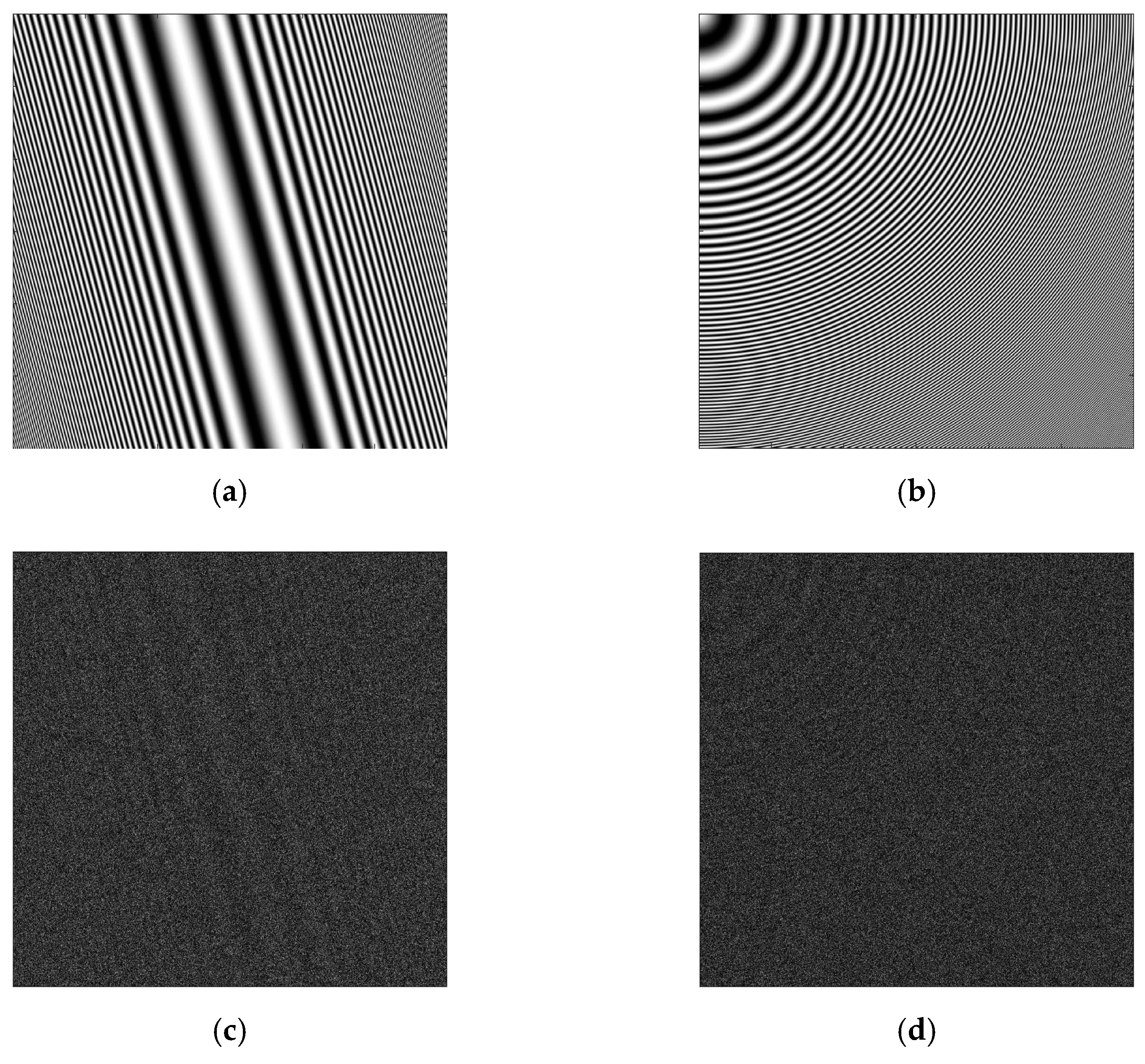
2.1. Simulated SAR Images

Both linear and circular patterns were generated to simulate SAR backscattering modulations observable in real cases of wind-forced patterns visibility [8]. These patterns were characterized by spatial wavelengths in the range (500 m–2 km) for wind rows detection. Typical values of SAR amplitudes over the sea were assumed. A speckle noise, modeled with a Rayleigh distribution, was also taken into account for SAR amplitudes. Simulated images were considered of a 3000 by 3000 (azimuth by range) dimension, simulating a pixel size of 10 m by 10 m.
Patterns obtained are shown in Figure 1a–d, both without and with the multiplicative speckle noise, respectively.

2.2. Sentinel-1 SAR Images

To evaluate wind directions estimation through the LG-Mod algorithm by means of real SAR data, a Sentinel-1 dataset of C-band VV-polarized images was built up. Both ascending and descending images, acquired by both Sentinel-1 (S-1) A and B satellites, were downloaded from the Copernicus Open Access Hub. However, only S-1 Interferometric Wide Swath Ground Range Multi-Look Detected High-Resolution (henceforth, IW) images were chosen, since SS LG-Mod directional performance analysis already indicated that IW images (with 10 m by 10 m resolution) are the optimal choice for high-resolution SSW retrieval [17].
The Sentinel-1 dataset spans from 17th June 2015 to 20th April 2018 and covers the Gulf of Maine region (Northeastern America). Sentinel-1 frames that cover the available in situ measurement stations, i.e., S1B-10391-40-1/2 (descending pass), S1A-21484-62-1/2/5/6, S1B-10515-164-6, S1A-6740-18-1, S1A-15417-120-5, and S1A-7513-91-1 (ascending passes), were selected. Hence, a Sentinel-1 dataset consisting of 350 IW images was obtained. The full-frame coverage of the all selected images is shown in Figure 2.

2.3. In Situ Data

Wind observations gathered by the in situ stations of the National Oceanic and Atmospheric Administration National Data Buoy Center (NOAA NDBC) were exploited to assess the performance of the MS LG-Mod processing. Wind measurements were provided at the reference height of 10 m above the mean sea level, with both different time intervals between acquisitions and directional accuracies depending on the stations equipment, as reported in Table 1. This table reports also the geographic location and further information of the 17 stations matching in time and space with the Sentinel-1 acquisitions. Deployment of the NOAA NDBC stations is shown in Figure 2.

2.4. Multi-Scale LG-Mod Processing

The MS LG-Mod processing scheme is reported in Figure 3. The input to the algorithm consists in a single SAR image, which could be either a simulated one or a co-polarized (VV or HH) Sentinel-1 Normalized Radar Cross-Section (NRCS) image. The latter must be accompanied by auxiliary products (i.e., land–sea mask and, latitude and longitude maps), e.g., obtained using the Sentinel Application Platform (SNAP) freely available from the European Space Agency (ESA). In particular, land–sea mask is exploited to mask out the land from processing. Latitude and longitude maps are used instead to finally provide geographical location for output wind estimations, since the processing is completely carried out in SAR geometry (i.e., on azimuth by range images).
The main processing steps of the MS LG-Mod algorithm are reported in the following:
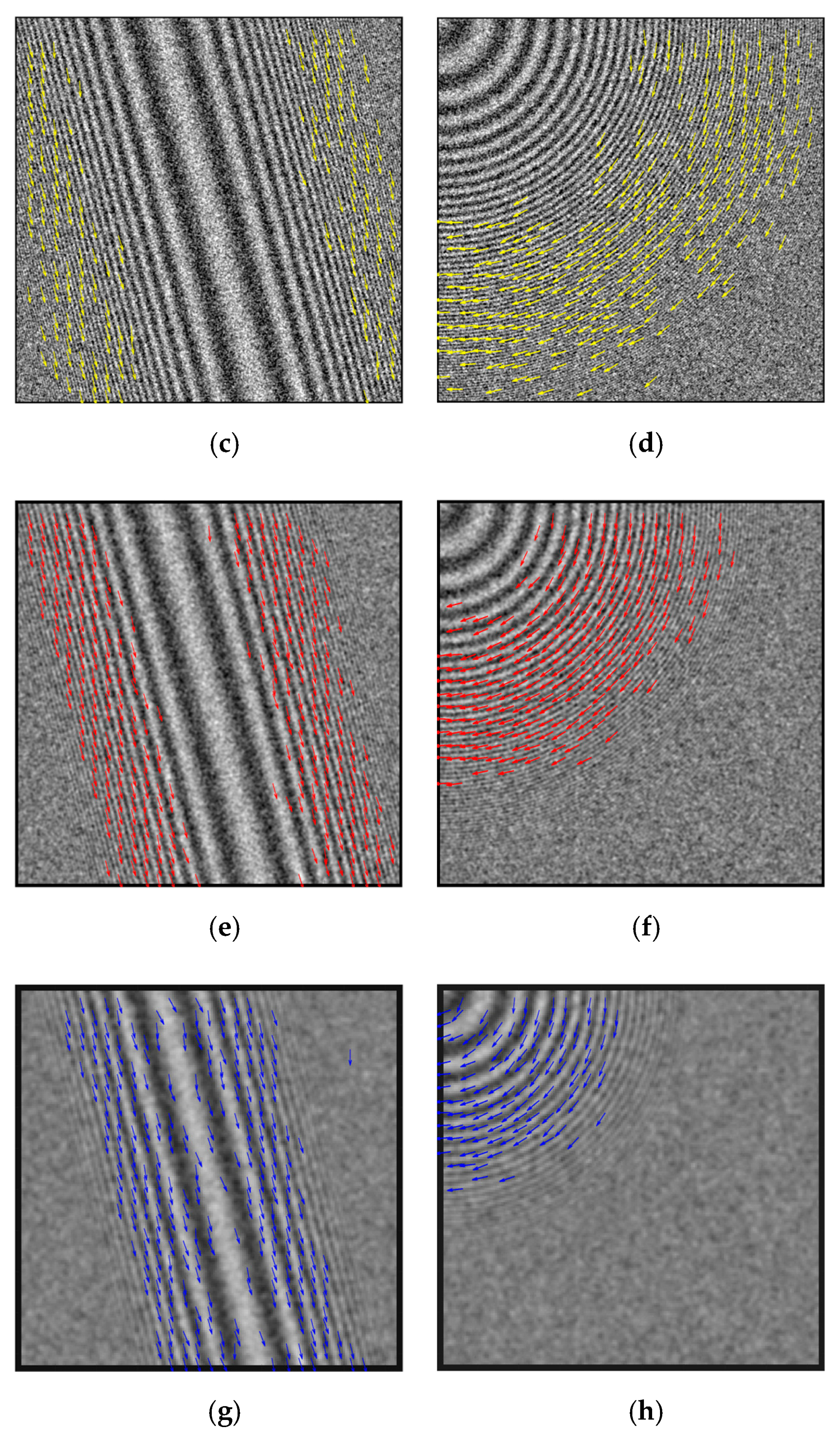
  • Image Smoothing and Decimation [8,17]: This step consists in a series of smoothing and sub-sampling operations with the aim at both enhancing patterns of interest and reducing the speckle noise of the input SAR image. Smoothing operations are edge preserving in order to preserve as much as possible the directional information of the wind-induced SAR signatures. Sub-sampling (with factor 2) reduces by half both the image dimensions as well as it doubles the (final) scale in both dimensions themselves. To capture SAR wind rows characterized by wavelengths in the range between 500 m and 2 km, slightly smaller than the one chosen in Reference [30], scales are profitably selected spanning the range from about 100 to 400 m. Note that the use of higher scales would introduce too much smoothing, thus leading to an unpleasant directional information loss, and a large reduction on the number of samples for directional estimations as well. Lower scales instead would cause noisy estimations, although with a large number of samples. As consequence, for the available Sentinel-1 dataset, S = 3 processing scales, i.e., the High Scale (320 m by 320 m), the Medium Scale (160 m by 160 m), and the Low Scale (80 m by 80 m), were selected for wind rows detection. However, this step may be generally repeated with a different number S of scales, i.e., k { 1 , , S } .
  • Local Gradients Computation [17,22]: This computation is performed for each previously resized image (one image for each k-th scale applied). Local Gradients (LGs) that correspond to “unusable points” are discarded in the next step.
  • Unusable Points Masking (UPM): At this step, land pixels from the available land–sea mask and those affected by unwanted border effects as a result of the filtering performed at the first step are masked. Furthermore, the masking of those points characterized by extremely high or extremely low Local Gradients is carried out. A thresholding is aimed at excluding most of the sigma nought modulations and LGs that are not related to wind rows. To accomplish this task the condition of 2 × 10 4 < A m p l i t u d e ( L G ) < 2 × 10 3 (with experimentally determined thresholds) is required for each pixel within each sub-image (or ROI) to be evaluated in the subsequent steps.
  • Main Wind Directions Estimation: Previous steps are repeated for a number S of selected scales, i.e., k { 1 , , S } . Each LG direction image obtained from each of such repetition is divided into ROIs. Those ROIs that are affected by a large percentage of unusable points detected (e.g., more than 30%) are discarded and related estimations are not provided. Otherwise, for each k-th LG direction image as well as for each not-discarded ROI, a confidence interval is provided with a user-defined confidence level ( 1 α ) , as follows:
    β R O I , k ± M E α R O I , k
Hence, given the set of N R O I , k (usable) LG directions, i.e., { β i R O I , k } i = 1 N R O I , k , the local directional estimate, i.e., β R O I , k , and the semi-width of the related confidence interval, i.e., the Single-Scale Marginal Error, M E α R O I , k , are expressed in radians by the following equations, respectively:
β R O I , k = 1 2 arctan 2 ( sin ( 2 β i R O I , k ) , cos ( 2 β i R O I , k ) )
M E α R O I , k = 1 2 arcsin ( u α ( 1 α 2 R O I , k ) 2 N R O I , k ( R R O I , k ) 2 )
where u α is the upper 1 2 α quintile of the standard normal distribution, and α 2 R O I , k represents the 2nd central trigonometric moment of the doubled LG directions, as expressed by (4). Ranging from 0 to 1, as calculated by (5), R R O I , k is the so-called Mean Resultant Length (MRL), and it represents a measure of the alignment of the LG directions.
α 2 R O I , k = cos ( 4 ( β i R O I , k β R O I , k ) )
R R O I , k = cos ( 2 β i R O I , k ) 2 + sin ( 2 β i R O I , k ) 2
Equations (2) and (3) allow the algorithm to estimate, respectively, the mean local direction β R O I , k and the related inverse measure of the directional accuracy M E α R O I , k directly from the set of the LG directions (within each ROI and for each k-th scale). These equations were derived by adapting Directional Statistics findings from circular [33] to axial data [34]. In fact, when quasi-linear patterns occur on SAR amplitude, the distribution of LG directions may be assumed bimodal with an angular distance of π (rad) between the two modes. In other words, these local directions used for estimations should be intrinsically considered as axial data instead of circular data. Then, for a large number of useful points, the estimated direction β R O I , k is given as π-ambiguous, while the parameter M E α R O I , k ranges from 0 to π/4 radians.
Once all single-scale evaluations have been completed, the Directional Accuracy Maximization Criterion (DAMC) is applied. This criterion states that the best directional estimate for each ROI, i.e., β R O I , is provided by the single-scale local directional estimate β R O I , k which corresponds to the minimum value among the all Single-Scale Marginal Errors, M E α R O I , k . The latter value is defined as the Multi-Scale Marginal Error, M E α R O I :
β R O I { β R O I , k | k { 1 , , S } } M E α R O I = m i n k { 1 , , S } { M E α R O I , k }
The DAMC, which defines the core of the novel “local” multi-scale analysis, consequently allows the definition of a “new” confidence interval for each local direction estimate (and ROI). This interval thus represents the best (smallest) confidence interval among the all single-scale-derived ones:
β R O I ± M E α R O I
The orthogonal to the best local direction β R O I previously obtained finally provides the π-ambiguous wind direction for each ROI. The related directional accuracy is still supplied by the parameter M E α R O I .
  • Reliable Wind Directions Selection: This final step is devoted to discard those directional estimates considered not reliable enough. As done for SS LG-Mod outcomes, a suitable threshold of acceptance, i.e., a maximum Marginal Error value M E T H , is defined by the user and then applied to all MS LG-Mod estimated directions:
    { R O I M u l t i T H } = { R O I | M E α R O I M E T H }
Although derived by the application of the same threshold M E T H , the latter population of directions { R O I M u l t i T H } is obviously different compared to each SS one, which is defined as follows:
{ R O I S i n g l e , k T H } = { R O I | M E α R O I , k M E T H } , k { 1 , , S }
The reliable directions obtained through the above-described algorithm are finally compared with either the theoretical local directions of the simulated patterns or, in the case of S-1 data exploitation, the directional measurements from NOAA in situ stations. In the latter case, the LG-Mod wind directions are derived from both 5 km by 5 km and 12.5 km by 12.5 km ROIs, each one centered on the location of a NOAA station. In situ wind directions are temporally interpolated at SAR acquisition times to obtain co-location in time with LG-Mod wind directions.
The comparisons are conducted for both Single- and Multi-Scale LG-Mod results in order to validate improvements derived from the MS analysis with respect to each SS processing.

3. Results

The MS and SS LG-Mod processing were carried out performing directional estimations on both simulated and real (i.e., Sentinel-1) SAR images.

3.1. LG-Mod Results from Simulated SAR Images

Figure 4a,b plots the Marginal Errors, evaluated with a 95% confidence level for all the LG-Mod estimated directions, as functions of the concentration parameter MRL [8]. The SS M E α R O I , k , with k { 1 , , S } (where S = 3 is the number of single-scales chosen), and the MS M E α R O I values refer to noisy linear and circular patterns shown in Figure 1c,d, respectively. By definition of the DAMC criterion (6) (Section 2), M E α R O I represents the minimum value in the set { M E α R O I , k | k = 1 , , S } , it means the value which maximizes the directional accuracy of each ROI directional estimate.
Figure 5 reports, for a visual comparison, multi- and Single-Scale LG-Mod directions obtained applying the same final threshold (i.e., M E T H = 10 ° , with α = 0.05 ) for both linear and circular patterns. In particular, the distribution of colors (one for each single-scale employed) in Figure 5a,b shows that the High Scale (320 m by 320 m, blue) is first chosen, and then the Medium Scale (160 m by 160 m, red) and the Low Scale (80 m by 80 m, yellow), while the spatial wavelength of patterns is decreasing from 2 km to 500 m. Figure 5c–g shows, instead, directions retrieved through each single-scale processing from linear and circular patterns, respectively.
The percentage of reliable directions obtained by the MS processing (i.e., P M u l t i T H , with reference to (w.r.t.) its own population { R O I M u l t i T H } ) is, by definition, greater than the one derived from each SS processing (i.e., P S i n g l e , k T H w.r.t. the population { R O I S i n g l e , k T H } ), as shown in Figure 6a,b for linear and circular patterns, respectively. Each of these populations was derived through the application of the same but varying final threshold M E T H . Obviously, the percentage of reliable directions from both MS and SS processing reduces while decreasing M E T H values.
To evaluate the capability of the MS analysis in the selection of the optimal local processing scale to achieve the best directional estimation, the difference of RMSE values obtained for the MS and each SS processing (i.e., R M S E M u l t i R M S E S i n g l e , k ) was computed considering the multi-scale population of directions { R O I M u l t i T H } . Theoretical local directions of the simulated SAR images were used for comparison with the ones estimated by the MS and SS LG-Mod processing, and thus for RMSE difference evaluations. As shown in Figure 7, for both the abovementioned test patterns, the RMSE differences (y-axes) are always negative for each applied threshold (x-axes). It means that the MS estimation performance is always better than the one from each SS processing, especially for higher threshold values.
The performance of the MS is also better with respect to the SS ones even if the comparisons are made on each single-scale population of directions (i.e., { R O I S i n g l e , k T H } ), as illustrated in Figure 8. In particular, the performance of both MS and SS processing becomes progressively similar in terms of achieved RMSE values while decreasing threshold values. As a consequence, a threshold value M E T H can be fixed more or less strict, and thus the MS processing can be less or more advantageous, depending on the level of noise that affects the patterns signal.

3.2. LG-Mod Results from Real SAR Images

The aim of this study is to verify whether the DAMC can be an effective criterion for selecting the optimal scale for wind rows detections with the aim to obtain better performances from the MS LG-Mod application rather than the adoption of a single-scale approach. For this reason, the entire S-1 ROIs dataset considered (i.e., 1070 ROIs) was filtered out of those cases not attributable to the presence of wind rows. Specifically, the following actions were adopted:
  • Exclusion of ROIs corresponding to in situ wind speeds less than 2 m/s. This threshold was chosen considering that a weaker wind cannot produce roughness and therefore the sea area appears as flat [35]. As a result, the available dataset reduced to a number of 977 ROIs.
  • Exclusion of ROIs that present a coverage greater than 30% of unusable pixels, masked by the application of the UPM module. The latter allows the masking of bright pixels/areas (Figure 9a), radiofrequency interference (RFI) zones [36] (Figure 9b) and dark areas (Figure 9c) through the upper and lower bounding of the LG amplitude. In fact, the edge areas and the inner parts of such SAR features cause, respectively, strong and weak LGs, which cannot be associated to wind rows. Land pixels not correctly identified in the land–sea mask are masked by the UPM module as well. After this step, the number of ROIs decreased to 448.
  • Further non-wind features [37,38], such as atmospheric gravity waves (AGWs) (Figure 9d) and atmospheric convective cells (Figure 9e) cannot be removed by applying the current UPM module. To further filter the dataset, the identification and the discarding of those ROIs showing such features was carried out through visual inspection. This last step reduced the number of available ROIs to 239.
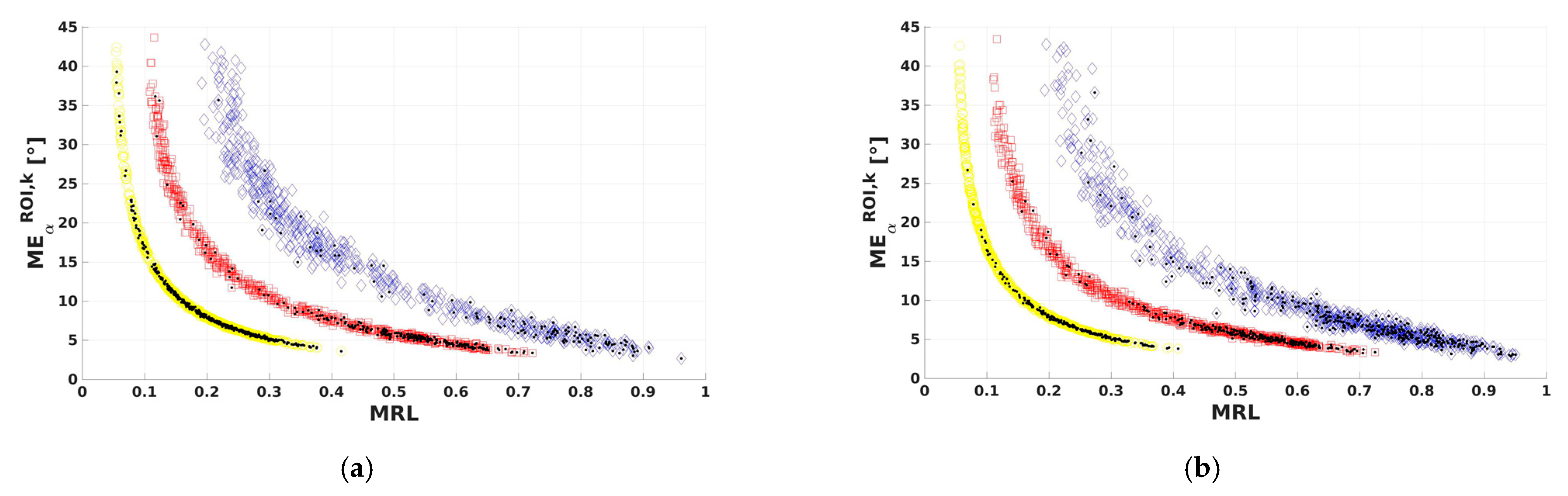
3.3. Exploitation of M E α R O I Aimed at Selection of the Optimal Local Processing Scale

The assessment of the MS LG-Mod at choosing the optimal local processing scale to reach the best directional estimation was evaluated on a dataset of 239 Sentinel-1 5 km by 5 km ROIs, as previously described.
Figure 10 reports the numbers of reliable directions (y-axis), respectively, as function of the applied threshold (x-axis). Moreover, for the Sentinel-1 ROIs dataset, the number of reliable directions obtained by the MS processing (i.e., N M u l t i T H w.r.t. population { R O I M u l t i T H } ) was greater than the one derived from each SS processing (i.e., N S i n g l e , k T H w.r.t. population { R O I S i n g l e , k T H } ). The MS processing provided a percentage improvement increasing from 3.48% to 23.74% w.r.t. the Low Scale, from 4.85% to 33.33% w.r.t. the Medium Scale, and from 6.73% to 129.33% w.r.t. the High Scale, while decreasing the threshold from 44.999° to 7.5°.
Figure 11a plots the RMSE values obtained from the MS and each SS processing (i.e., R M S E M u l t i and R M S E S i n g l e , k ) evaluated on the MS population of directions (i.e., { R O I M u l t i T H } ) and for each threshold value M E T H . The MS performance was proven to be better than the one from each SS processing, especially for higher threshold values M E T H , also exploiting real Sentinel-1 SAR data. From the RMSE values plotted in Figure 11a, the corresponding difference (i.e., R M S E M u l t i R M S E S i n g l e , k ), evaluated on the same MS population of directions (i.e., { R O I M u l t i T H } ), is obtained and reported in Figure 11b.
It can be noticed that, in general, the effect of the application of the threshold M E T H is that to reduce gradually RMSE values obtained, especially for M E T H lower than 15°. This is true for both MS and SS processing (Figure 11a). Applying the same M E T H , the MS procedure performs better than each SS one with an improvement of RMSE ranging from −2.23° (238) to −0.67° (172) w.r.t. the Low Scale, from −4.15° (238) to −1.80° (172) w.r.t. the Medium Scale, and from −10.52° (238) to −8.73° (172) w.r.t. the High Scale (Figure 11b). Number of estimates to which RMSE values refer are reported in brackets for each scale of comparison and for thresholds 44.999° and 7.5°, respectively (Figure 12).
Figure 13 plots the Mean Bias Error (MBE) values obtained from the MS and each SS processing (i.e., M B E M u l t i and M B E S i n g l e , k ) evaluated on the MS population of directions (i.e., { R O I M u l t i T H } ) and for each threshold value M E T H . It appears that both MS and SS directional estimations are biased with respect to the in situ measurements. The MBE values result positive, thus suggesting an overestimation of the wind directions derived from SAR data comparing with in situ data. The trends observed show an increasing of MBE values with a decreasing of the threshold M E T H . The MS directions generally result less biased (with MBE of about 1.2°) w.r.t. the ones derived from each SS processing, whereas the High Scale always presents a bias greater than the Medium Scale and, in turn, the Low Scale.
It is important to mention that MS wind direction improvement also yields to better wind speed retrieval through a GMF inversion. In fact, applying the C-band MODel 5.N (CMOD5.N) backscattering model [10], it was found that wind speed RMSE values are reduced up to −0.3 m/s using the wind direction derived from the MS processing rather than the one from each SS directional estimation.
Furthermore, previous analyses were also carried out on a ROI size of 12.5 km by 12.5 km. However, the number of available ROIs reduces up to 203. This reduction depends on the greater number of larger ROIs containing non-wind features and that are then discarded following the above-described procedure (Section 3.2). Moreover, in the case of NOAA stations located near the S-1 frames boundaries, it was not always allowed to extract 12.5 km by 12.5 km ROIs entirely included within the frames.
As reported in Figure 14, results obtained for the larger ROI size show the following:
(1)
The effectiveness in the application of the threshold M E T H is reduced, In fact, as shown in Figure 14a, the number of selected reliable directions decreases with the threshold less significantly than in the case of the ROI size of 5 km × 5 km (Figure 10). In addition, both RMSE and MBE trends, shown in Figure 14b,c, respectively, appear more flat with respect to the case of the smaller ROI size (Figure 11a and Figure 13, respectively). Thus, the 12.5 km by 12.5 km ROIs appear to have an associated directional content higher than the ones for the 5 km by 5 km case.
(2)
Both MS and SS directional estimations provide higher RMSE and (absolute) MBE values than the corresponding ones obtained at 5 km by 5 km ROI size. This can be justified considering that about half of the available in situ wind observations derived from stations with a maximum time distance from SAR acquisitions of 5 min, and the remaining measures does not exceed a 30 min delay. Moreover, the analysis is mainly performed in low–moderate wind speeds (i.e., up to 10 m/s).
(3)
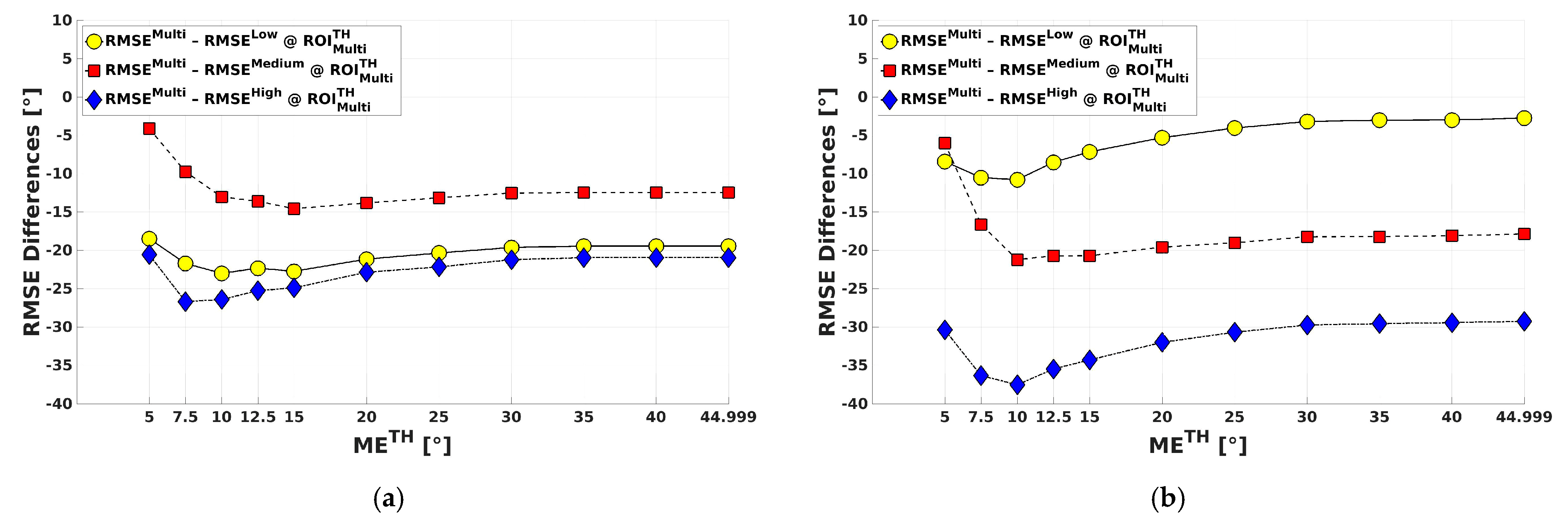
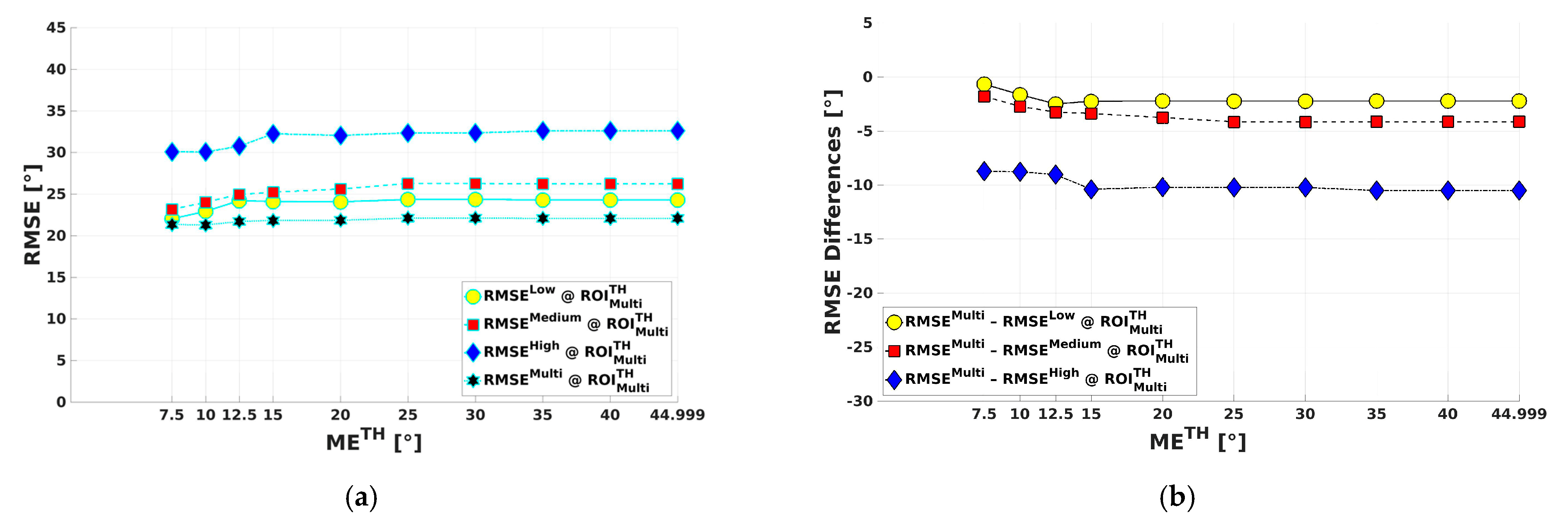
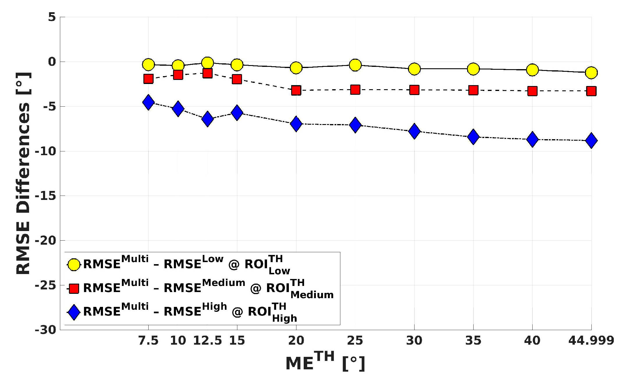
The MS estimation performance is still better than the one achieved by each SS processing, but the improvement reduces, especially in terms of achieved RMSE values with respect to the Low Scale. In fact, the improvement of RMSE reduces up to −0.09° w.r.t. the Low Scale, to −2.38° w.r.t. the Medium Scale, and to −7.25° w.r.t. the High Scale, whereas it reaches, with M E T H = 7.5 ° , about −2.23°, −4.15°, and −10.52°, respectively, for the 5 km by 5 km ROI size processing (Figure 11b).

3.4. Investigations on the Dependence of the Patterns Modulation Scale on Environmental Parameters

By exploiting wind data from NOAA in situ stations and related information (Table 1), some investigations were carried out in order to understand which physical phenomena may affect wind rows modulation scales, or—more precisely—processing scales locally selected as optimal by the MS LG-Mod.
It is worth noting that the following findings refer to directional estimations obtained by the MS LG-Mod on the Sentinel-1 5 km by 5 km ROIs selected, applying a final thresholding with M E T H = 15 ° and α = 0.05 as well. The latter threshold was chosen with the double aim to obtain reliable enough directional estimations and an acceptable number of 226 samples for statistical purpose.
The bar graph in Figure 15 shows the number of occurrences of the optimal processing scales (y-axis) for each one of the 17 NOAA stations (x-axis). The figure evidences the following:
  • The Low Scale (yellow) was the most frequently selected, i.e., 116 of the 226 occurrences (51.3%). The RMSE evaluated on these 116 occurrences was 21.38°.
  • The Medium Scale (red) was selected in 73 of the 226 occurrences (32.3%). The RMSE evaluated on the 73 occurrences was 21.44°.
  • The High Scale (blue) resulted the less frequent scale, i.e., 37 of the 226 occurrences (16.4%). The RMSE evaluated on the 37 occurrences was 22.33°.
A further analysis was suggested on the dependence of the wind rows modulation scale on both the distance from the coastline and the bathymetry for the available NOAA stations locations. Figure 16a,b displays, respectively, the bar graphs of the percentage of occurrences of the optimal processing scales (y-axes) grouped into three ranges of (a) distance from the coastline (near, 0 ≤ R< 10 km; mid, 10 km ≤ R < 20 km; far, R ≥ 20 km) and (b) bathymetry (low, 0 ≤ Z < 75 m; moderate, 75 m ≤ Z < 150 m; high, Z > 150 m) (x-axes). The former ranges are quite uniformly covered, with the 34.9%, the 34.9%, and the 30.2% of samples in the near, mid, and far range, respectively. Most of the in situ stations are located at low (57.9%) and moderate (33.2%) bathymetry, while just a small percentage of stations (8.8%) is characterized by high values of bathymetry. The following points were observed:
  • The percentage of occurrences of the Low- and the Medium-Scale selection reduces and increases, respectively, while the distance R from the coastline is increasing. On the other hand, the High-Scale selection presents about the same percentage of occurrences in the three range of distance.
  • The Low- and the Medium-Scale selections do not show a well-defined relationship between the percentage of occurrences and the bathymetry Z. Instead, the frequency of the High-Scale selection increases with the bathymetry.
The dependence of the wind rows modulation scale on both wind speed and direction as measured by NOAA in situ stations was also examined. Figure 17a,b shows, respectively, the bar graphs of the percentage of occurrences of the optimal processing scales (y-axes) grouped into three ranges of wind (a) speed (light: 2 ≤ W < 5.5 m/s; moderate: 5.5 ≤ W < 13.8 m/s; Strong: W > 13.8 m/s) and (b) direction (on-shore and off-shore notations refer to winds that go from the sea toward the land and vice versa respectively; along-shore means winds that blow almost parallel to the coast) (x-axes). Most of the in situ wind observations show a moderate (the 67.7% of the total amount) wind speed regime, while the remaining observations are in the light (31.4%) and strong (0.9%) range of wind. Wind rows were detected almost exclusively in the light and moderate wind-speed regimes. In particular, the range of moderate wind speeds, from 5.5 to 13.8 m/s, seems to be the most suitable to allow visibility of wind rows on SAR images. Concerning the actual in situ wind directions, available observations are in the off-shore, along-shore, and on-shore ranges with the percentage of occurrences of the 25.7%, the 67.7%, and the 6.6%, respectively. Wind rows were detected mostly in case of along-shore winds rather than off- and on-shore winds. The following points were observed:
  • From Figure 17a, the percentage of occurrences of the Low- and the Medium-Scale selection reduces and increases, respectively, while the wind speed is increasing from the light to the moderate regimes. The High-Scale selection presents about the same percentage of occurrences in both regimes. The Strong case is poorly sampled, and it may be only stated that strong wind speeds were proven to be a bad condition for wind rows visibility.
  • From Figure 17b, the Low-, the Medium-, and the High-Scale selections do not show a well-defined relationship between the percentage of occurrences and the wind direction range.
Unfortunately, in situ measurements of air and sea temperature were only partially available. For this reason, it was not possible to extend the same previous analysis to these variables, although these types of information are important for boundary layer roll and wind streak development.
Two Sentinel-1 IW images are shown in Figure 18 as NRCS values with superimposed wind directions retrieved by the MS LG-Mod (with M E T H = 10 ° and α = 0.05 ). SSW directions were estimated by the algorithm over a grid of about 0.05° by 0.05° (latitude by longitude). Three processing scales, i.e., the High Scale (320 m by 320 m, blue), the Medium Scale (160 m by 160 m, red), and the Low Scale (80 m by 80 m, yellow) were exploited with the aim at spanning the pixel size range (100–400 m) for wind rows detection. According to the DAMC, each different color represents the scale that is locally regarded as optimal by the MS LG-Mod.
The continental-scale Rapid Refresh (RAP) NWP model was used to solve the 180° ambiguity in the SAR wind directions retrieval. RAP assimilation/modeling system covers North America (N: 59.0°, S: 16.2°, E: −57.3°, W: −139.9°) and provides daily hourly updated analysis data on a resampled UTM (Universal Transverse Mercator) 13 km resolution horizontal grid (dataset: Rapid Refresh (RAP) [13 km], NCEI DSI 6187_08).
The full frame analysis highlights that the Low Scale (80 m by 80 m, yellow) was the most frequently selected while the other scales were especially found in the coastal areas characterized by moderate bathymetry. These findings partially confirm what was found in the analysis made by using buoys data.

4. Discussion

4.1. LG-Mod Results from Simulated SAR Images

As pointed out by Figure 5a,b, the adoption of the DAMC criterion allows the MS LG-Mod algorithm to locally choose the processing scale that may be regarded as optimal for patterns enhancement. This scale is clearly correlated on the varying spatial wavelength of the local patterns.
As shown in Figure 6a,b, the same DAMC criterion guarantees, as expected, the maximum number of reliable directions selected by the MS LG-Mod in comparison with those obtained by each SS processing, when the same threshold of acceptance M E T H is applied.
Moreover, the MS LG-Mod optimal scale selection provides the best choice for local directional estimation depending on the set of previously fixed processing scales. This statement is confirmed by the plots in Figure 7 and Figure 8, from which the RMSE value derived from MS LG-Mod directional estimates is always lower than those values obtained from SS LG-Mod ones. This finding is true considering both MS and SS populations of reliable directions obtained from each applied threshold M E T H .
However, it is worth noting that the lower the threshold the better each SS directional estimation, according to the fact that RMSE differences tend progressively to zero for decreasing values of the threshold M E T H (Figure 8). This evidence suggests the idea that SS directional populations become mutually exclusive when the applied threshold M E T H is very low (Figure 6). On the contrary, when the latter constrain is not very strict (i.e., higher threshold), an overlap of SS populations may occur and the MS analysis thus supports the optimal processing scale selection among the different SS employed ones.

4.2. LG-Mod Results from Real SAR Images

As detailed in Reference [17], for the SS LG-Mod algorithm, the Marginal Error M E α R O I is a function of the scalar Mean Resultant Length (MRL), which represents a measure of a ROI local directions alignment. It follows that the parameter M E α R O I indirectly provides directional content of a ROI. The smaller the Marginal Error, as well as the better the accuracy of the directional estimate, the higher the ROI directional content. This is also true within the framework of the novel MS LG-Mod.
Hence, M E α R O I is capable of detecting wind rows patterns by means of their directional content estimation only in the case of an effective removal of artifacts and non-wind features onto SAR images. Otherwise, the directional content sensed by the parameter M E α R O I would be obviously not related to the local wind direction to be estimated. As a consequence, such conditions need to be avoided, e.g., as implemented by the above described strategy (Section 3.2).

4.3. Exploitation of M E α R O I Aimed at Selection of the Optimal Local Processing Scale

Statistics plotted in Figure 10, Figure 11 and Figure 12 obtained on the Sentinel-1 ROIs selection clearly confirm results achieved for simulated SAR images. This finding supports the fact that, in the case of artifacts and non-wind features removal from real SAR images, the M E α R O I parameter and the DAMC criterion—defined within the MS LG-Mod—guarantee the automatic selection of the optimal local processing scale for the best achievable local direction estimation. In such case, the novel MS analysis proved to be able to sense local directional content better than each SS processing. The MS directional analysis also leads to an improvement in SAR wind speed retrieval, although the found minimal impact on this retrieval (the maximum RMSE difference is of about −0.3 m/s) may be caused by the actual low to moderate wind conditions of the S-1 dataset.
Even though in Reference [28] and in Reference [30] frequencies of modulations belonging to the BLRs and WSs are enhanced, no effective selection of optimal scale is performed within these two methods.
The two approaches proposed in Reference [32], to choose the optimal estimated direction are based either on the use of a priori information from a NWP model or the visual inspection of patterns visible on SAR amplitude. The first option makes the LG method dependent on external data, which could be not sufficiently accurate. The second one makes the method itself not completely automated.
The criterion proposed in Reference [17], which defines the optimal processing scale as the one which can globally yield in a single SAR the largest percentage of reliable ROIs, gave promising results. However, the different mechanisms that may induce wind aligned streaks on SAR images produce SAR NRCS modulations with wavelengths ranging from few hundred meters to few kilometers [22], which may occur even in the same SAR image. This may hamper the use of a criterion previously described in Reference [17].
In Reference [27] the computation of a directional factor at different scales was proposed to find the optimal scale. The scale with the highest value of that parameter gives the optimal scale of the directional feature. To the best of our knowledge, this is the only attempt to find the local optimal scale by means of an automatic criterion. Nonetheless, no quantitative comparison was made between the performance of the single- and multiple-scale algorithms.
In the present work, a local MS criterion for the optimal pixel size (scale) automatic selection was introduced and it was proved to perform better with respect to the use of a SS one, especially at high-resolution (i.e., 5 km by 5 km ROI size) processing.

4.4. Investigations on the Dependence of the Patterns Modulation Scale on Environmental Parameters

The results reported in Section 3.4 revealed that wind rows modulation scales may be determined by several concurring factors, such as distance from the coast, bathymetry and wind characteristics as well. The following points are offered to summarize the results:
  • The Low (80 m × 80 m) and the Medium (160 m × 160 m) Scales represent the more adequate ones for wind rows detection, as shown by both the frequency of occurrences (i.e., 51.3% and 32.3%, respectively) and the accuracy of directional estimations (i.e., RMSE values equal to 21.38° and 21.44°, respectively). Furthermore, both scales may occur at different distances from the coast, but it is not clear why the frequency of the Low- and Medium-Scale selection decreases and increases, respectively, while the distance from the cost increases (Figure 17a). A possible interpretation is that wind-induced SAR signatures, namely wind rows, may be affected close to the coast by a mixing of different modulations due to both Wind Streaks and Boundary Layer Rolls. The former are typically characterized by spatial wavelengths that are more compatible with the Low Scale, whereas the latter are more detectable with the Medium Scale.
  • The High Scale (320 m × 320 m) resulted in being, instead, the less frequent, as well as the less accurate, scale employed, with a percentage of occurrences and a RMSE equal to 16.4% and 22.33°, respectively (Figure 12). This scale seems to be just influenced by the bathymetry, showing an increasing of percentage of occurrences with the bathymetry itself (Figure 16b). To the best of our knowledge, no authors have been investigated on the effects of the bathymetry on SAR backscattering modulations induced by atmospheric phenomena, such as wind rows. However, it is well-known that, in shallow areas, small-scale features of the bathymetry cause strong current gradients, which then in turn modulate the spectrum of the short Bragg waves [39]. Zhang et al., in 2017, found different bathymetric features on SAR imagery under different sea states. In particular, under low to moderate wind speeds (3.1~6.3 m/s), they observed wide bright patterns with an average width of 6 km and quasi-linear features only 1 km wide for high winds (5.4~13.9 m/s) [40]. On the other hand, it is recognized that the approximation of waves to shallow areas results in a decrease in the wavelength, which is linked to water depths [41]. However, although wind rows derived modulations in the SAR image are primarily caused by variations in the near-surface wind field, the bathymetry may change their spatial wavelengths, as suggested by the increasing of percentage of High-Scale occurrences with the bathymetry.
  • Wind rows are detected mostly in the case of light–moderate wind speed regimes (i.e., W less than 13.8 m/s) and along-shore winds (Figure 17a,b, respectively). This finding confirms the results in References [20,21], where it is reported that wind rows are most commonly observed at wind speeds near 8–9 m/s. Whatever the wind speed and direction, the Low- and the Medium-Scale selections occur more frequently than the High-Scale one.
  • However, the wind rows modulation scale may be also influenced by any further physical phenomena that cause variations of the sea surface roughness and, in turn, the radar signal backscattered from the sea. As reported in Reference [18], there is a large variability in wavelength and amplitude of the wind rows as a result of several processes acting on the wind rows and related to the inhomogeneities in terrain, roughness, and heating and also to vertical wind shear [42].

5. Conclusions

A novel MS analysis was introduced and fully developed within the LG-Mod algorithm [8,17] with the aim to improve the reliability of SAR-derived SSW directions retrieval.
The MS LG-Mod was proven to be able to automatically select the optimal local processing scale for wind patterns enhancement in order to provide the best achievable local directional estimation, once a set of processing scales has been fixed.
The assessment of the MS LG-Mod directional estimation was carried out on both simulated SAR data and Sentinel-1 images.
Results achieved from simulated SAR images showed that the MS analysis allows to sense local directional content better than each SS processing. In fact, the MS LG-Mod evidenced to locally choose the processing scale that is optimal for patterns enhancement and clearly correlated on the spatial wavelength of the local patterns.
The MS procedure performed always better than each SS one, with improvements in terms of both directional RMSE values and percentages of reliable output directions achieved.
For the analysis of the S-1 dataset, the removal of artifacts and non-wind features from SAR amplitudes was mandatory before directional estimations. Hence, the application of the MS LG-Mod algorithm always requires taking into account the removal of such features.
Further developments should lead to completely automate this step.
Finally, a tentative analysis on the dependence of the patterns modulation scale on environmental parameters was made. The Low (80 m × 80 m) and the Medium (160 m × 160 m) Scales resulted the more adequate ones for wind rows detection on Sentinel-1 data, as evidenced by both their frequency of occurrence and the accuracy of directional estimation. The High Scale (320 m × 320 m) was instead the less frequent and accurate scale employed.
Hence, the analysis revealed that both the Low and the Medium Scales may occur at different distances from the coast, showing a frequency of the Low- and Medium-Scale selection that decreases and increases, respectively, with the distance from the cost itself. Moreover, wind rows were detected mostly in light–moderate wind speed regimes and for along-shore winds, for the examined coastal dataset. However, wind rows visibility and their modulation scales may be determined by several concurring physical parameters, which cause variations of the sea surface roughness. That is the reason to further investigate, e.g., using the full-frame analysis only introduced in this work.

Author Contributions

Conceptualization, F.M.R. and M.A.; Data curation, F.M.R. and M.A.; Formal analysis, F.M.R.; Investigation, F.M.R. and M.A.; Methodology, F.M.R.; Resources, F.M.R. and M.A.; Software, F.M.R.; Supervision, F.M.R. and M.A.; Validation, F.M.R. and M.A.; Visualization, F.M.R.; Writing—original draft, F.M.R.; Writing—review & editing, F.M.R. and M.A.. All authors have read and agreed to the published version of the manuscript.

Funding

This work was supported by the European Union’s Horizon2020 research and innovation program, within the projects GEOEssential, ERA-NET-Cofund Grant, Grant Agreement No. 689443 and E-SHAPE—myEcosystem showcase, Grant Agreement ID 820852.

Institutional Review Board Statement

Not applicable.

Informed Consent Statement

Not applicable.

Data Availability Statement

Data sharing not yet available.

Acknowledgments

The authors would like to thank Palma Blonda for supporting this study in terms of project administration and funding acquisition.

Conflicts of Interest

The authors declare no conflict of interest. The funders had no role in the design of the study; in the collection, analyses, or interpretation of data; in the writing of the manuscript; or in the decision to publish the results.

References

  1. Villas Boas, A.B.; Ardhuin, F.; Ayet, A.; Bourassa, M.A.; Chapron, B.; Brandt, P.; Gille, S.T. Integrated observations and modeling of global winds, currents, and waves: Requirements and challenges for the next decade. Front. Mar. Sci. 2019, 6, 425. [Google Scholar] [CrossRef]
  2. Borrelli, P.; Lugato, E.; Montanarella, L.; Panagos, P. A new assessment of soil loss due to wind erosion in European agricultural soils using a quantitative spatially distributed modelling approach. Land Degrad. Dev. 2017, 28, 335–344. [Google Scholar] [CrossRef] [Green Version]
  3. Nezhad, M.M.; Groppi, D.; Marzialetti, P.; Fusilli, L.; Laneve, G.; Cumo, F.; Garcia, D.A. Wind energy potential analysis using Sentinel-1 satellite: A review and a case study on Mediterranean islands. Renew. Sustain. Energy Rev. 2019, 109, 499–513. [Google Scholar] [CrossRef]
  4. Mouche, A.A.; Collard, F.; Chapron, B.; Dagestad, K.F.; Guitton, G.; Johannessen, J.A.; Hansen, M.W. On the use of Doppler shift for sea surface wind retrieval from SAR. IEEE Trans. Geosci. Remote Sens. 2012, 50, 2901–2909. [Google Scholar] [CrossRef]
  5. Zhang, B.; Perrie, W.; Vachon, P.W.; Li, X.; Pichel, W.G.; Guo, J.; He, Y. Ocean vector winds retrieval from C-band fully polarimetric SAR measurements. IEEE Trans. Geosci. Remote Sens. 2012, 50, 4252–4261. [Google Scholar] [CrossRef] [Green Version]
  6. Benassai, G.; Migliaccio, M.; Nunziata, F. The use of COSMO-SkyMed© SAR data for coastal management. J. Mar. Sci. Technol. 2015, 20, 542–550. [Google Scholar] [CrossRef]
  7. Komarov, A.S.; Zabeline, V.; Barber, D.G. Ocean surface wind speed retrieval from C-band SAR images without wind direction input. IEEE Trans. Geosci. Remote Sens. 2013, 52, 980–990. [Google Scholar] [CrossRef]
  8. Rana, F.M.; Adamo, M.; Blonda, P. LG-mod multi-scale approach for SAR sea surface wind directions retrieval. In Proceedings of the IEEE International Geoscience and Remote Sensing Symposium (IGARSS), Valencia, Spain, 22–27 July 2018. [Google Scholar]
  9. Radkani, N.; Zakeri, B.G. Sea Wind Retrieval by Analytically-Based Geophysical Model Functions and Sentinel-1A SAR Images. Prog. Electromagn. Res. 2019, 93, 223–236. [Google Scholar] [CrossRef] [Green Version]
  10. Hersbach, H. Comparison of C-band scatterometer CMOD5. N equivalent neutral winds with ECMWF. J. Atmos. Ocean. Technol. 2010, 27, 721–736. [Google Scholar] [CrossRef]
  11. Stoffelen, A.; Verspeek, J.A.; Vogelzang, J.; Verhoef, A. The CMOD7 geophysical model function for ASCAT and ERS wind retrievals. IEEE J. Sel. Top. Appl. Earth Obs. Remote Sens. 2017, 10, 2123–2134. [Google Scholar] [CrossRef]
  12. Li, X.M.; Lehner, S. Algorithm for sea surface wind retrieval from TerraSAR-X and TanDEM-X data. IEEE Trans. Geosci. Remote Sens. 2013, 52, 2928–2939. [Google Scholar] [CrossRef] [Green Version]
  13. La, T.V.; Khenchaf, A.; Comblet, F.; Nahum, C. Exploitation of C-band Sentinel-1 images for high-resolution wind field retrieval in coastal zones (Iroise coast, France). IEEE J. Sel. Top. Appl. Earth Obs. Remote Sens. 2017, 10, 5458–5471. [Google Scholar] [CrossRef]
  14. Mouche, A. Sentinel-1 ocean wind fields (OWI) algorithm definition. In Sentinel-1 IPF Reference: (S1-TN-CLS-52-9049) Report; CLS: Brest, France, 2010; pp. 1–75. [Google Scholar]
  15. Monaldo, F.; Jackson, C.; Li, X.; Pichel, W.G. Preliminary evaluation of Sentinel-1A wind speed retrievals. IEEE J. Sel. Top. Appl. Earth Obs. Remote Sens. 2016, 9, 2638–2642. [Google Scholar] [CrossRef]
  16. Ahsbahs, T.; Badger, M.; Karagali, I.; Larsén, X.G. Validation of Sentinel-1A SAR coastal wind speeds against scanning LiDAR. Remote Sens. 2017, 9, 552. [Google Scholar] [CrossRef] [Green Version]
  17. Rana, F.M.; Adamo, M.; Lucas, R.; Blonda, P. Sea surface wind retrieval in coastal areas by means of Sentinel-1 and numerical weather prediction model data. Remote Sens. Environ. 2019, 225, 379–391. [Google Scholar] [CrossRef]
  18. Svensson, N.; Sahlée, E.; Bergström, H.; Nilsson, E.; Badger, M.; Rutgersson, A. A case study of offshore advection of boundary layer rolls over a stably stratified sea surface. Adv. Meteorol. 2017, 2017, 9015891. [Google Scholar] [CrossRef] [Green Version]
  19. Dankert, H.; Horstmann, J.; Rosenthal, W. Ocean wind fields retrieved from radar-image sequences. J. Geophys. Res. Oceans 2003, 108, 1–11. [Google Scholar] [CrossRef]
  20. Zhao, Y.; Li, X.M.; Sha, J. Sea surface wind streaks in spaceborne synthetic aperture radar imagery. J. Geophys. Res. Oceans 2016, 121, 6731–6741. [Google Scholar] [CrossRef]
  21. Wang, C.; Vandemark, D.; Mouche, A.; Chapron, B.; Li, H.; Foster, R.C. An assessment of marine atmospheric boundary layer roll detection using Sentinel-1 SAR data. Remote Sens. Environ. 2020, 250, 112031. [Google Scholar] [CrossRef]
  22. Koch, W. Directional analysis of SAR images aiming at wind direction. IEEE Trans. Geosci. Remote Sens. 2004, 42, 702–710. [Google Scholar] [CrossRef]
  23. Fetterer, F.; Gineris, D.; Wackerman, C.C. Validating a scatterometer wind algorithm for ERS-1 SAR. IEEE Trans. Geosci. Remote Sens. 1998, 36, 479–492. [Google Scholar] [CrossRef]
  24. Zhou, L.; Zheng, G.; Li, X.; Yang, J.; Ren, L.; Chen, P.; Zhang, H.; Lou, X. An improved local gradient method for sea surface wind direction retrieval from SAR imagery. Remote Sens. 2017, 9, 671. [Google Scholar] [CrossRef] [Green Version]
  25. Zecchetto, S.; De Biasio, F. A wavelet-based technique for sea wind extraction from SAR images. IEEE Trans. Geosci. Remote Sens. 2008, 46, 2983–2989. [Google Scholar] [CrossRef]
  26. Zheng, G.; Li, X.; Zhou, L.; Yang, J.; Ren, L.; Chen, P.; Zhang, H.; Lou, X. Development of a gray-level co-occurrence matrix-based texture orientation estimation method and its application in sea surface wind direction retrieval from SAR imagery. IEEE Trans. Geosci. Remote Sens. 2018, 56, 5244–5260. [Google Scholar] [CrossRef]
  27. Du, Y.; Vachon, P.W.; Wolfe, J. Wind direction estimation from SAR images of the ocean using wavelet analysis. Can. J. Remote Sens. 2002, 28, 498–509. [Google Scholar] [CrossRef]
  28. Leite, G.C.; Ushizima, D.M.; Medeiros, F.N.; De Lima, G.G. Wavelet analysis for wind fields estimation. Sensors 2010, 10, 5994–6016. [Google Scholar] [CrossRef] [Green Version]
  29. Noratiqah, M.D.S.; Arnis, A.; Shattri, M. Modification of wavelet transform approach for low-wind direction extraction. In Proceedings of the IEEE International Conference on Aerospace Electronics and Remote Sensing Technology (ICARES), Bali, Indonesia, 3–5 December 2015. [Google Scholar]
  30. Zecchetto, S. Wind Direction Extraction from SAR in Coastal Areas. Remote Sens. 2018, 10, 261. [Google Scholar] [CrossRef] [Green Version]
  31. Farahani, F.T.; Keshavarz, A.; Zecchetto, S. Wind Direction Extraction from Sar Images Using Nsct Transform. In Proceedings of the IEEE International Geoscience and Remote Sensing Symposium (IGARSS), Valencia, Spain, 22–27 July 2018. [Google Scholar]
  32. Koch, W.; Feser, F. Relationship between SAR-derived wind vectors and wind at 10-m height represented by a mesoscale model. Mon. Weather Rev. 2006, 134, 1505–1517. [Google Scholar] [CrossRef] [Green Version]
  33. Fisher, N.I.; Lewis, T. Estimating the common mean direction of several circular or spherical distributions with differing dispersions. Biometrika 1983, 70, 333–341. [Google Scholar] [CrossRef]
  34. Rana, F.M.; Adamo, M.; Pasquariello, G.; De Carolis, G.; Morelli, S. LG-Mod: A modified local gradient (LG) method to retrieve SAR sea surface wind directions in marine coastal areas. J. Sens. 2016, 2016, 9565208. [Google Scholar] [CrossRef] [Green Version]
  35. Trivero, P.; Biamino, W. Observing marine pollution with Synthetic Aperture Radar. In Geoscience and Remote Sensing New Achievements; InTech Open: London, UK, 2010; pp. 397–418. [Google Scholar]
  36. Santamaria, C.; Alvarez, M.; Greidanus, H.; Syrris, V.; Soille, P.; Argentieri, P. Mass processing of sentinel-1 images for maritime surveillance. Remote Sens. 2017, 9, 678. [Google Scholar] [CrossRef] [Green Version]
  37. Topouzelis, K.; Kitsiou, D. Detection and classification of mesoscale atmospheric phenomena above sea in SAR imagery. Remote Sens. Environ. 2015, 160, 263–272. [Google Scholar] [CrossRef]
  38. Sikora, T.D.; Young, G.S.; Beal, R.C.; Monaldo, F.M.; Vachon, P.W. Applications of synthetic aperture radar in marine meteorology. In Atmosphere Ocean Interactions; Perrie, W., Ed.; WIT Press: Southampton, UK, 2006; Volume 2, pp. 83–105. [Google Scholar]
  39. Müller, S.; Stanev, E.V.; Schulz-Stellenfleth, S.; Staneva, J.; Koch, W. Atmospheric boundary layer rolls: Quantification of their effect on the hydrodynamics in the German Bight. J. Geophys. Res. 2013, 118, 5036–5053. [Google Scholar] [CrossRef] [Green Version]
  40. Zhang, S.; Xu, Q.; Zheng, Q.; Li, X. Mechanisms of SAR Imaging of Shallow Water Topography of the Subei Bank. Remote Sens. 2017, 9, 1203. [Google Scholar] [CrossRef] [Green Version]
  41. Santos, D.; Abreu, T.; Silva, P.A.; Baptista, P. Estimation of Coastal Bathymetry Using Wavelets. J. Mar. Sci. Eng. 2020, 8, 772. [Google Scholar] [CrossRef]
  42. Wang, S.; Jiang, Q. Impact of vertical wind shear on roll structure in idealized hurricane boundary layers. Atmos. Chem. Phys. 2017, 17, 3507–3524. [Google Scholar] [CrossRef] [Green Version]
Figure 1. Simulated Synthetic Aperture Radar (SAR) images. Linear patterns (a) without and (c) with multiplicative speckle noise. Circular patterns (b) without and (d) with multiplicative speckle noise.
Remotesensing 13 00410 g001
Figure 2. Gulf of Maine (Northeastern America), showing the deployment of National Oceanic and Atmospheric Administration National Data Buoy Center (NOAA NDBC) wind-measurement stations (yellow and black-dotted icons). Sentinel-1 (S-1) full-frame coverage is in orange and cyan for descending (i.e., S1B-10391-40-1/2) and ascending (i.e., S1A-21484-62-1/2/5/6, S1B-10515-164-6, S1A-6740-18-1, S1A-15417-120-5, and S1A-7513-91-1) S-1 Interferometric Wide Swath Ground Range Multi-Look Detected High-Resolution (IW) images, respectively. Background image (Data SIO, NOAA, US Navy, NGA, GEBCO; Image Landsat/Copernicus) is from Google Earth.
Remotesensing 13 00410 g002
Figure 3. Multi-Scale Local-Gradient-Modified (MS LG-Mod) processing flowchart.
Remotesensing 13 00410 g003
Figure 4. Trends of Marginal Errors, i.e., the Single-Scale (SS) M E α R O I , k with k { 1 , , 3 } (colored markers) and the MS M E α R O I (black dots) values, as functions of the concentration parameter Mean Resultant Length (MRL), from noisy (a) linear and (b) circular patterns in Figure 1c,d respectively.
Remotesensing 13 00410 g004
Figure 5. (a,b) MS and (ch) SS LG-Mod directions estimated from (a,c,e,g) linear and (b,d,f,h) circular patterns in Figure 1c,d, respectively. Same final thresholding applied for each processing ( M E T H = 10 ° and α = 0.05 ). Yellow, red, and blue indicate the 80 m × 80 m (Low Scale), 160 m × 160 m (Medium Scale) and 320 m × 320 m (High Scale) processing scales.
Remotesensing 13 00410 g005aRemotesensing 13 00410 g005b
Figure 6. Percentages of reliable directions obtained by MS and SS processing ( P M u l t i T H and P S i n g l e , k T H , respectively) evaluated on each own population ( { R O I M u l t i T H } and { R O I S i n g l e , k T H } , respectively), plotted as function of the same applied threshold M E T H , for noisy (a) linear and (b) circular patterns in Figure 1c,d.
Remotesensing 13 00410 g006
Figure 7. R M S E M u l t i   R M S E S i n g l e , k evaluated on the multi-scale population { R O I M u l t i T H } , plotted as function of the applied threshold M E T H , for noisy (a) linear and (b) circular patterns in Figure 1c,d.
Remotesensing 13 00410 g007
Figure 8. R M S E M u l t i R M S E S i n g l e , k evaluated on the single-scale populations { R O I S i n g l e , k T H } , plotted as function of the applied threshold M E T H , for noisy (a) linear and (b) circular patterns in Figure 1c,d.
Remotesensing 13 00410 g008
Figure 9. Examples of some artifacts or non-wind features affecting S-1 ROIs amplitude: (a) spikes/bright areas, (b) radiofrequency interference, (c) dark areas, (d) atmospheric gravity waves, and (e) atmospheric convective cells. ROIs have 188 by 188 (azimuth by range) dimension, with a pixel size of 80 m by 80 m. They cover an area of about 15 km by 15 km.
Remotesensing 13 00410 g009aRemotesensing 13 00410 g009b
Figure 10. Number of reliable directions obtained by MS and SS processing ( N M u l t i T H and N S i n g l e , k T H , respectively), evaluated on each own population ( { R O I M u l t i T H } and { R O I S i n g l e , k T H } , respectively), plotted as function of the applied threshold M E T H . Dataset: Sentinel-1 5 km × 5 km ROIs selected. Reference wind directions from NOAA NDBC.
Remotesensing 13 00410 g010
Figure 11. (a) R M S E M u l t i and R M S E S i n g l e , k and (b) R M S E M u l t i   R M S E S i n g l e , k evaluated on MS population { R O I M u l t i T H } , plotted as function of the applied threshold M E T H . Dataset: Sentinel-1 5 km × 5 km ROIs selected. Reference wind directions from NOAA NDBC.
Remotesensing 13 00410 g011
Figure 12. R M S E M u l t i   R M S E S i n g l e , k , evaluated on each single-scale population { R O I S i n g l e , k T H } , plotted as function of the applied threshold M E T H . Dataset: Sentinel-1 5 km × 5 km ROIs selected. Reference wind directions from NOAA NDBC.
Remotesensing 13 00410 g012
Figure 13. M B E M u l t i and M B E S i n g l e , k evaluated on MS population { R O I M u l t i T H } , plotted as function of the applied threshold M E T H . Dataset: Sentinel-1 5 km × 5 km ROIs selected. Reference wind directions from NOAA NDBC.
Remotesensing 13 00410 g013
Figure 14. (a) Number of reliable directions obtained by MS and SS processing ( N M u l t i T H and N S i n g l e , k T H , respectively), evaluated on each own population ( { R O I M u l t i T H } and { R O I S i n g l e , k T H } , respectively); (b) R M S E M u l t i and R M S E S i n g l e , k , (c) M B E M u l t i and M B E S i n g l e , k evaluated on MS population { R O I M u l t i T H } . Plots are functions of the applied threshold M E T H . Dataset: Sentinel-1 12.5 km × 12.5 km ROIs selected. Reference wind directions from NOAA NDBC.
Remotesensing 13 00410 g014
Figure 15. Bar graph displaying the number of occurrences of the optimal processing scales (y-axis) corresponding to each available NOAA station (x-axis). Dataset: Sentinel-1 5 km × 5 km ROIs selected. Final thresholding: M E T H = 15 ° and α = 0.05 .
Remotesensing 13 00410 g015
Figure 16. Bar graph displaying the percentage of occurrences of the optimal processing scales (y-axes) grouped by (a) distance from the coastline and (b) bathymetry (x-axes). Dataset: Sentinel-1 5 km × 5 km ROIs selected. Final thresholding: M E T H = 15 ° and α = 0.05 .
Remotesensing 13 00410 g016
Figure 17. Bar graph displaying the percentage of occurrences of the optimal processing scales (y-axis) grouped by wind (a) speed and (b) direction (x-axis). Dataset: Sentinel-1 5 km × 5 km ROIs selected Final thresholding: M E T H = 15 ° and α = 0.05 .
Remotesensing 13 00410 g017
Figure 18. MS LG-Mod wind directions, estimated over a grid of about 0.05° by 0.05° (latitude by longitude), for two S-1 IW images (Gulf of Maine) with VV-polarizations, along ascending orbit, on (a) the 29 August 2015 and (b) the 10 October 2016. Final thresholding applied with M E T H = 5 ° (and α = 0.05 ). Blue, red, and yellow indicate the 320 m × 320 m (High Scale), 160 m × 160 m (Medium Scale), and 80 m × 80 m (Low Scale) processing scales, respectively. Unusable pixels are in green.
Remotesensing 13 00410 g018
Table 1. Information about NOAA NDBC in situ stations.
NOAA
Station
ID
Longitude (°)Latitude (°)Temporal Resolution
(min)
Direction
Accuracy (°)
Distance from Coastline (km)Bathymetry (m)
44005−69.12843.20160180177.0
44007−70.14143.525601728.8
44011−66.61941.09860128385.3
44013−70.65142.3466011462.9
44018−70.14342.2066012943.2
44020−70.27941.4936011211.4
44027−67.30744.28360127185.3
44029−70.56642.523100.1964.5
44030−70.42643.179100.11369.1
44032−69.35543.716100.11885.6
44033−68.99844.055100.15104.2
44034−68.11244.103100.12197.0
44037−67.87943.491100.185277.6
MDRM1−68.12843.9696012854.8
MISM1−68.85543.7846013331.2
44137−62.00042.266012952962.2
44150−64.0242.56011561301.8
Publisher’s Note: MDPI stays neutral with regard to jurisdictional claims in published maps and institutional affiliations.

