Monitoring 2019 Forest Fires in Southeastern Australia with GNSS Technique


Abstract
1. Introduction
2. Materials and Methods
2.1. Materials
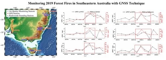
2.1.1. Study Area
2.1.2. Data
2.2. Methodology
2.2.1. PWV Inversion Based on GNSS Data
2.2.2. PWV Inversion Based on Radiosonde Data
2.2.3. Monitoring Forest Fires with ΔPWV
3. Result and Analysis
3.1. Correlation between PM2.5 and PM10
3.2. Analysis of Forest Fire Monitoring in Southeastern Australia Based on GNSS
3.3. Correlation Analysis of ΔPWV and PM10
4. Discussion
5. Conclusions
- (1)
- In climate conditions with regular precipitation, such as Mediterranean climate and temperate marine climate, it is feasible to use ΔPWV to monitor forest fires. The performance is very stable before and during the fire. After the fire, it is impossible to monitor the forest fire due to particulate matter stagnation in the air.
- (2)
- In climatic conditions with irregular precipitation, such as humid subtropical climate, due to more precipitation in the rainy season and strong transpiration caused by temperature rise, ΔPWV will be severely affected.
- (3)
- When the fire occurs, much PM10 will be produced, and the correlation between ΔPWV and PM10 will increase. Therefore, ΔPWV can be used to study the pollution caused by PM10/PM2.5 from fire. After the fire, ΔPWV can also reflect the stagnation of particulate matter, so ΔPWV can be used to study particulate matter stagnation in the environment in future work.
- (4)
- ΔPWV will be affected by climate, precipitation, wind direction, and other environment factors, which demonstrates that monitoring forest fires needs further research in climate conditions with irregular precipitation using GNSS technique.
Author Contributions
Funding
Informed Consent Statement
Data Availability Statement
Acknowledgments
Conflicts of Interest
References
- Adams, M.A.; Shadmanroodposhti, M.; Neumann, M. Causes and consequences of Eastern Australia’s 2019–20 season of mega-fires: A broader perspective. Glob. Change Biol. 2020, 26, 3756–3758. [Google Scholar] [CrossRef]
- Proloy, D.; Hamid, M.; Peyman, A.; Anthony, S.K.; Johanna, E.; David, K.; Ashish, S. Causes of the Widespread 2019–2020 Australian Bushfire Season. Earth’s Future 2020, 8, e2020EF001671. [Google Scholar]
- O’Loughlin, C.; Jones, S.C.; Jenkins, M.; Gordon, C.E. The effects of inter-fire interval on flora-fauna interactions in a sub-alpine landscape. For. Ecol. Manag. 2020, 473, 118316. [Google Scholar] [CrossRef]
- Kolář, T.; Kusbach, A.; Čermák, P.; Štěrba, T.; Batkhuu, E.; Rybníček, M. Climate and wildfire effects on radial growth of Pinus sylvestris in the Khan Khentii Mountains, north-central Mongolia. J. Arid Environ. 2020, 182, 104223. [Google Scholar] [CrossRef]
- Guo, X.Y.; Zhang, H.Y.; Wang, Y.Q.; Zhao, J.J.; Zhang, Z.X. The driving factors and their interactions of fire occurrence in Greater Khingan Mountains, China. J. Mt. Sci. 2020, 17, 2674–2690. [Google Scholar] [CrossRef]
- Alkhatib, A.A. A review on forest fire detection techniques. Int. J. Distrib. Sens. Netw. 2014, 10, 103–110. [Google Scholar] [CrossRef]
- Yuan, C.; Zhang, Y.; Liu, Z. A survey on technologies for automatic forest fire monitoring, detection, and fighting using unmanned aerial vehicles and remote sensing techniques. Can. J. For. Res. 2015, 45, 783–792. [Google Scholar] [CrossRef]
- Sharma, A.; Singh, P.K.; Kumar, Y. An integrated fire detection system using IoT and image processing technique for smart cities. Sustain. Cities Soc. 2020, 61, 102332. [Google Scholar] [CrossRef]
- Zhang, F.; Zhao, P.; Xu, S.; Wu, Y.; Yang, X.; Zhang, Y. Integrating multiple factors to optimize watchtower deployment for wildfire detection. Sci. Total Environ. 2020, 737, 139561. [Google Scholar] [CrossRef]
- Yin, S.; Wang, X.; Guo, M.; Santoso, H.; Guan, H. The abnormal change of air quality and air pollutants induced by the forest fire in Sumatra and Borneo in 2015. Atmos. Res. 2020, 243, 105027. [Google Scholar] [CrossRef]
- Melo, A.M.; Reis, C.R.; Martins, B.F.; Penido, T.M.A.; Rodriguez, L.C.E.; Gorgens, E.B. Monitoring the understory in eucalyptus plantations using airborne laser scanning. Sci. Agric. 2020, 78, 1–6. [Google Scholar] [CrossRef]
- Bowman, D.; Williamson, G.; Yebra, M.; Lizundia-Loiola, J.; Pettinari, M.L.; Shah, S.; Bradstock, R.; Chuvieco, E. Wildfires: Australia needs national monitoring agency. Nature 2020, 584, 188–191. [Google Scholar] [CrossRef] [PubMed]
- Barmpoutis, P.; Papaioannou, P.; Dimitropoulos, K. A review on early forest fire detection systems using optical remote sensing. Sensors 2020, 20, 6442. [Google Scholar] [CrossRef] [PubMed]
- Yao, L.; Lu, N.; Yue, X.; Du, J.; Yang, C. Comparison of hourly PM2.5 observations between urban and suburban areas in Beijing, China. Int. J. Environ. Res. Public Health 2015, 12, 12264–12276. [Google Scholar] [CrossRef]
- Kiser, D.; Metcalf, W.; Elhanan, G.; Schnieder, B.; Schlauch, K.; Joros, A.; Petersen, C.; Grzymski, J. Particulate matter and emergency visits for asthma: A time-series study of their association in the presence and absence of wildfire smoke in Reno, Nevada, 2013–2018. Environ. Health 2020, 19, 1–12. [Google Scholar] [CrossRef]
- Augusto, S.; Ratola, N.; Tarín-Carrasco, P.; Jiménez-Guerrero, P.; Turco, M.; Schuhmacher, M.; Costa, S.; Teixeira, J.P.; Costa, C. Population exposure to particulate-matter and related mortality due to the Portuguese wildfires in October 2017 driven by storm Ophelia. Environ. Int. 2020, 144, 106056. [Google Scholar] [CrossRef]
- Sánchez-Balseca, J.; Pérez-Foguet, A. Modelling hourly spatio-temporal PM2.5 concentration in wildfire scenarios using dynamic linear models. Atmos. Res. 2020, 242, 104999. [Google Scholar] [CrossRef]
- Guo, L.; Ma, Y.; Tigabu, M.; Guo, X.; Zheng, W.; Guo, F. Emission of atmospheric pollutants during forest fire in boreal region of China. Environ. Pollut. 2020, 264, 114709. [Google Scholar] [CrossRef]
- Guo, M.; Zhang, H.; Xia, P. A method for predicting short-time changes in fine particulate matter (PM2.5) mass concentration based on the global navigation satellite system zenith tropospheric delay. Meteorol. Appl. 2020, 27, e1866. [Google Scholar] [CrossRef]
- Wen, H.; Dang, Y.; Li, L. Short-Term PM2.5 concentration prediction by combining GNSS and meteorological factors. IEEE Access 2020, 8, 115202–115216. [Google Scholar] [CrossRef]
- Vaquero-Martínez, J.; Antón, M.; Román, R.; Cachorro, V.E.; Wang, H.; González Abad, G.; Ritter, C. Water vapor satellite products in the European Arctic: An inter-comparison against GNSS data. Sci. Total Environ. 2020, 741, 140335. [Google Scholar] [CrossRef] [PubMed]
- Colman, R. A comparison of climate feedbacks in general circulation models. Clim. Dyn. 2003, 20, 865–873. [Google Scholar] [CrossRef]
- Zhang, K.; Manning, T.; Wu, S.; Rohm, W.; Silcock, D.; Choy, S. Capturing the signature of severe weather events in Australia using GPS measurements. IEEE J. Sel. Top. Appl. Earth Obs. Remote Sens. 2015, 8, 1839–1847. [Google Scholar] [CrossRef]
- Zhao, Q.; Ma, X.; Yao, W.; Liu, Y.; Yao, Y. Anomaly variation of vegetation and its influencing factors in mainland China during ENSO period. IEEE Access 2020, 8, 721–734. [Google Scholar] [CrossRef]
- Zhao, Q.; Yao, Y.; Yao, W. Capturing the signature of heavy rainfall events using the 2-d-/4-d water vapour information derived from GNSS measurement in Hong Kong. Ann. Geophys. Discuss. 2018, 76, 1–25. [Google Scholar]
- Holloway, C.E.; Neelin, J.D. Temporal relations of column water vapor and tropical precipitation. J. Atmos. Sci. 2010, 67, 1091–1105. [Google Scholar] [CrossRef]
- Wang, Z.; Zhou, X.; Liu, Y.; Zhou, D.; Zhang, H.; Sun, W. Precipitable water vapor characterization in the coastal regions of China based on ground-based GPS. Adv. Space Res. 2017, 60, 2368–2378. [Google Scholar] [CrossRef]
- Zhao, Q.; Yao, Y.; Yao, W.; Zhang, S. GNSS-derived PWV and comparison with radiosonde and ECMWF ERA-Interim data over mainland China. J. Atmos. Solar Terr. Phys. 2019, 182, 85–92. [Google Scholar] [CrossRef]
- Ohtani, R.; Naito, I. Comparisons of GPS-derived precipitable water vapors with radiosonde observations in Japan. J. Geophys. Res. Atmos. 2020, 105, 26917. [Google Scholar] [CrossRef]
- Vázquez, B.G.E.; Grejner-Brzezinska, D.A. GPS-PWV estimation and validation with radiosonde data and numerical weather prediction model in Antarctica. GPS Solut. 2013, 17, 29–39. [Google Scholar] [CrossRef]
- Vaquero-Martínez, J.; Antón, M.; Ortiz de Galisteo, J.P.; Román, R.; Cachorro, V.E.; Mateos, D. Comparison of integrated water vapor from GNSS and radiosounding at four GRUAN stations. Sci. Total Environ. 2019, 648, 1639–1648. [Google Scholar] [CrossRef] [PubMed]
- Basili, P.; Bonafoni, S.; Mattioli, V.; Ciotti, P.; Marzano, F.S.; Pierdicca, N.; Pulvirenti, L.; D’Auria, G. Mapping of precipitable water vapour by integrating measurements of ground-based GPS receivers and satellite-based microwave radiometers. Int. Geosci. Remote Sens. Symp. 2002, 2, 1275–1276. [Google Scholar]
- Manandhar, S.; Lee, Y.H.; Dev, S. GPS Derived PWV for Rainfall Monitoring. In Proceedings of the International Geoscience and Remote Sensing Symposium (IGARSS), Beijing, China, 10–15 July 2016; pp. 2170–2173. [Google Scholar]
- Roy, D.P.; Boschetti, L.; Justice, C.O.; Ju, J. The collection 5 MODIS burned area product-Global evaluation by comparison with the MODIS active fire product. Remote Sens. Environ. 2008, 112, 3690–3707. [Google Scholar] [CrossRef]
- Bowman, D.M.J.S.; Williamson, G.J.; Price, O.F.; Ndalila, M.N.; Bradstock, R.A. Australian forests, megafires and the risk of dwindling carbon stocks. Plant Cell Environ. 2020, 13916, 1–37. [Google Scholar] [CrossRef]
- Knighton, J.; Vijay, V.; Palmer, M. Alignment of tree phenology and climate seasonality influences the runoff response to forest cover loss. Environ. Res. Lett. 2020, 15, 104051. [Google Scholar] [CrossRef]
- Hernandez-Ochoa, I.M.; Asseng, S. Cropping systems and climate change in humid subtropical environments. Agronomy 2018, 8, 19. [Google Scholar] [CrossRef]
- Zarco-Perello, S.; Carroll, G.; Vanderklift, M.; Holmes, T.; Langlois, T.J.; Wernberg, T. Range-extending tropical herbivores increase diversity, intensity and extent of herbivory functions in temperate marine ecosystems. Funct. Ecol. 2020, 34, 2411–2421. [Google Scholar] [CrossRef]
- Sultana, J.; Recknagel, F.; Nguyen, H.H. Species-specific macroinvertebrate responses to climate and land use scenarios in a Mediterranean catchment revealed by an integrated modelling approach. Ecol. Indic. 2020, 118, 106766. [Google Scholar] [CrossRef]
- Zhou, M.S.; Liu, X.; Yuan, J.J.; Jin, X.; Niu, Y.P.; Guo, J.Y.; Gao, H. Seasonal variation of GPS-derived the principal ocean tidal constituents’ loading displacement parameters based on moving harmonic analysis in Hong Kong. Remote Sens. 2021, 13, 279. [Google Scholar] [CrossRef]
- Jin, S.G.; Luo, O.; Ren, C. Effects of physical correlations on long-distance GPS positioning and zenith tropospheric delay estimates. Adv. Space Res. 2010, 46, 190–195. [Google Scholar] [CrossRef]
- Liu, Z.; Li, Y.; Li, F.; Guo, J. Estimation and Evaluation of the Precipitable Water Vapor from GNSS PPP in Asia Region. In Lecture Notes in Electrical Engineering, Proceedings of the China Satellite Navigation Conference (CSNC), Shanghai, China, 23–25 May 2017; Sun, J., Liu, J., Yang, Y., Fan, S., Yu, W., Eds.; Springer: Singapore, 2017; pp. 85–95. [Google Scholar]
- Zhou, M.S.; Guo, J.Y.; Liu, X.; Shen, Y.; Zhao, C.M. Crustal movement derived by GNSS technique considering common mode error with MSSA. Adv. Space Res. 2020, 66, 1819–1828. [Google Scholar] [CrossRef]
- Saastamoinen, J. Atmospheric correction for the troposphere and stratosphere in radio ranging satellites. Use Artif. Satell. Geod. 1972, 15, 247–251. [Google Scholar]
- Bevis, M.; Businger, S.; Herring, T.A.; Rocken, C.; Anthes, R.A.; Ware, R.H. GPS meteorology: Remote sensing of atmospheric water vapor using the global positioning system. J. Geophys. Res. Atmos. 1992, 97, 15787–15801. [Google Scholar] [CrossRef]
- Bevis, M.; Businger, S.; Chiswell, S.; Herring, T.A.; Randolph, H.W. GPS meteorology: Mapping zenith wet delays onto precipitable water. J. Appl. Meteorol. 1994, 33, 379–386. [Google Scholar] [CrossRef]
- Zhang, Q.; Ye, J.; Zhang, S.; Han, F. Precipitable water vapor retrieval and analysis by multiple data sources: Ground-based GNSS, radio occultation, radiosonde, microwave satellite, and NWP reanalysis data. J. Sens. 2018, 2018, 1–13. [Google Scholar] [CrossRef]
- Madureira, J.; Slezakova, K.; Costa, C.; Pereira, M.C.; Teixeira, J.P. Assessment of indoor air exposure among newborns and their mothers: Levels and sources of PM10, PM2.5 and ultrafine particles at 65 home environments. Environ. Pollut. 2020, 264, 114746. [Google Scholar] [CrossRef]
- He, H.; Lu, W. Comparison of three prediction strategies within PM 2.5 and PM 10 monitoring networks. Atmos. Pollut. Res. 2020, 11, 590–597. [Google Scholar] [CrossRef]


| GNSS Stations | Longitude | Latitude | Radiosonde Stations | Longitude | Latitude | Air Quality Monitoring Stations | Longitude | Latitude |
|---|---|---|---|---|---|---|---|---|
| CLEV | 153.26° E | 28.07° S | YBBN | 153.13° E | 27.38° S | Brisbane | 153.02° E | 27.46° S |
| ROBI | 153.38° E | 28.07 ° S | ||||||
| PTKL | 150.91° E | 34.47 ° S | YSWM | 151.83° E | 32.80° S | Sydney | 151.21° E | 33.86° S |
| SYDN | 151.15° E | 33.78 ° S | ||||||
| PTSV | 138.48° E | 35.09 ° S | YPAD | 138.53° E | 34.95° S | Adelaide | 138.59° E | 34.92° S |
| STNY | 145.21° E | 38.37 ° S | YMML | 144.85° E | 37.66° S | Melbourne | 144.96° E | 37.81° S |
| SPBY | 147.93° E | 42.54 ° S | YMHB | 147.50° E | 42.83° S | Hobart | 147.32° E | 42.87° S |
| Name | Time | Status | Longitude | Latitude |
|---|---|---|---|---|
| CLEV ROBI | August | Western Sporadic Fire | 152.836° E | 28.428° S |
| September | Northwest Large fire | 153.017° E | 28.161° S | |
| November | Western Blockbuster Fire | 152.691° E | 28.304° S | |
| Southern Blockbuster Fire | 153.162° E | 29.105° S | ||
| December | Southwest Blockbuster Fire | 153.054° E | 28.134° S | |
| PTKL SYDN | October | Northwest Sporadic Fire | 150.614° E | 34.818° S |
| November | Northwest Blockbuster Fire | 152.229° E | 34.052° S | |
| December | Northwest Blockbuster Fire | 150.526° E | 34.342° S | |
| Southwest Blockbuster Fire | 150.511° E | 34.908° S | ||
| January | Southwest Large fire | 150.399° E | 34.365° S | |
| South Large fire | 150.466° E | 34.746° S | ||
| PTSV | December | Eastern Sporadic Fire | 138.901° E | 34.898° S |
| January | Western Large fire | 137.346° E | 35.683° S | |
| STNY | November | Eastern Sporadic Fire | 147.891° E | 37.629° S |
| December | Eastern Blockbuster Fire | 147.547° E | 37.572° S | |
| January | Eastern Blockbuster Fire | 147.677° E | 37.686° S | |
| February | Eastern Blockbuster Fire | 147.677° E | 37.686° S | |
| March | Western Sporadic Fire | 143.942° E | 38.019° S | |
| SPBY | November | Northern Sporadic Fire | 147.916° E | 41.476° S |
| December | Northern Large fire | 147.941° E | 42.133° S | |
| January | Northeast Sporadic Fire | 148.011° E | 41.711° S |
| Name | Correlation Coefficient | Index | PM2.5 (μg/m3) | PM10 (μg/m3) | ||||
|---|---|---|---|---|---|---|---|---|
| Before | During | After | Before | During | After | |||
| Brisbane | 0.856 | MAX | 65.000 | 184.000 | 42.000 | 24.000 | 113.000 | 47.000 |
| MEAN | 27.567 | 39.079 | 21.410 | 12.650 | 23.085 | 12.752 | ||
| STD | 11.356 | 24.733 | 6.058 | 3.999 | 16.890 | 4.473 | ||
| Adelaide | 0.873 | MAX | 35.000 | 70.000 | 34.000 | 31.000 | 47.000 | 32.000 |
| MEAN | 6.717 | 25.459 | 18.189 | 8.460 | 19.902 | 16.189 | ||
| STD | 4.081 | 14.884 | 5.992 | 4.113 | 9.084 | 5.598 | ||
| Sydney | 0.877 | MAX | 65.000 | 156.000 | 48.000 | 26.000 | 72.000 | 28.000 |
| MEAN | 30.408 | 42.184 | 19.849 | 14.418 | 26.041 | 14.397 | ||
| STD | 12.120 | 31.587 | 8.168 | 4.745 | 16.252 | 5.241 | ||
| Melbourne | 0.876 | MAX | 74.000 | 251.000 | 50.000 | 31.000 | 141.000 | 28.000 |
| MEAN | 24.943 | 32.723 | 23.034 | 11.953 | 19.227 | 14.034 | ||
| STD | 11.099 | 32.864 | 8.165 | 4.439 | 17.557 | 5.367 | ||
| Hobart | 0.874 | MAX | 50.000 | 119.000 | 12.000 | 45.000 | ||
| MEAN | 10.892 | 11.779 | 4.719 | 6.600 | ||||
| STD | 7.325 | 13.715 | 2.402 | 5.813 | ||||
| Name | Index | ΔPWV (mm) | PM10 (μg/m3) | ||||
|---|---|---|---|---|---|---|---|
| Before | During | After | Before | During | After | ||
| PTSV | TIME | 6/19–11/19 | 12/19–2/20 | 3/20–5/20 | 6/19–11/19 | 12/19–2/20 | 3/20–5/20 |
| STD | 1.511 | 3.378 | 2.965 | 4.113 | 9.084 | 5.598 | |
| MEAN | 0.855 | 1.545 | 1.124 | 8.460 | 19.902 | 16.189 | |
| MAX | 7.480 | 15.010 | 8.500 | 31.000 | 47.000 | 32.000 | |
| STNY | TIME | 6/19–10/19 | 11/19–3/20 | 4/20–5/20 | 6/19–10/19 | 11/19–3/20 | 4/20–5/20 |
| STD | 1.706 | 2.963 | 3.906 | 4.439 | 17.557 | 5.367 | |
| MEAN | −1.000 | −0.803 | −0.624 | 11.953 | 19.227 | 14.034 | |
| MAX | 5.050 | 11.850 | 10.470 | 31.000 | 141.000 | 28.000 | |
| SPBY | TIME | 6/19–10/19 | 11/19–1/20 | 6/19–10/19 | 11/19–1/20 | ||
| STD | 2.768 | 4.910 | 2.402 | 5.813 | |||
| MEAN | 0.293 | 0.860 | 4.719 | 6.600 | |||
| MAX | 15.810 | 17.730 | 12.000 | 45.000 | |||
| CLEV | TIME | 6/19–7/19 | 8/19–1/20 | 2/20–5/20 | 6/19–7/19 | 8/19–1/20 | 2/20–5/20 |
| STD | 1.499 | 2.150 | 2.750 | 3.999 | 16.890 | 4.473 | |
| MEAN | 0.149 | 0.227 | 0.832 | 12.650 | 23.085 | 12.752 | |
| MAX | 5.200 | 7.560 | 10.460 | 24.000 | 113.000 | 47.000 | |
| ROBI | TIME | 6/19–7/19 | 8/19–1/20 | 2/20–5/20 | 6/19–7/19 | 8/19–1/20 | 2/20–5/20 |
| STD | 2.924 | 2.974 | 3.682 | 3.999 | 16.890 | 4.473 | |
| MEAN | −0.798 | 0.026 | 0.697 | 12.650 | 23.085 | 12.752 | |
| MAX | 7.780 | 10.570 | 10.770 | 24.000 | 113.000 | 47.000 | |
| PTKL | TIME | 6/19–9/19 | 10/19–2/20 | 3/20–5/20 | 6/19–19/9 | 10/19–2/20 | 3/20–5/20 |
| STD | 3.593 | 7.176 | 5.728 | 4.745 | 16.252 | 5.241 | |
| MEAN | 1.687 | 3.872 | 2.523 | 14.418 | 26.041 | 14.397 | |
| MAX | 12.870 | 44.150 | 30.090 | 26.000 | 72.000 | 28.000 | |
| SYDN | TIME | 6/19–9/19 | 10/19–2/20 | 3/20–5/20 | 6/19–9/19 | 10/19–2/20 | 3/20–5/20 |
| STD | 2.611 | 4.958 | 5.375 | 4.745 | 16.252 | 5.241 | |
| MEAN | 0.294 | 1.621 | 0.231 | 14.418 | 26.041 | 14.397 | |
| MAX | 8.530 | 23.230 | 27.870 | 26.000 | 72.000 | 28.000 | |
| Name | Index | Before | During | After |
|---|---|---|---|---|
| PTSV | Time | 6/19–11/19 | 12/19–2/20 | 3/20–5/20 |
| Correlation | 0.439 | 0.574 | −0.492 | |
| STNY | Time | 6/19–10/19 | 11/19–3/20 | 4/20–5/20 |
| Correlation | −0.285 | 0.720 | 0.779 |
Publisher’s Note: MDPI stays neutral with regard to jurisdictional claims in published maps and institutional affiliations. |
© 2021 by the authors. Licensee MDPI, Basel, Switzerland. This article is an open access article distributed under the terms and conditions of the Creative Commons Attribution (CC BY) license (http://creativecommons.org/licenses/by/4.0/).
Share and Cite
Guo, J.; Hou, R.; Zhou, M.; Jin, X.; Li, C.; Liu, X.; Gao, H. Monitoring 2019 Forest Fires in Southeastern Australia with GNSS Technique. Remote Sens. 2021, 13, 386. https://doi.org/10.3390/rs13030386
Guo J, Hou R, Zhou M, Jin X, Li C, Liu X, Gao H. Monitoring 2019 Forest Fires in Southeastern Australia with GNSS Technique. Remote Sensing. 2021; 13(3):386. https://doi.org/10.3390/rs13030386
Chicago/Turabian StyleGuo, Jinyun, Rui Hou, Maosheng Zhou, Xin Jin, Chengming Li, Xin Liu, and Hao Gao. 2021. "Monitoring 2019 Forest Fires in Southeastern Australia with GNSS Technique" Remote Sensing 13, no. 3: 386. https://doi.org/10.3390/rs13030386
APA StyleGuo, J., Hou, R., Zhou, M., Jin, X., Li, C., Liu, X., & Gao, H. (2021). Monitoring 2019 Forest Fires in Southeastern Australia with GNSS Technique. Remote Sensing, 13(3), 386. https://doi.org/10.3390/rs13030386