Abstract
Synthetic aperture imaging radiometers (SAIRs) are powerful passive microwave systems for high-resolution imaging by use of synthetic aperture technique. However, the ill-posed inverse problem for SAIRs makes it difficult to reconstruct the high-precision brightness temperature map. The traditional regularization methods add a unique penalty to all the frequency bands of the solution, which may cause the reconstructed result to be too smooth to retain certain features of the original brightness temperature map such as the edge information. In this paper, a multi-parameter regularization method is proposed to reconstruct SAIR brightness temperature distribution. Different from classical single-parameter regularization, the multi-parameter regularization adds multiple different penalties which can exhibit multi-scale characteristics of the original distribution. Multiple regularization parameters are selected by use of the simplified multi-dimensional generalized cross-validation method. The experimental results show that, compared with the conventional total variation, Tikhonov, and band-limited regularization methods, the multi-parameter regularization method can retain more detailed information and better improve the accuracy of the reconstructed brightness temperature distribution, and exhibit superior noise suppression, demonstrating the effectiveness and the robustness of the proposed method.
1. Introduction
Synthetic aperture imaging radiometers (SAIRs) are passive microwave sensors for high-resolution imaging. Different from conventional real aperture radiometers, SAIRs improve the spatial resolution by use of the synthetic aperture technique, which avoids the difficulties of mechanical scanning such as the bulky volume and weight caused by a real large-aperture antenna. At present, SAIRs have been applied in many fields including remote sensing, atmospheric monitoring, and human security inspection [1,2,3]. The typical SAIR instruments that researchers have developed include electronically scanned thinned array radiometer (ESTAR) [4], microwave imaging radiometer with aperture synthesis (MIRAS) [5], geostationary synthetic thinned array radiometer (GeoSTAR) [6], and geostationary interferometric microwave sounder (GIMS) [7].
The measurement output of SAIRs is the visibility function samples in the frequency domain, which need to be retrieved into a brightness temperature map in the spatial domain. The reconstruction process from the visibility function to the brightness temperature image has been proved to be an ill-conditioned inverse problem [8]. Currently, regularization methods have become the dominant methods to solve the inverse problem of SAIRs and get excellent results [9,10,11]. The aim of regularization is to obtain a stable and unique solution by adding new restrictions or penalties on the inverse problem. Band-limited regularization proposed by [8] obtains an appropriate solution by taking into account the physical characteristics of the band-limited imaging instruments. Numerical regularization, such as truncated singular value decomposition (TSVD) and Tikhonov regularization [9], obtains a suitable solution by making use of mathematical methods to add the penalties. The active set method proposed previously [12] obtains a befitting solution by utilizing prior information of the open oceans like the lower and upper bounds of the brightness temperature distributions. However, there is still a large residual error on account of the ill-posed problem and band-limited physical characteristic [13].
It should be noted that classical Tikhonov and TSVD regularization methods, which have only one regularization parameter, add a single and uniform penalty to all the frequency bands of the solution, namely the visibility function samples. This case may cause the reconstructed result to be too smooth to be able to retain certain features of the original brightness temperature map. In addition, the above single-parameter regularization methods are based on the assumption that noise effects including the measurement error and noise interference are uniformly distributed across all the visibility function samples. However, in actual situations, the distribution of noise may be different in different parts of the frequency domain.
In recent years, multi-parameter regularization has drawn a lot of attention as a method to improve the performance of the regularized solution [14,15,16,17] and have been used in some areas such as inverse electrocardiography [18], deblurring images [19], dynamic light scattering [20], and force reconstruction problems [21]. Different from the single-parameter regularization, multi-parameter regularization adds multiple different penalties which can reflect multi-scale characteristics of the original solution. In this paper, the multi-parameter regularization method is presented to obtain the optimal brightness temperature map in SAIRs.
The rest of this paper is organized as follows. Section 2 introduces the imaging principle of SAIRs. Section 3 presents the multi-parameter regularization method. Extensive numerical experiments results are presented to prove the effectiveness of the proposed method in Section 4. In the end, conclusions are drawn in Section 5.
2. Imaging Principle of SAIRs
Different from the real aperture radiometers, SAIRs measure the cross correlation, namely the samples of visibility function, between the signals collected by two spatially separated antennas. The relationship between the measured visibility function V(u) and the brightness temperature distribution of the observed scene TB(ξ) is given by [22]
where ukl is the spatial frequency coordinates associated with the antennas Ak and Al, and ξ= (sin θ cos ϕ, sin θ sinϕ) denotes the direction cosines in the Cartesian coordinates (θ and ϕ are the traditional spherical coordinates). stands for the fringe-washing function, ∆τ = −uklξ/f0 represents the spatial delay, and f0 is the central frequency. is defined as the modified brightness temperature
where Ωk and Ωl stand for the beam solid angle of the antennas Ai and Aj, respectively, Tr is the physical temperature of the receivers and assumed to be the same for all the receivers, and Fk and Fl are the normalized voltage patterns of the antennas (the overbar denotes the complex conjugate).
According to the Nyquist sampling criteria, Equation (1) can be expressed into the matrix equation
where G denotes the discrete modeling operator from the brightness temperature data space to the visibility function data space. In an ideal situation, there exists the Fourier transform relationship between the modified brightness temperature distribution and the visibility function, and the operator G can be approximated by the Fourier transform. However, since the number M of the brightness temperature pixels is larger than the number N of the visibility function samples, the inverse problem is underconstrained and has multiple solutions. In addition, when the matrix G is poorly conditioned, small errors in the visibility function would lead to a very large perturbation in the reconstructed brightness temperature map. In consequence, the inverse problem is ill-conditioned and has to be regularized.
2.1. Tikhonov Regularization
By adding the norm of the solution as a unique constraint, the single-parameter Tikhonov regularization is to solve the following regularized least-squares problem [9]
where the symbol denotes the Euclidean norm, α is the regularization parameter, and D is the regularization matrix. After the first derivative of the quadratic functional (4) is equal to 0, the reconstructed brightness temperature map including the regularization parameter α can be written as
where G* is the adjoint operator of G. When D becomes the identity matrix, Equation (5) is the standard Tikhonov regularization. It has been pointed out by researchers [15] that the relative error of the Tikhonov solution depends highly on the selection of the regularization matrix. However, it is generally impossible in practical circumstances to accurately predict which regularization matrix is the best.
2.2. Band-Limited Regularization
By considering the physical constraint of band-limited measurement for SAIRs, the band-limited regularization is to solve the following constrained least squares problem [8]
where denotes the Fourier transform of the brightness temperature map T. For the SAIR instrument, the sampled Fourier spatial frequencies are confined to a limited frequency bandwidth, namely the experimental frequency coverage H.
Then, the unique solution of (6) is given by
where J+ = (J*J)−1 J* is the Moore–Penrose pseudoinverse of the matrix J = GF*Z, F is the Fourier transform operator and , and Z is the zero-padding operator beyond the experimental frequency coverage H. For the definitions of F and Z, please refer to Equation (2) and Equation (3) in a previous study [8].
3. Multi-Parameter Regularization
By introducing multiple constraints, the multi-parameter regularization is to achieve the minimization of the quadratic functional:
where the first term is the residual norm of the solution, namely the data fitting term; the following terms are the regularization terms, where k ≥ 2 denotes the number of the added constraints and αi > 0(i = 1, 2,..., k) denotes the regularization parameter; Di represents the i-th regularization matrix which can show the characteristics of the original brightness temperature map. In general, the regularization matrix may be selected as the identity operator, the first order differential operator or the second order differential operator. For SAIRs, the first-order differential operator of the map can exhibit the clear edges of the brightness temperature map, and the second-order differential operator of the map is very sensitive to the places where the brightness temperature changes strongly so that it can reflect the texture structure of the map.
The reconstructed result is the solution of the linear system
where α = (α1,⋯,αk)T denotes the regularization parameter vector. Consequently, the final result can be given by
The choice of the regularization parameters plays a very important role in the effectiveness of the regularization methods. However, there are no universal methods to select the optimal regularization parameters at present. The most widely used methods are the L-curve and generalized cross-validation (GCV) methods.
The L-curve criterion [23] is based on the fact that the parametric curve, which is composed of and , exhibits a typical “L” shape in most cases. And the optimal regularization parameter corresponds to the value at the corner of the “L” shape. The principle of the GCV criterion is that when an arbitrary component of the visibility function samples Vi is removed, the regularized solution obtained by solving the residual visibility function should contain enough information to describe the original brightness temperature distribution well [24,25]. Assuming that the visibility function samples are disturbed by the normally distributed noise, the optimal value of regularization parameters is estimated by minimizing the function:
where , and trace represents the trace of the square matrix, i.e., the sum of the diagonal elements of the square matrix. In this paper, the GCV criterion is used to select regularization parameters of single-parameter Tikhonov regularization.
Motivated by the success of the L-curve and GCV methods, the two methods have been generalized to select multiple regularization parameters. The generalized L-curve method proposed previously [14] gets multiple suitable regularization parameters by calculating the maximum Gaussian curvature of the L hyper-surface which is composed of the residual norm and other regularization constraints. However, the disadvantages of the generalized L-curve method are high calculation cost and the difficulty in finding the maximum curvature when the Gaussian curvature has multiple extremes. By expanding a single variable into a vector consisting of multiple variables, the GCV criterion is generalized to the multi-dimensional case by minimizing the function: [15]
where . However, it will have a high computational cost to directly estimate the optimal values of regularization parameters by minimizing Equation (12). In addition, the factorization method is not applicable to the minimization of the function (12). Therefore, in order to reduce the computational cost, the simplified multi-dimensional GCV method proposed previously [15] is used to choose multiple regularization parameters in the paper. The simplified method is based on the fact that the approximate stable solution can be obtained by minimizing the function instead of Equation (12). The specific process of the simplified method is that the i-th regularization parameter αi is estimated by minimizing the GCV criterion wi(αi), and then the vector α = (α1,···,αk)T is obtained by combining multiple regularization parameters.
4. Results
In order to ascertain the effectiveness of the above multi-parameter regularization approach, numerical simulation experiments are carried out on the full polarization interferometric radiometer (FPIR) system [26]. As a one-dimension SAIR, FPIR can only obtain the brightness temperature distribution of one strip in the cross-track direction, and then perform push-broom imaging in the along-track direction so as to get the two-dimensional brightness temperature image. The antenna array of the FPIR system, where the antennas A1, A2, …, A16 are sparsely arranged in different positions with a multiple of the shortest baseline ∆d, is presented in Figure 1. The specific system parameters are listed in Table 1. The simulated antenna patterns of the sixteen antennas are anisotropic. Moreover, the fringe washing function in Equation (1) is approximately equal to sin c (B ∆τ). After including the visibility function for the zero spacing V(0), the available number of complex visibilities is 241. When the brightness temperature map in the simulation experiment is sampled to 600 × 1, the size of the matrices G is equal to 241 × 600.
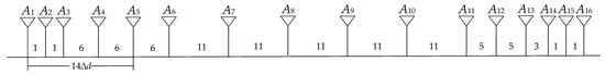
Figure 1.
Antenna array.

Table 1.
The system parameters.
Under normal circumstances, there are measurement errors or noise interference in actual measurements. Therefore, the corrupted visibility function samples are generated by applying additive Gaussian noise to the visibility function obtained by performing forward simulations on SAIR brightness temperature distributions according to Equation (3). Moreover, the regularization matrix of the Tikhonov regularization is set as the identity matrix, and multi-parameter regularization is represented by three-parameter regularization, in which the regularization matrices D1, D2, and D3 are taken as the identity matrix, first-order differential matrix, and second-order differential matrix, respectively.
In addition, total variation (TV) regularization is introduced as a comparison algorithm [27]. The TV regularization uses L1-norm instead of L2-norm regularization term of the Tikhonov regularization. In the paper, the TV regularization is solved by alternating direction method of multipliers (ADMM) algorithm in a previous study [28].
4.1. Experiment 1
In the first experiment, the performances of all the regularization approaches are evaluated by the use of the original distribution, which derives from the L-band brightness temperature data of the H polarization in the ocean area observed by the Aquarius satellite on 21, August, 2013. The original brightness temperature distribution is shown in Figure 2, where the horizontal axis ξ = sin θ is the direction cosines in the Cartesian coordinates and θ is the incidence angle in the across-track dimension measured from the nadir.
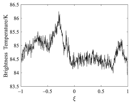
Figure 2.
The original brightness temperature distribution of the ocean.
When the measured visibility function samples are corrupted by white Gaussian noise with zero mean and variance σ2 = 0.01 max (Vi), the reconstructed results in the alias-free field of view are shown in Figure 3 via Tikhonov, band-limited and multi-parameter regularization. In Figure 3, the horizontal axes ξ = sin θ is the direction cosines in the Cartesian coordinates. For the convenience of comparison, the original distribution in the alias-free field of view is also shown in Figure 3. The results show that the retrieved distributions by the TV, Tikhonov, and band-limited regularization have obvious oscillation ripples, particularly at the edge of the distributions. This is because SAIRs can only cover the limited bandwidth in the frequency domain, which will result in the ripple oscillation, namely the Gibbs phenomenon. In general, the Gibbs effect can be reduced by applying windows such as the Blackman, Kaiser, and Hanning windows [29]. However, windowing needs to be at the cost of reducing the spatial resolution of the reconstructed map. Compared with the TV, Tikhonov and band-limited regularization, the retrieved distribution by the multi-parameter regularization is distinctly smoother and has weaker ripples especially on the edge of the distribution, which indicates that the multi-parameter regularization can retain more detailed information and better suppress the Gibbs effect.
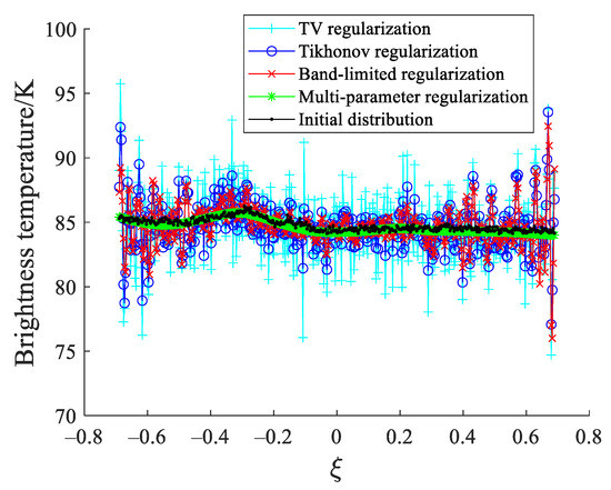
Figure 3.
Reconstructed results of the ocean in the alias-free field of view.
The reconstruction errors between the reconstructed results and the original distribution are quantitatively evaluated by the root mean square error (RMSE) and peak signal to noise ratio (PSNR). In Figure 3, the RMSE values for the TV, Tikhonov, band-limited regularization, and multi-parameter regularization are, respectively, 2.64 K, 1.71 K, 1.48 K, and 0.24 K, and the PSNR values for the TV, Tikhonov, band-limited, and multi-parameter regularization are, respectively, 39.70 dB, 43.46 dB, 44.74 dB, and 60.66 dB.
Moreover, the parameter of the Tikhonov regularization in Figure 3 is set as 0.62, and three parameters α1, α2, and α3 of multi-parameter regularization are 0.62, 5.22, and 420.86, respectively. The multi-parameter regularization is somewhat similar to the single-parameter Tikhonov regularization in form. As a consequence, we make a comparison between the multi-parameter regularization and the Tikhonov regularization with different parameters, and the performance comparison result is shown in Figure 4. In Figure 4, the horizontal axis is the logarithmic value log10(α/α0), where α is the parameter of the Tikhonov regularization and α0 = 0.62, is the regularization parameter selected by the GCV method. As can be seen from Figure 4, the regularization parameter has an important influence on the reconstruction performance of the Tikhonov regularization. Even if the Tikhonov regularization has an optimal parameter, its RMSE is still higher than that of the multi-parameter regularization.
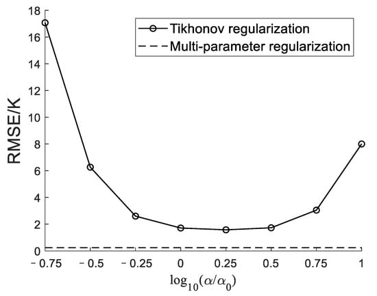
Figure 4.
The performance comparison between the multi-parameter regularization and the Tikhonov regularization with different parameters.
For the sake of analyzing quantitatively the influence of the noise on the reconstructed results, the corrupted visibility function samples with different level noises are used to reconstruct SAIR brightness temperature maps. The RMSE and PSNR performance with different noise levels is presented in Figure 5. As can be seen from Figure 5, whether the noise level is high or low, the RMSE for the multi-parameter regularization is dramatically lower than that for the TV, Tikhonov, and band-limited regularization. In addition, the multi-parameter regularization has the significant PSNR improvement of more than 9 dB over the TV, Tikhonov, and band-limited regularization. The result demonstrates that the multi-parameter regularization is more robust to the noise interference than the TV, Tikhonov, and band-limited regularization. In consequence, the multi-parameter regularization can reduce the reconstruction error more effectively, compared to traditional TV, Tikhonov, and band-limited regularizations.
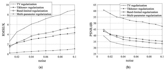
Figure 5.
The performance of the regularization methods for the ocean for different noise levels: (a) the root mean square error; (b) the peak signal to noise ratio.
4.2. Experiment 2
In the second experiment, the initial brightness temperature distribution, shown in Figure 6, is used to further evaluate the performances of all the reconstruction methods. The original distribution derives from the L-band brightness temperature data for the H polarization in the coast observed by the Aquarius satellite on 19 August 2013.
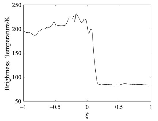
Figure 6.
The original brightness temperature distribution of the coastline.
The visibility function samples corrupted by Gaussian white noise with the variance σ2 = 0.01 max (Vi) are reconstructed using the TV, Tikhonov, band-limited, and multi-parameter regularization. The retrieved distributions in the alias-free field of view are presented in Figure 7. From Figure 7, we can find that the reconstruction results for the TV, Tikhonov, and band-limited regularization lost a lot of detailed information and have the obvious ripples on the edge of the map owing to the Gibbs effect. In addition, the multi-parameter regularization produces smoother and better results with clearer details particularly at the edge of the distribution, compared to the TV, Tikhonov, and band-limited regularizations. In order to quantitatively analyze the reconstruction errors, the RMSE and PSNR are calculated. In Figure 7, the RMSE values for the TV, Tikhonov, band-limited, total variation regularization, and multi-parameter regularization are 15.79 K, 4.91 K, 4.49 K, and 1.64 K, respectively, and the PSNR values for the TV, Tikhonov, band-limited, and multi-parameter regularization are 24.17 dB, 34.30 dB, 35.09 dB, and 43.84 dB, respectively.
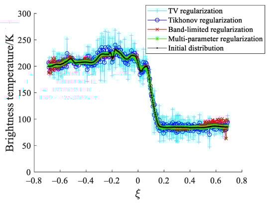
Figure 7.
Reconstructed results of the coast in the alias-free field of view.
Furthermore, the performance (RMSE and PSNR) of the TV, Tikhonov, band-limited, and multi-parameter regularization with different noise levels is shown in Figure 8 to quantitatively analyze the sensitivity of the above reconstruction methods to the error and noise interference. The results indicate that compared with the TV, Tikhonov, and band-limited regularization methods, the multi-parameter regularization is more robust to measurement error and noise interference. This seems to suggest that the multi-parameter regularization can better improve the accuracy of reconstructing the brightness temperature distributions.
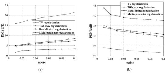
Figure 8.
The performance comparison of the regularization approaches for the coast for different noise levels: (a) the root mean square error; (b) the peak signal to noise ratio.
4.3. Experiment 3
For the sake of further verifying the robustness of the multi-parameter regularization, we have conducted the simulation experiment using two-dimensional brightness temperature image. The original image is shown in Figure 9a, where there are thirty brightness temperature bands of different ocean regions in the along-track direction. Because the result of a single measurement for the Aquarius satellite has only three brightness temperature bands, the original image comes from the results of ten measurements, which are randomly selected from the L-band brightness temperature data for the H polarization between 19, August and 21, August. When the variance of the additive Gaussian noise is set as σ2 = 0.01 max (Vi), the reconstructed image by different regularization methods in the alias-free field of view are presented in Figure 9b–e. Figure 9 indicates that there are obvious oscillation ripples for the inversion results of the TV, Tikhonov, and band-limited regularizations. Compared with the above three regularization methods, the oscillation ripples for the inversion result of multi-parameter regularization are effectively suppressed.
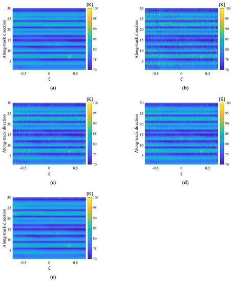
Figure 9.
Reconstructed image by different regularization methods in the alias-free field of view: (a) the original image; (b) TV regularization; (c) Tikhonov regularization; (d) band-limited regularization; (e) multi-parameter regularization.
The reconstruction error maps for different regularization methods are shown in Figure 10. From Figure 10, we could see that the reconstruction errors for the multi-parameter regularization are greatly diminished, compared with the TV, Tikhonov, and band-limited regularizations.
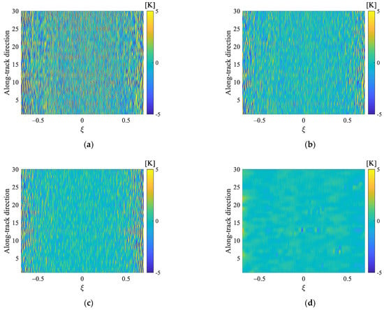
Figure 10.
Reconstruction error maps for different regularization methods: (a) TV regularization; (b) Tikhonov regularization; (c) band-limited regularization; (d) multi-parameter regularization.
To quantitatively analyze the reconstruction error in Figure 10, we calculated the performance (RMSE and PSNR) for each strip in the along-track direction. The relation between different strips and the performance of the regularization methods is presented in Figure 11. In Figure 11, the horizontal axis denotes the serial number of the strip, and the vertical axis is the RMSE and PSNR for the corresponding strip. Figure 11 indicates that when the strip changes, the performance of the TV regularization is obviously worse than other regularization methods, and the RMSE and PSNR for the band-limited regularization are close to those for the Tikhonov regularization. Moreover, even though the strips are different, the multi-parameter regularization has a considerably lower RMSE and a considerably higher PSNR than the TV, Tikhonov and band-limited regularizations. In consequence, the simulation experiment results show that the multi-parameter regularization is more robust to the measurement noise interference and the brightness temperature distributions of the observed scenes, which demonstrates the effectiveness of the proposed approach.
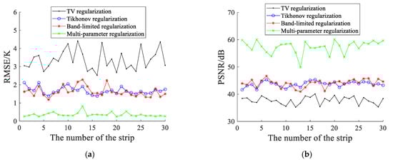
Figure 11.
The relation between different strips and the performance of the regularization methods: (a) the root mean square error; (b) the peak signal to noise ratio.
The computation time of the multi-parameter regularization method is closely related to the number of regularization parameters that need to be selected. When the size of G is 241 × 600, the MATLAB runtime (MATLAB2020a on a PC with 3.6 GHz Intel i9-9900 k processor and 64 GB memory) of the multi-parameter regularization with three parameters are 0.0924 s. Moreover, the MATLAB runtime of the TV, Tikhonov, and band-limited regularizations are 0.0114 s, 0.0312 s, and 0.0129 s, respectively. The results indicate that the calculation time of the three-parameter regularization is about three times that of the Tikhonov regularization. In consequence, the multi-parameter regularization increases the computational and memory cost while improving the accuracy of the reconstructed brightness temperature maps. The factorization technique or the approximate solution of Equation (8) may be introduced to reduce the computational complexity. Moreover, the program can run on the graphics processing unit (GPU) platform to increase the speed of computation.
5. Conclusions
The reconstruction of the brightness temperature map of the observed scene in SAIRs has been demonstrated to be an ill-posed inverse problem, which needs to be regularized to provide a unique and stable solution. Although the conventional regularization approaches such as the TV, Tikhonov, and band-limited regularizations can effectively alleviate the ill-conditioned features of the inverse problem, it may not preserve multi-scale features of the original maps because of only adding a single constraint. Different from some inverse problems, where there may be a clear best choice of regularization restriction and parameter, the inverse problem of SAIRs is complicated so that choosing any particular restriction brings advantages and disadvantages, even when a suitable regularization parameter is selected.
In response to the above issue, we propose a multi-parameter regularization method with multiple constraints for SAIR reconstruction in this paper. Instead of using a single penalty, multi-parameter regularization adds multiple different penalties to reflect multi-scale characteristics of the original map. Furthermore, regularization parameters are chosen by utilizing the simplified multi-dimensional generalized cross-validation method. Several simulation experiments were carried out on the FPIR system. The results reveal that the multi-parameter regularization can retain more detailed information and better suppress the Gibbs effect than the TV, Tikhonov, and band-limited regularizations, indicating probably the effectiveness of the proposed method. Moreover, the multi-parameter regularization approach can better suppress noise and exhibit the significant improvement of the reconstruction performance like RMSE and PSNR, compared to the traditional regularization methods.
Author Contributions
Data curation, J.Y. and L.W.; Funding acquisition, X.Y. and M.J.; Methodology, X.Y. and Z.Y.; Supervision, J.Y., L.W. and M.J.; Validation, X.Y. and Z.Y.; Writing—original draft, X.Y. and Z.Y.; Writing—review & editing, X.Y. and Z.Y. All authors have read and agreed to the published version of the manuscript.
Funding
This research was funded in part by the Zhejiang Provincial Natural Science Foundation of China under Grant LY18D060009, in part by the National Natural Science Foundation of China under Grant 61672466, in part by the Joint Fund of Zhejiang Provincial Natural Science Foundation under Grant LSZ19F010001, in part by the Key Research and Development Program of Zhejiang Province under Grant 2020C03060.
Institutional Review Board Statement
Not applicable.
Informed Consent Statement
Not applicable.
Data Availability Statement
Data sharing not applicable.
Conflicts of Interest
The authors declare no confict or interest.
References
- Martin-Neira, M.; LeVine, D.M.; Kerr, Y. Microwave Imaging radiometry in remote sensing: An invited historical review. Radio Sci. 2014, 49, 415–449. [Google Scholar] [CrossRef]
- Reising, S.C.; Gaier, T.C.; Kummerow, C.D.; Padmanabhan, S.; Berg, W. Temporal Experiment for Storms and Tropical Systems Technology Demonstration (TEMPEST-D): Reducing risk for 6U-Class nanosatellite constellations. In Proceedings of the 2016 IEEE International Geoscience and Remote Sensing Symposium (IGARSS), Beijing, China, 10–15 July 2016. [Google Scholar]
- Kpré, E.; Vellas, N.; Gaquiére, C.; Decroze, C.; Fromentèze, T.; Mouhamadou, M. A Compressive Millimeter-Wave Imaging Imager for Security Applications. In Proceedings of the 2018 IEEE International Symposium on Antennas and Propagation & USNC/URSI National Radio Science Meeting, Boston, MA, USA, 8–13 July 2018. [Google Scholar]
- Levine, D.M.; Griffis, A.J.; Swift, C.T.; Jackson, T.J. ESTAR: A synthetic aperture microwave radiometer for remote sensing spplications. Proc. IEEE 1994, 82, 1787–1801. [Google Scholar] [CrossRef]
- Corbella, I.; Torres, F.; Duffo, N.; Gonzalez-Gambau, V.; Pablos, M.; Duran, I.; Martin-Neira, M. MIRAS calibration and performance: Results from the SMOS in-orbit commissioning phase. IEEE Trans. Geosci. Remote Sens. 2011, 49, 3147–3155. [Google Scholar] [CrossRef]
- Tanner, A.B.; Wilson, W.J.; Lambrigsten, B.H.; Dinardo, S.J.; Brown, S.T.; Kangaslahti, P.P.; Gaier, T.C.; Ruf, C.S.; Gross, S.M.; Lim, L.B.H.; et al. Initial Results of the Geostationary Synthetic Thinned Array Radiometer (GeoSTAR) Demonstrator Instrument. IEEE Trans. Geosci. Remote Sens. 2007, 45, 1947–1957. [Google Scholar] [CrossRef]
- Zhang, C.; Liu, H.; Wu, J.; Zhang, S.; Yan, J.; Niu, L.; Sun, W.; Li, H. Imaging analysis and first results of the geostationary interferometric microwave sounder demonstrator. IEEE Trans. Geosci. Remote Sens. 2015, 53, 207–218. [Google Scholar] [CrossRef]
- Anterrieu, E. A resolving matrix approach for synthetic aperture imaging radiometers. IEEE Trans. Geosci. Remote Sens. 2004, 42, 1649–1656. [Google Scholar] [CrossRef]
- Picard, B.; Anterrieu, E. Comparison of regularized inversion methods in synthetic aperture imaging radiometry. IEEE Trans. Geosci. Remote Sens. 2005, 43, 218–224. [Google Scholar] [CrossRef]
- Liang, W.; Fei, H.; Feng, H.; Li, J. Bayesian Inference for Inversion in Synthetic Aperture Imaging Radiometry. IEEE Geosci. Remote Sens. 2016, 13, 1049–1053. [Google Scholar]
- Zhang, Y.; Ren, Y.; Miao, W.; Lin, Z.; Gao, H.; Shi, S. Microwave SAIR Imaging Approach Based on Deep Convolutional Neural Network. IEEE Trans. Geosci. Remote Sens. 2019, 57, 10376–10389. [Google Scholar] [CrossRef]
- Yang, X.; Yang, Z.; Yan, J.; Wu, L.; Lyu, W. Reduction of the Reconstruction Error With Lower and Upper Bounds in Synthetic Aperture Imaging Radiometers. IEEE Access 2020, 8, 156964–156971. [Google Scholar] [CrossRef]
- Martin-Neira, M.; Oliva, R.; Corbella, I.; Torres, F.; Duffo, N.; Duran, I.; Kainulainen, J.; Closa, J.; Zurita, A.; Cabot, F.; et al. SMOS instrument performance and calibration after six years in orbit. Remote Sens. Environ. 2016, 180, 19–39. [Google Scholar] [CrossRef]
- Belge, M. Multiscale and Curvature Methods for the Regularization of the Linear Inverse Problems; Northeastern University: Boston, MA, USA, 1999. [Google Scholar]
- Brezinski, C.; Redivo-Zaglia, M.; Rodriguez, G.; Seatzu, S. Multi-parameter regularization techniques for ill-conditioned linear systems. Numer. Math. 2003, 94, 203–228. [Google Scholar] [CrossRef]
- Chen, Z.; Yao, L.; Xu, Y.; Ynag, H. Multi-parameter tikhonov regularization for linear ill-posed operator equations. J. Comput. Math. 2008, 26, 37–55. [Google Scholar]
- Wang, Z. Multi-parameter Tikhonov regularization and model function approach to the damped Morozov principle for choosing regularization parameters. J. Comput. Appl. Math. 2012, 236, 1815–1832. [Google Scholar] [CrossRef]
- Brooks, D.H.; Ahmad, G.F.; MacLeod, R.S.; Maratos, G.M. Inverse electrocardiography by simultaneous imposition of multiple constraints. IEEE Trans. Biomed. Eng. 1999, 46, 3–18. [Google Scholar] [CrossRef] [PubMed]
- Jiang, D. A Multi-parameter Regularization Model for Deblurring Images Corrupted by Impulsive Noise. Circ. Syst. Signal Pr. 2017, 36, 3702–3730. [Google Scholar] [CrossRef]
- Zhang, W.; Shen, J.; Thomas, J.C.; Mu, T.; Zhu, X. Particle size distribution recovery in dynamic light scattering by optimized multi-parameter regularization based on the singular value distribution. Powder Technol. 2019, 353, 320–329. [Google Scholar] [CrossRef]
- Aucejo, M.; De Smet, O. Multi-parameter multiplicative regularization: An application to force reconstruction problemse. J. Sound Vib. 2020, 469, 115–135. [Google Scholar] [CrossRef]
- Corbella, I.; Duffo, N.; Vall-llossera, M.; Camps, A.; Torres, F. The visibility function in Imaging aperture synthesis radiometry. IEEE Trans. Geosci. Remote Sens. 2004, 42, 1677–1682. [Google Scholar] [CrossRef]
- Hansen, P.C.; O’Leary, D.P. The use of the L-curve in the regularization of discrete ill-posed problems. SIAM J. Sci. Comput. 1993, 14, 1487–1503. [Google Scholar] [CrossRef]
- Craven, P.; Wahba, G. Smoothing noisy data with spline functions: Estimating the correct degree of smoothing by the method of Generalized Cross Validation. Numer. Math. 1979, 31, 377–403. [Google Scholar] [CrossRef]
- Wahba, G. Spline Models for Observational Data; Society for Industrial and Applied Mathematics: Philadelphia, PA, USA, 1990; pp. 1–169. [Google Scholar]
- Wu, L.; Yan, J.; Zhao, F.; Lan, A.; Wu, J. FPIR: Demonstrator Integration and Ground-Based Salinity Observation Experiment. In Proceedings of the IGARSS 2018—2018 IEEE International Geoscience and Remote Sensing Symposium, Valencia, Spain, 22–27 July 2018. [Google Scholar]
- Rudin, L.I.; Osher, S.; Fatemi, E. Nonlinear total variation based noise removal algorithms. Phys. D Nonlinear Phenom. 1992, 60, 259–268. [Google Scholar] [CrossRef]
- Boyd, S.; Parikh, N.; Chu, E.; Peleato, B.; Eckstein, J. Distributed Optimization and Statistical Learning via the Alternating Direction Method of Multipliers. Found. Trends Mach. Learn. 2010, 3, 1–122. [Google Scholar] [CrossRef]
- Anterrieu, E.; Waldteufel, P.; Lannes, A. Apodization functions for 2-D hexagonally sampled synthetic aperture imaging radiometers. IEEE Trans. Geosci. Remote Sens. 2002, 40, 2531–2542. [Google Scholar] [CrossRef]


Publisher’s Note: MDPI stays neutral with regard to jurisdictional claims in published maps and institutional affiliations. |
© 2021 by the authors. Licensee MDPI, Basel, Switzerland. This article is an open access article distributed under the terms and conditions of the Creative Commons Attribution (CC BY) license (http://creativecommons.org/licenses/by/4.0/).