Estimating Leaf Nitrogen Content in Corn Based on Information Fusion of Multiple-Sensor Imagery from UAV

Abstract

With the rapid development of unmanned aerial vehicle (UAV) and sensor technology, UAVs that can simultaneously carry different sensors have been increasingly used to monitor nitrogen status in crops due to their flexibility and adaptability. This study aimed to explore how to use the image information combined from two different sensors mounted on an UAV to evaluate leaf nitrogen content (LNC) in corn. Field experiments with corn were conducted using different nitrogen rates and cultivars at the National Precision Agriculture Research and Demonstration Base in China in 2017. Digital RGB and multispectral images were obtained synchronously by UAV in the V12, R1, and R3 growth stages of corn, respectively. A novel family of modified vegetation indices, named coverage adjusted spectral indices (CASIs (CASI $=\mathrm{VI}/\left(1+{\mathrm{FV}}_{\mathrm{cover}}\right)$, where VI denotes the reference vegetation index and ${\mathrm{FV}}_{\mathrm{cover}}$ refers to the fraction of vegetation coverage), has been introduced to estimate LNC in corn. Thereby, typical VIs were extracted from multispectral images, which have the advantage of relatively higher spectral resolution, and ${\mathrm{FV}}_{\mathrm{cover}}$ was calculated by RGB images that feature higher spatial resolution. Then, the PLS (partial least squares) method was employed to investigate the relationships between LNC and the optimal set of CASIs or VIs selected by the RFA (random frog algorithm) in different corn growth stages. The analysis results indicated that whether removing soil noise or not, CASIs guaranteed a better estimation of LNC than VIs for all of the three growth stages of corn, and the usage of CASIs in the R1 stage yielded the best R² value of 0.59, with a RMSE (root mean square error) of 22.02% and NRMSE (normalized root mean square error) of 8.37%. It was concluded that CASIs, based on the fusion of information acquired synchronously from both lower resolution multispectral and higher resolution RGB images, have a good potential for crop nitrogen monitoring by UAV. Furthermore, they could also serve as a useful way for assessing other physical and chemical parameters in further applications for crops.

1. Introduction

Nitrogen is a critical nutrient element for crop growth. The proper application of nitrogen fertilizer has a significant influence on final crop yield and quality. Leaf nitrogen in crop canopies is an important indicator that characterizes the nitrogen nutrition status in crops. Accurate and dynamic estimation of crop leaf nitrogen is of significance for rationally managing nitrogen fertilization [1,2].

Conventional methods for detecting crop nitrogen usually involve outdoor sampling and indoor testing, which is not only time-consuming and laborious but also destructive and lagging. With the development of spectral detection technology, non-destructive remote sensing has become an attractive tool for crop nitrogen assessment. For regional-scale monitoring of crop nitrogen, satellite-based optical remote-sensing technology is widely used, but at a field scale it is often hindered by cloud cover and high cost [3]. In recent years, family farms have gradually become an important mode of operation in Chinese agriculture, and there is a great demand for new technologies. As a rapidly developing technology, with the advantages of high efficiency, low cost, and convenience of use [4,5,6], UAVs (unmanned aerial vehicle) have begun to play an active role in agricultural field management [7,8,9]. The spatial resolution of UAV images can reach centimeter or even millimeter scales, which has unparalleled advantages on the field scale for diagnosing crop nitrogen nutrition in family farms. Recently, there have been many reports on crop nitrogen assessment using UAVs. Some vegetation indices (VI) and spectral bands from UAV-based multispectral imagery have been used with machine learning methods to effectively predict leaf nitrogen content (LNC) in maize [10], and have also been employed to evaluate the nitrogen accumulation in corn canopies, and map the spatial nitrogen variation in corn fields [11]. UAV-based hyperspectral data with plenty of shallow bands had a good performance for evaluating LNC in the different growth stages of wheat [12]. The combined features of vegetation coverage and VIs extracted from UAV-based RGB images could show some potential for estimating LNC in maize [13]. In addition, UAV-based images from RGB, multispectral, and thermal sensors have been used to acquire vegetation and temperature parameters for assessing nitrogen use efficiency in crops [14].

It is noted that UAV images have a higher spatial resolution compared with conventional satellite images, and the problem of soil background affecting crop canopy spectra is more prominent. Knowing how to decrease the influence of soil noise as much as possible is vital to the accurate estimation of crop nitrogen by remote sensing [15]. A few vegetation indices (VIs) have been developed to eliminate or minimize the effects of soil background. Huete et al. [15] proposed the soil adjusted vegetation index (SAVI) to describe soil–vegetation systems, and lessen the sensitivity of vegetation indices (VIs) to soil background. Rondeaux et al. [16] recommended the optimized SAVI (OSAVI) to increase the response to vegetation, while decreasing the variability from the soil. Due to changes of soil humidity and solar incidence angle, Major et al. [17] suggested three modified SAVIs (SAVI2, SAVI3, and SAVI4) to alleviate the influence of soil background. In the above studies, these VIs were designed to generally decrease soil noise by adding an adjusting factor into the combination of both red and near-infrared reflectance bands, usually suitable for remote sensing images with relatively low spatial resolution or more mixed pixels. Liu et al. [18] used three threshold methods with RGB digital images from UAV to separate wheat from soil, and then evaluate nitrogen status in wheat with RGB-based VIs. Yao et al. [19] developed a coverage adjustment spectral index (CASI), into which fractional vegetation cover (${\mathrm{FV}}_{\mathrm{cover}}$) was introduced to monitor LNC in winter wheat with ground hyperspectral measurements under different soil backgrounds, and obtained a better accuracy of LNC estimation. In the existing reports on crop nitrogen assessment, the selected VIs are usually calculated only using the UAV images from a single sensor, even if there are multi-sensor images acquired synchronously from an aerial platform, and it is seldom considered that, in terms of the complementary advantages of different sensors in spatial and spectral resolution, the multiple-sensor images could be simultaneously applied to extract some VIs for crop nitrogen evaluation. Possibly, VIs using a fusion of information will have a better performance in assessing nitrogen status in crops.

The above mentioned CASI (CASI $=\mathrm{VI}/\left(1+{\mathrm{FV}}_{\mathrm{cover}}\right)$) could decrease the influence of soil noise, and has been proved to be effective in estimating LNC in wheat, but both the VI and ${\mathrm{FV}}_{\mathrm{cover}}$ in CASI were calculated by ground canopy spectral measurements and digital pictures, respectively, not using UAV remote sensing images [19]. Hence, it is worth discussing whether CASI is also adaptable to estimate LNC in corn when using UAV-based multi-sensor images, and at present little research on this has been conducted. In this study, CASI was tested to evaluate LNC in corn using UAV multi-sensor images. Digital RGB and multispectral images were acquired synchronously from UAV sensors at three growth stages of corn. Considering that multispectral images have the advantage of relatively higher spectral resolution, and RGB images are characterized by higher spatial resolution, the two inputs, VI and ${\mathrm{FV}}_{\mathrm{cover}}$, into CASI were extracted from multispectral and RGB images, respectively. Thereby, CASI could make use of the complementary advantages of different sensors in spatial and spectral resolution, and integrated the useful information from two sensors. This might be helpful to effectively assess nitrogen status in crops.

This study focuses on the potential applications of both UAV multi-sensor images and the modified vegetation index, CASI, for LNC assessment. The objectives of this study were: (i) to evaluate the potential performance of CASI for LNC estimates using UAV-based data; (ii) to compare the ability of the selected existing VI and the corresponding CASI to reduce the influence of soil noise; (iii) to provide a new concept and method reference using UAV multi-sensor images to monitor nitrogen status in crops.

2. Materials and Methods

2.1. UAV System

In this present study, an eight-rotor electric UAV carrying digital RGB and multispectral cameras was used to collect images in the study area. A DJI-S1000+ (DJI, Guangdong, China) was chosen as the UAV flight platform, which weighs 4.4 kg, and has an automated flight control system allowing for user-defined waypoint operations and custom mission planning, a maximum flight time of 20 min, and a LiPo battery (6S, 10,000~20,000 mAh). The digital RGB imager carried by the UAV was equipped with a high-definition Cyber-shot DSC-QX100 camera (Sony, Minato, Tokyo, Japan) that weighs 179 g and uses an Exmor R CMOS sensor with an effective 20 megapixels. A Parrot Sequoia (Parrot, USA) multispectral camera which consists of four single-band photoreceptors with 1.2 megapixels was also mounted on the UAV; the Sequoia camera weighs 107 g and has built-in 64 GB storage and SD expansion slots. More details about the parameters of the sensors are in

Table 1. Main parameters of the sensors mounted on the UAV in this study.

Sensor Name	Sensor Type	Spectral Band (nm)	Resolution (pixels)	FOV (H° × V°)	Shutter Type	Weight (g)
Parrot Sequoia	MS	550, 660, 735, 790 *	1280 × 960	62.2 × 48.7	Global	107
Cyber-shot DSC-QX100	RGB	N/A	5472×3648	82.0 × 64.5	Global	179

MS: multispectral, FOV: field of view, H: horizonal, V: vertical. * for convenience, the 550 nm band is denoted by GRE, 660 nm RED, 735 nm REG, and 790 nm NIR in the subsequent analyses.

.

2.2. Data Collection and Acquisition

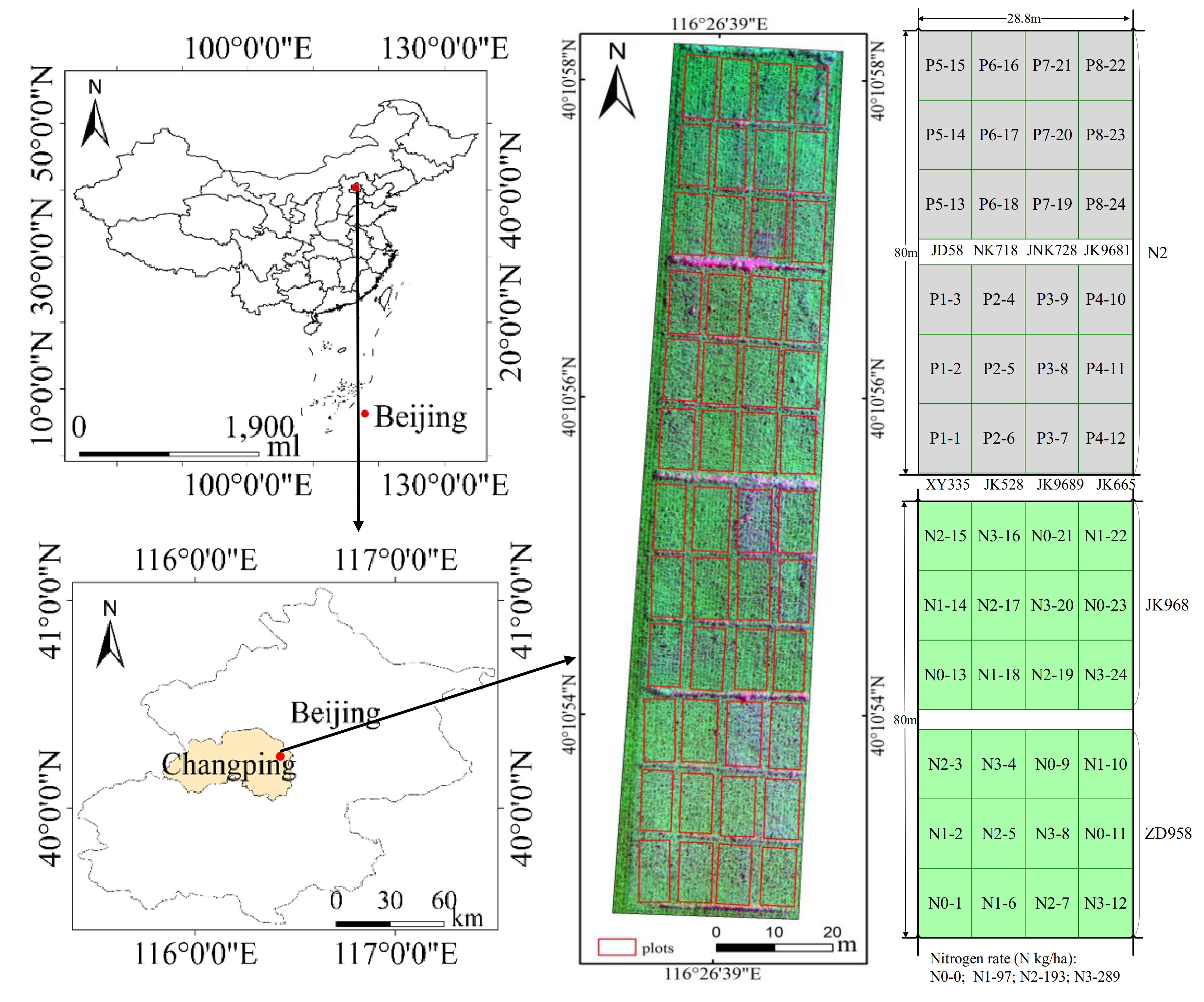
2.2.1. Study Site and Experimental Design

The experiment was conducted at the National Precision Agriculture Research Demonstration Base in 2017. The base is located in the northeast of Xiaotangshan Town, Changping District, Beijing (40°00′–40°21′N, 116°34′–117°00′E, 36 m). There is a temperate continental monsoon climate in this area, and the soil is a moist and heavy loam, with a nitrate N (NO₃-N) content of 3.2–14.8 mg/kg, an ammonium nitrogen (NH₄-N) content of 10.2–12.3 mg∙kg⁻¹, an available phosphorus content of 3.1–21.2 mg∙kg⁻¹, an effective potassium content of 86.8–120.6 mg∙kg⁻¹, and an organic matter content of 15.8–20.2 g∙kg⁻¹.

The experiment involved 48 plots, among which 24 plots concerned different cultivars (P) in the north and the other 24 were linked with nitrogen (N) rates in the south, each plot was 6 × 10 m, with a 1 m isolation zone (Figure 1). Eight cultivars were selected for sowing, with three repetitions for each cultivar in the northern experiment field, and among the eight cultivars: four (JK9681, JK528, JK9689, and JK665) belong to the JingKe (JK) corn family in China; two (NK718 and JNK728) are widely cultivated in Northeast China and the northern regions of North China, and have some differences in disease resistance and maturity; and another two (JD58 and XY335) are high-yielding and early-maturing varieties in North China. For 24 plots in the north of the experiment field, N fertilizer treatment was the conventional N rate (N2): 193 kg∙ha⁻¹. In the southern half of experiment field, the 24 plots were treated with the following N rates: no nitrogen application (N0), 97 kg∙ha⁻¹ (N1), 193 kg∙ha⁻¹ (N2), and 289 kg∙ha⁻¹ (N3), each N treatment was repeated six times, and the two cultivars (JK968 and ZD958) that are the most widely cultivated in North China were selected to sow in the 12 plots (Figure 1). Management procedures, such as pest management, weed control, and phosphate and potassium application in all plots were carried out according to local practical standards.

2.2.2. Determination of Leaf Nitrogen Concentration

This experiment covered the three important growth stages, the V12, R1, and R3 stages of summer corn. V12 is a critical stage during corn vegetative growth, the twelfth leaf of the corn plant is fully unfolded, and the female ear begins floret differentiation in the V12 stage. R1 belongs to the transition period from vegetative growth to reproductive growth, and in this stage the filament of the female ear emerges from the bract. R3 is an important stage during corn reproductive growth, and the corn seeds turn yellow in the R3 stage [20]. In the three stages, the differences of corn canopy structure are relatively obvious and representative, which can result in different influences of the soil background on canopy spectra.

The collections of ground samples were conducted on 7 and 18 August, and 1 September in 2017. Three representative corn plants were selected in each of the forty-eight plots, and the aboveground corn plants were collected for subsequent analysis. In laboratory conditions, the green leaves of the three corn plants from each plot were separated from stems and de-enzymed at 105 °C for 30 min, and then dried at 80 °C to constant weight for chemical analysis. LNCs (g 100 g⁻¹, %) for the dried leaf samples were determined by a Kjeldahl meter (Buchi B–339, FOSS, Sweden).

Table 2. Descriptive statistics for measured corn leaf nitrogen content (LNC) from three growth stages.

Growth Stage	Sample Number	Max	Min	Mean	SD	CV
V12	48	3.17	1.42	2.38	0.43	0.18
R1	48	3.49	1.17	2.63	0.35	0.13
R3	48	3.36	1.37	2.36	0.45	0.19

SD: standard deviation, CV: coefficient of variation.

shows the statistics for the measured LNC.

2.3. Methods and Principles

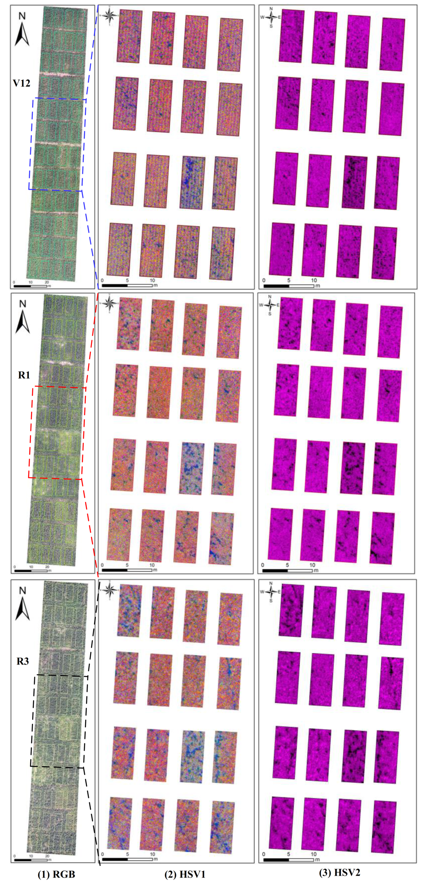
2.3.1. Image Acquisition

UAV surveys with two camera sensors collecting digital RGB and multispectral imagery were conducted under clear and cloudless weather conditions from 10:00 a.m. to 14:00 p.m. on 7 and 18 August, and 1 September in 2017. The UAV missions investigating the 48 plots were performed at a flight height of 60 m and a flight speed of 6 m∙s⁻¹, with a tilt angle of 0° for the two cameras, and a shortest interval of 2 s between imagery acquisitions. Both the front overlap and the side overlap of UAV flights were set to 80%.

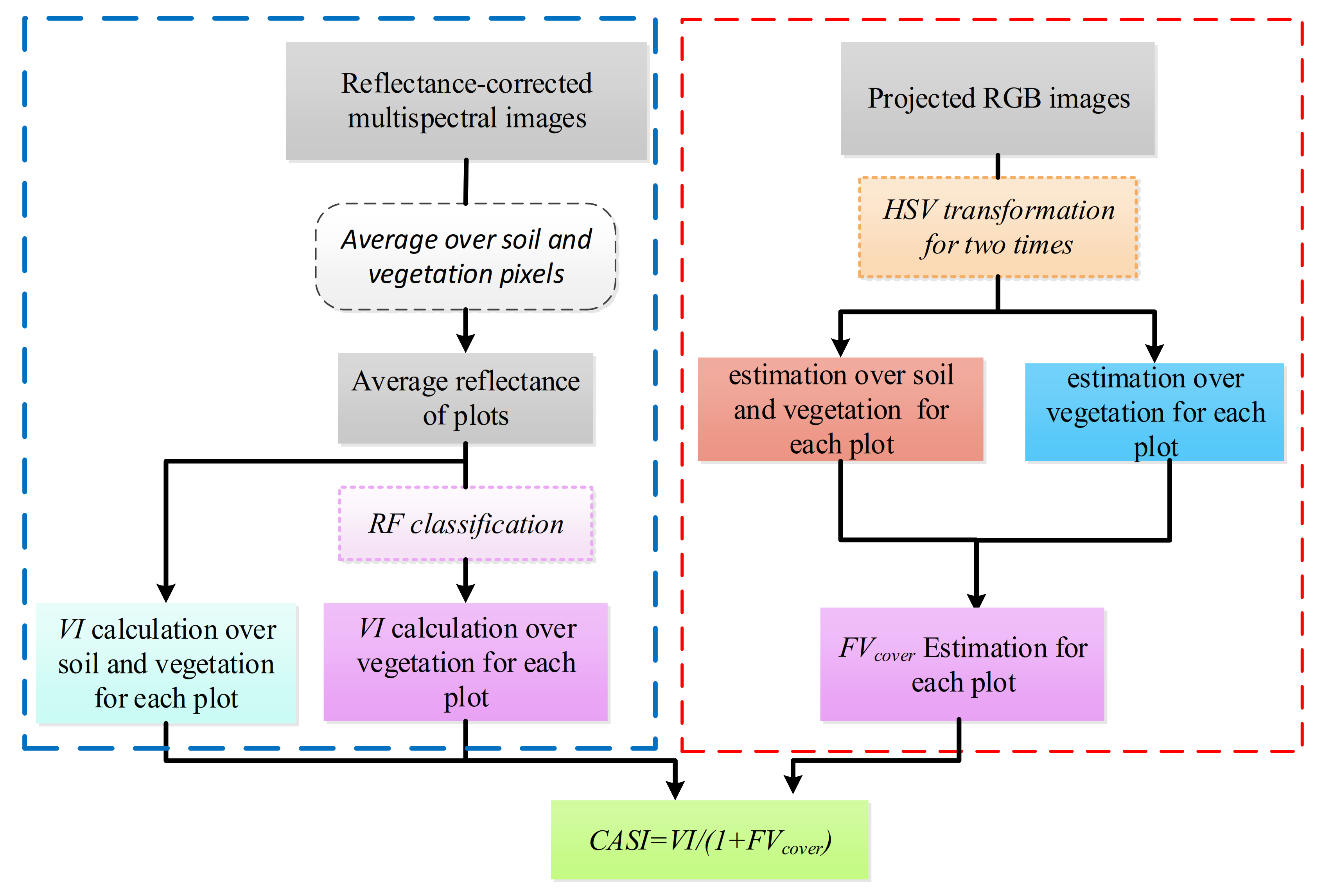
2.3.2. Image Processing

It has been proven that high-definition digital images can be transformed into new color spaces by HSV (hue saturation value), and it is very easy to distinguish soil from vegetation in the HSV-based images [21,22]. In this study, the colors (red, green, blue) of digital RGB images from the UAV were converted into hue, saturation, and value by HSV, and then threshold segmentation was used to differentiate between vegetation and soil in the images. Figure 2 shows the spatial color transformation distribution of the study area. It can be seen that after the original RGB images have been transformed by HSV two times, the soil is able to be clearly distinguished from crop vegetation in the HSV2 images.

Some existing studies have demonstrated that random forest classification (RFC) can be well adopted for medical disease classification, habitat identification in ecological environments, and land cover classification based on multispectral images [23,24,25]. For the UAV multispectral images in this study, RFC was implemented to differentiate between vegetation and soil, and then created a vector including corn vegetation and soil.

2.3.3. Vegetation Coverage

Fractional vegetation coverage (${\mathrm{FV}}_{\mathrm{cover}}$), which refers to the percentage of vertical projection area of vegetation per ground surface area, is a critical parameter for assessing crop density and soil factor. Ground-based RGB images have been used to effectively extract vegetation coverage by methods of color transformation and threshold segmentation [26,27]. By comparison, UAV-based RGB images have the distinct advantages of monitoring a large-scale area, as well as high spatial resolution, which facilitate the acquisition of vegetation coverage and the evaluation of crop growth in fields. In the present study, RGB images derived from UAV were converted into new image data via two HSV transformations, so as to identify background soil and corn canopy area more easily [21]. Identified corn pixels in each plot were then divided by the total number of pixels in the same plot to acquire ${\mathrm{FV}}_{\mathrm{cover}}$. Vegetation coverage is calculated as follows:

$${\mathrm{FV}}_{\mathrm{cover}}=\frac{{\mathrm{A}}_{\mathrm{veg}}}{{\mathrm{A}}_{\mathrm{total}}}$$

(1)

where ${\mathrm{FV}}_{\mathrm{cover}}$ is the coverage of vegetation, ${\mathrm{A}}_{\mathrm{veg}}$ is the number of corn pixels in each plot, and ${\mathrm{A}}_{\mathrm{total}}$ is the total number of pixels in the same plot.

Yao et al. [19] proposed the novel index, CASI, to quantitatively correct for the effect of changing vegetation density and soil cover on wheat LNC estimates, on the basis of understanding the L parameters of SAVI previous studied. Namely, ${\mathrm{FV}}_{\mathrm{cover}}$ factor was added to VIs as follows: $\mathrm{CASI}=\mathrm{VI}/\left(1+{\mathrm{FV}}_{\mathrm{cover}}\right).$ However, the two inputs of CASI in the study of Yao et al., VI and ${\mathrm{FV}}_{\mathrm{cover}}$, were calculated by ground-based canopy spectra and digital RGB pictures in wheat fields, respectively. In the present study, the extraction of CASI was performed by using UAV-based images in the following framework (Figure 3).

2.3.4. Spectral Variables

Reflectance bands (green, red, red-edge, and near-infrared) from multispectral images derived from UAV were used as canopy spectral features, which were variably linked with plant activity, canopy structure, and nutrient situation [28,29,30]. Vegetation indices that can indicate crop nutrition and growth status have been widely used in agricultural fields. In this study, multispectral images were utilized to extract a set of VIs and the corresponding CASIs for LNC estimation.

Table 3. Vegetation indices from UAV-based multispectral images in the study.

VIs	Name	Formula	Reference
DVI	Difference Vegetation Index	$\mathrm{DVI}=R_{NIR}-R_{RED}$	[31]
GNDVI	Green NDVI	$\mathrm{GNDVI}=\left(R_{NIR}-R_{GRE}\right)/\left(R_{NIR}+R_{GRE}\right)$	[32]
MNLI	Modified Non-linear Vegetation Index	$\mathrm{MNLI}=1.5\left(R_{NIR}{}^2-R_{RED}\right)/\left(R_{NIR}{}^2+R_{RED}+0.5\right)$	[33]
MSAVI	Modified SAVI	$\mathrm{MSAVI}=\left(2R_{NIR}+1-\sqrt{{\left(2R_{NIR}+1\right)}^2-8\left(R_{NIR}-R_{RED}\right)}\right)/2$	[34]
MSR	Modified Simple Ratio	$\mathrm{MSR}=\left(R_{NIR}/R_{NIR}-1\right)/\sqrt{R_{NIR}/R_{NIR}+1}$	[35]
MTVI2	Modified Triangular Vegetation Index 2	$\mathrm{MTVI}2=\frac{1.5\left(1.2\left(R_{NIR}-R_{GRE}\right)-2.5\left(R_{RED}-R_{GRE}\right)\right)}{\sqrt{{\left(2R_{NIR}+1\right)}^2-\left(6R_{NIR}-5\sqrt{R_{RED}}\right)-0.5}}$	[36]
NDVI	Normalized Difference Vegetation Index	$\mathrm{NDVI}=\left(R_{NIR}-R_{RED}\right)/\left(R_{NIR}+R_{RED}\right)$	[37]
NLI	Non-linear Vegetation Index	$\mathrm{NLI}=\left(R_{NIR}{}^2-R_{RED}\right)/\left(R_{NIR}{}^2+R_{RED}\right)$	[38]
OSAVI	Optimization of Soil-Adjusted Vegetation Index	$\mathrm{OSAVI}=1.16\left(R_{NIR}-R_{RED}\right)/\left(R_{NIR}+R_{RED}+0.16\right)$	[16]
R_M	Red Model	$\mathrm{R}\_\mathrm{M}=R_{NIR}/R_{\mathrm{REG}}-1$	[39]
RDVI	Renormalized Difference Vegetation Index	$\mathrm{RDVI}=\left(R_{NIR}-R_{RED}\right)/\sqrt{R_{NIR}+R_{RED}}$	[40]
RVI	Ratio Vegetation Index	$\mathrm{RVI}=R_{NIR}/R_{RED}$	[41]
RVIgreen	Green Ratio Vegetation Index	${\mathrm{RVI}}_{\mathrm{green}}=R_{NIR}/R_{GRE}$	[42]
TVI	Triangular Vegetation Index	$\mathrm{TVI}=0.5\left(120\left(R_{NIR}-R_{GRE}\right)-200\left(R_{RED}-R_{GRE}\right)\right)$	[43]

Note: $R_{GRE}$ denotes green band reflectance, $R_{RED}$ red band reflectance, $R_{REG}$ red-edge band reflectance, and $R_{NIR}$ near-infrared reflectance.

lists the selected VIs that are related to the nitrogen status in crops.

2.3.5. Random Frog Algorithm

The random frog algorithm (RFA) is an effective tool for variable selection on the basis of the reversible jump Markov chain Monte Carlo method [44]. Generally, the RFA works in three steps: (1) randomly give an initial subset V₀ with Q variables; (2) propose a candidate subset V* containing Q* variables based on V₀, take V* with a certain probability as V₁, and then replace V₀ with V₁. Loop this step until N iterations; (3) calculate a selection probability of each variable, which will be used as a measure of variable importance and a criterion of variable selection [44,45,46]. In the present study, RFA was used to select the better variables among both four bands and a set of VIs or CASIs from UAV-based images for LNC estimation. First, all spectral variables were ranked in descending order, according to the selection probabilities computed by RFA, and then the top five variables were selected as the optimal features for evaluating N status in corn.

2.3.6. Partial Least Squares Regression

Partial least squares regression (PLSR) is a widely used technique for studying the relationships between multiple dependent variables and multiple independent variables. PLSR integrates the merits of principal component analysis (PCA), canonical analysis (CCA), and linear regression analysis, and can efficiently obtain the dominant factors with the strongest explanatory power for dependent variables. Especially, it is very useful for solving problems such as with obvious multicollinearity between variables, or when the number of variables is greater than the number of samples [47].

2.3.7. Data Evaluation

In this study VIs were extracted from UAV-based multispectral images before and after removing soil noise, and their correlations with LNC were analyzed, as well as the corresponding CASIs. The coefficient of determination (R²), root mean square error (RMSE), and normalized RMSE (NRMSE, %) were used to explain and quantify the relationship with LNC, and the three metrics can be expressed as follows:

$$R^2=1-{\Sigma }_{i=1}^n{(x_i-y_i)}^2/{\Sigma }_{i=1}^n{(x_i-\overline{x})}^2$$

(2)

$$\mathrm{RMSE}=\sqrt{{\Sigma }_{i=1}^n{(x_i-y_i)}^2/n}$$

(3)

$$\mathrm{NRMSE}=\frac{\mathrm{RMSE}}{\overline{x}}\ast 100$$

(4)

where $x_i$ and $y_i$ are the measured and predicted LNC in corn, $\overline{x}$ is the mean of measured LNC, and $n$ is the total number of samples.

3. Results

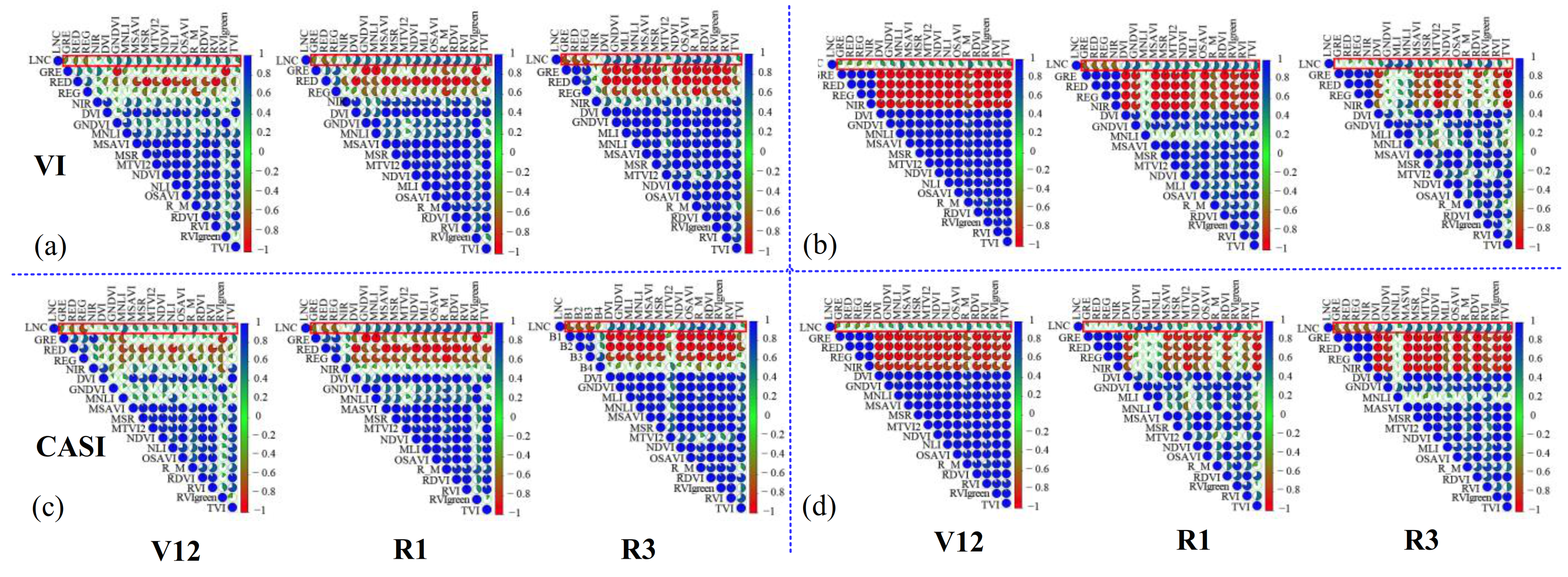
3.1. Relationship between VIs, CASIs, and LNC

Table 4. Correlations between LNC, VIs, and CASIs in the three growth stages.

Indices	Growth Stages/VIs vs CASIs						Growth Stages (Removing Soil Noise)/VIs vs CASIs
	V12		R1		R3		V12		R1		R3
GRE	−0.377 **	−0.416 **	−0.690 **	−0.695 **	−0.454 **	−0.525 **	−0.262	−0.297	−0.036	−0.12	−0.607 **	−0.606 **
RED	−0.449 **	−0.510 **	−0.667 **	−0.662 **	−0.614 **	−0.628 **	−0.26	−0.295	0.158	0.072	−0.586 **	−0.590 **
REG	−0.494 **	−0.686 **	−0.672 **	−0.728 **	−0.436 **	−0.594 **	−0.304	−0.343	0.107	−0.017	−0.610 **	−0.610 **
NIR	0.152	−0.119	0.064	−0.394 **	0.450 **	−0.032	−0.211	−0.276	0.317	0.186	−0.580 **	−0.583 **
DVI	0.393 **	0.26	0.592 **	0.598 **	0.611 **	0.613 **	0.317	0.293	0.391 **	0.379 **	0.589 **	0.589 **
GNDVI	0.502 **	0.343	0.656 **	0.658 **	0.541 **	0.503 **	0.314	0.294	0.664 **	0.669 **	0.622 **	0.625 **
MNLI	0.540 **	0.577 **	0.677 **	0.676 **	0.527 **	0.550 **	0.462 **	0.460 **	0.677 **	0.705 **	0.175	0.237
MSAVI	0.466 **	0.33	0.592 **	0.676 **	0.616 **	0.619 **	0.319	0.296	0.406 **	0.395 **	0.592 **	0.594 **
MSR	0.462 **	0.387 **	0.569 **	0.571 **	0.589 **	0.588 **	0.34	0.321	0.424 **	0.417 **	0.578 **	0.579 **
MTVI2	0.351	0.242	0.22	0.131	0.473 **	0.450 **	0.309	0.284	−0.149	−0.233	0.488 **	0.473 **
NDVI	0.480 **	0.281	0.593 **	0.597 **	0.616 **	0.618 **	0.302	0.278	0.416 **	0.406 **	0.594 **	0.597 **
NLI	0.474 **	0.465 **	0.527 **	0.525 **	0.586 **	0.597 **	0.382 **	0.365	0.692 **	0.717 **	0.333	0.408 **
OSAVI	0.483 **	0.293	0.596 **	0.600 **	0.616 **	0.619 **	0.307	0.283	0.412 **	0.401 **	0.592 **	0.594 **
R_M	0.584 **	0.509 **	0.707 **	0.709 **	0.641 **	0.655 **	0.506 **	0.494 **	0.712 **	0.721 **	0.545 **	0.571 **
RDVI	0.477 **	0.307	0.595 **	0.601 **	0.614 **	0.616 **	0.311	0.287	0.406 **	0.395 **	0.592 **	0.593 **
RVI	0.445 **	0.375 **	0.548 **	0.540 **	0.566 **	0.546 **	0.366	0.335	0.643 **	0.613 **	0.605 **	0.589 **
RVIgreen	0.481 **	0.429 **	0.641 **	0.638 **	0.541 **	0.475 **	0.356	0.324	0.426 **	0.387 **	0.563 **	0.548 **
TVI	0.323	0.192	0.333	0.285	0.516 **	0.495 **	0.306	0.28	−0.066	−0.145	0.521 **	0.509 **

** Denotes significant at 0.01 level, for the two columns in each growth stage, the 1st column means the correlations between VIs and LNC, the 2nd column for those between CASIs and LNC.

shows the correlation coefficients between LNC in corn, VIs, and CASIs from the UAV images before and after removing background soil. Correspondingly, both larger fractions and darker colors of the pie charts within the red rectangle area indicate stronger correlations between LNC, Vis, and CASIs in Figure 4.

It can be seen from Table 4 that whether eliminating soil noise or not, the four bands (GRE, RED, REG, and NIR) in the R3 stage are more stably and strongly correlated with LNC in comparison with the V12 and R1 stages. On the other hand, most of the VIs in the V12 stage show worse relationships with LNC, while some VIs in the R1 and R3 stages have significant correlations with LNC, especially GNDVI, R_M, and RVI. As a matter of fact, due to the relatively low vegetation cover in the corn fields in the V12 stage, the soil background had a great influence on the crop canopy reflectance, which directly impacts the sensitivity of spectral vegetation indices to nitrogen status to a greater or lesser extent. However, on account of increasing vegetation cover in the R1 and R3 stages, vegetation indices usually displayed a closer relationship with LNC.

From Figure 4, it can be noticed that CASIs have a similar behavior to VIs. Namely, CASIs in the V12 stage generally show a relatively weak correlation with LNC, and in the R1 and R3 stages the CASIs have closer relationships with LNC. Nevertheless, most of CASIs into which the factor of ${\mathrm{FV}}_{\mathrm{cover}}$ was added have a slightly better correlation than the corresponding Vis, whether removing soil noise or not in the latter two stages. This indicates that CASI with the vegetation adjusting factor might have a better performance than VI under high cover conditions. From Table 4 and Figure 4, it can also be seen that in the V12 stage CASIs show no better correlations with LNC in comparison with VIs before removing the soil background, but the CASI’s relationships with LNC are similar to VI’s after eliminating soil noise.

3.2. Selection of Vegetation Features by RFA

To estimate LNC in corn, first the random frog algorithm (RFA) was used to search for optimal features among the selected VIs and CASIs, and then a PLSR analysis was carried out by using the five optimal features in each of the three growth stages.

Table 5. Features selected by random frog algorithm (RFA) under different soil-removing conditions in the three stages.

Types	Conditions	Stages	Features
VIs	Not removing soil	V12	REG, NLI, DVI, MNLI, R_M
		R1	NLI, NIR, NDVI, RDVI, OSAVI
		R3	GNDVI, NIR, GRE, DVI, MNLI
	Soil removal	V12	REG, NLI, DVI, MNLI, R_M
		R1	NLI, NIR, NDVI, RDVI, OSAVI
		R3	GNDVI, NIR, GRE, DVI, MNLI
CASIs	Not removing soil	V12	REG, NIR, GRE, DVI, MNLI
		R1	REG, NIR, NDVI, RDVI, OSAVI
		R3	REG, NIR, GRE, DVI, MNLI
	Soil removal	V12	REG, NIR, GRE, DVI, MNLI
		R1	REG, NIR, NDVI, RDVI, OSAVI
		R3	REG, NIR, GRE, DVI, MNLI

lists the features selected by RFA under different soil removal conditions in the three growth stages of corn. It can be observed from Table 5 that the features selected by RFA from VIs or CASIs show stability, and have no changes after removing soil for the same growth stage, and that the selected features from CASIs also exhibit a greater consistency than those from VIs in the three stages of corn; for instance there are the same features in the V12 and R3 stages. In addition, Table 5 also shows that most of the optimal five features selected by RFA from VIs and CASIs are the same for the same growth stage, and only one or two features are different, which will make it comparable to estimate LNC with optimal VIs and CASIs in this way.

It was also noticed that the red-edge (REG) and near infrared (NIR) band features are significantly selected for LNC estimates under different soil-removing conditions in the three stages. As a matter of fact, the famous red edge feature has been widely used to assess vegetational parameters, such as nitrogen and chlorophyll content [39,48,49,50], while the near infrared band is also the key component of most VIs [16,31,32,33,34,35,36,37,38,39,40,41,42,43].

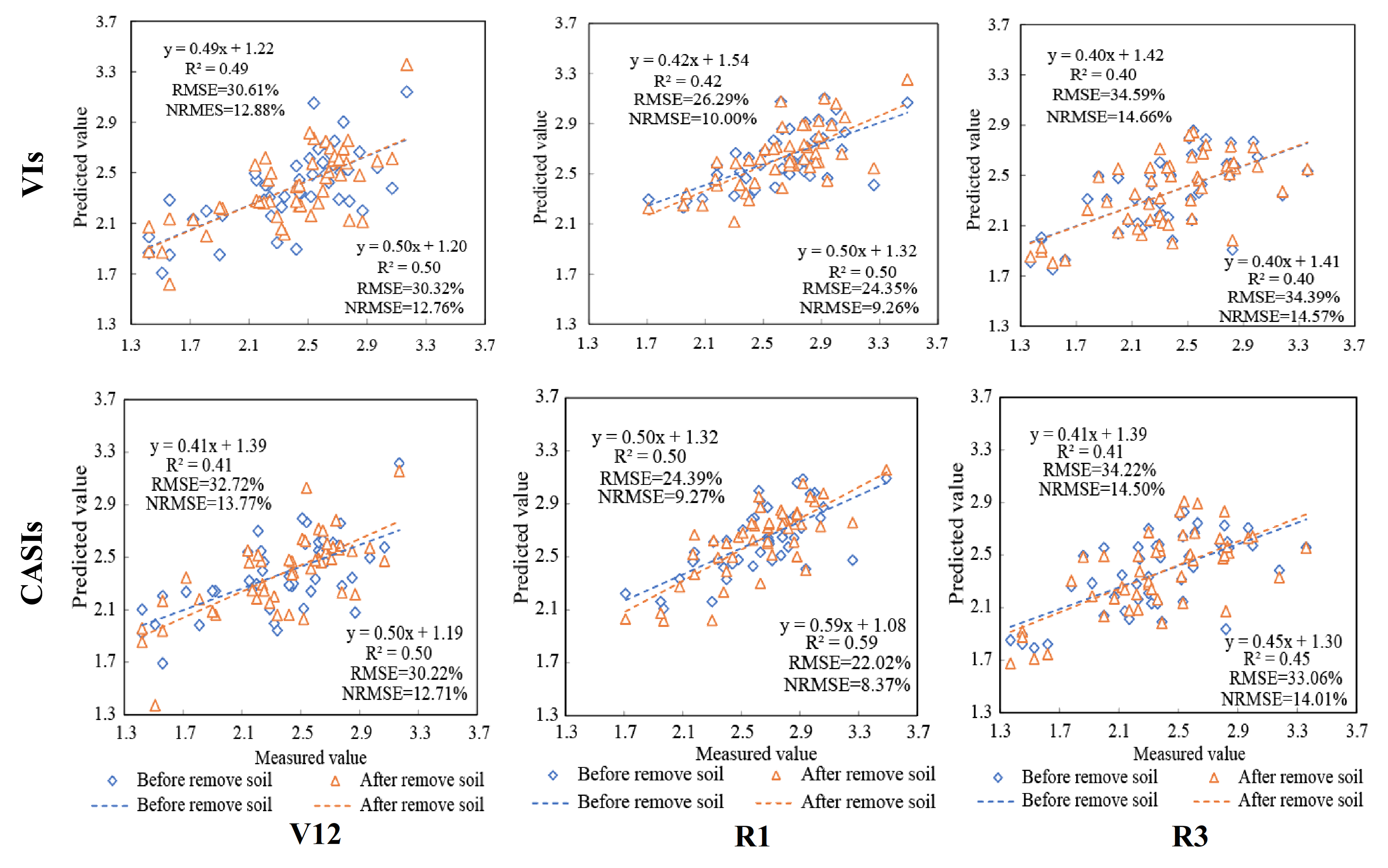
3.3. Estimation of LNC in Corn Using CASIs and VIs

Based on the above optimal features selected by RFA in each growth stage, PLSR was used to estimate LNC in corn. Figure 5 shows the relationships between the predicted and measured LNC using VIs without and with removing soil noise in the different stages. It can be seen that the estimations of LNC with removal of soil noise are generally better than those without eliminating soil noise, which indicates it is necessary for assessing nitrogen status to take soil influence into account.

Unlike VIs using only multispectral images from UAV, CASIs which were constructed by adding the factor, ${\mathrm{FV}}_{\mathrm{cover}}$, to VIs were extracted to estimate LNC in corn using UAV RGB and multispectral images in this study. Figure 5 shows that the CASIs had a better performance after soil elimination than before soil removal, with the best R² of 0.59, RMSE of 22.02%, and NRMSE of 8.37% in the R1 stage. What is more, it can be seen from

Table 6. Comparison using optimal CASIs and VIs to evaluate LNC in different growth stages, with different processing for the soil background.

Conditions	Stages	CASI			VI
		R2	RMSE	NRMSE	R2	RMSE	NRMSE
No removal of soil	V12	0.41	32.72%	13.77%	0.49	30.61%	12.88%
	R1	0.50	24.39%	9.27%	0.42	26.29%	10.00%
	R3	0.41	34.22%	14.50%	0.40	34.59%	14.66%
Soil removal	V12	0.50	30.22%	12.71%	0.50	30.32%	12.76%
	R1	0.59	22.02%	8.37%	0.50	24.35%	9.26%
	R3	0.45	33.06%	14.01%	0.40	34.39%	14.57%

that the CASIs generally exhibited the better capability for estimating LNC than the Vis, whether removing background soil or not.

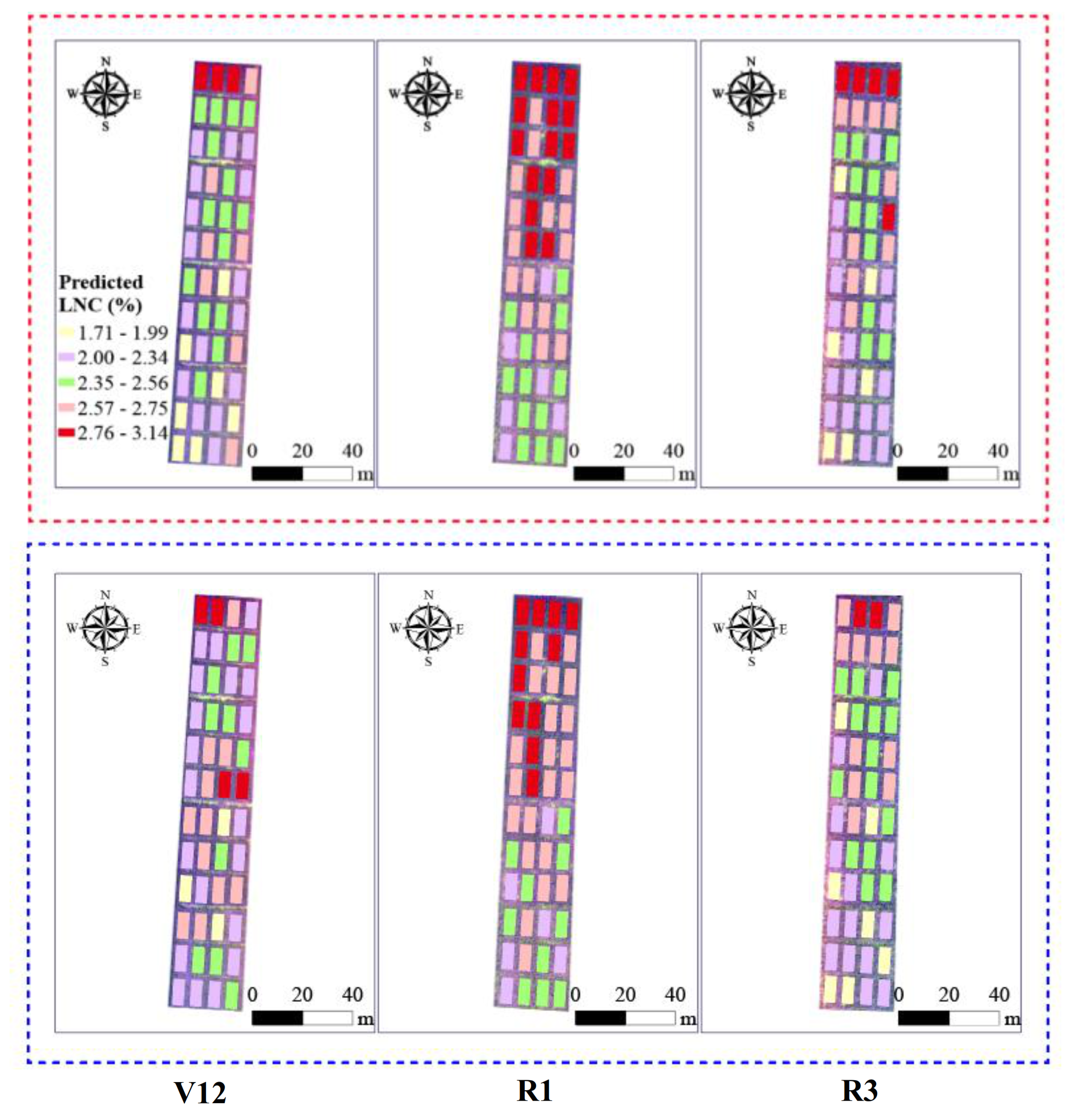
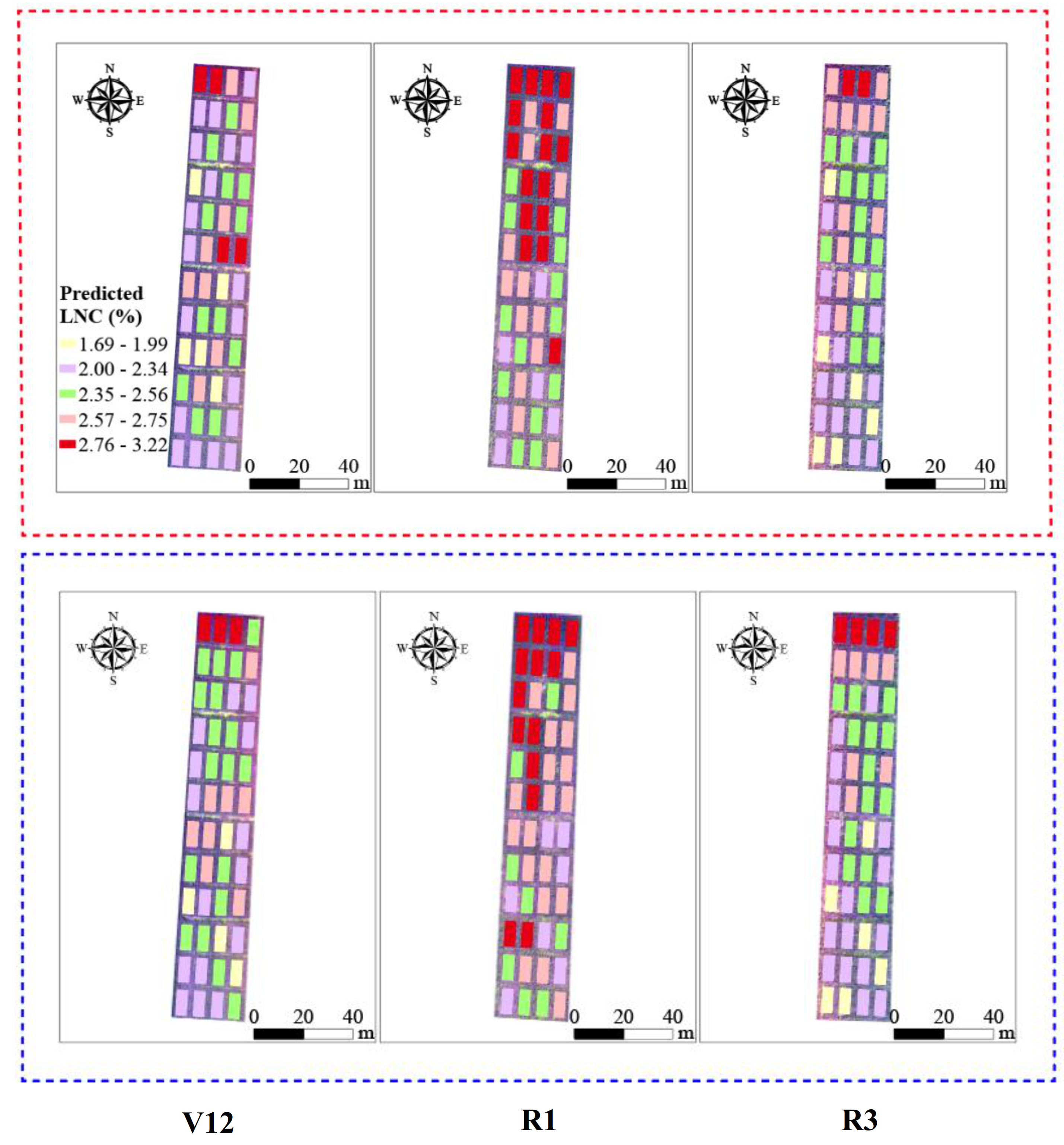
3.4. Mapping LNC Based on UAV Images at Plot Scale

VIs at different growth stages of corn were extracted from UAV multispectral images covering the 48 plots. The best five were selected by RFA from VIs to establish the PLSR model for LNC estimates, and then the LNC distributions at plot scale were mapped for each stage (Figure 6). The mapping analysis results show that although there was the same nitrogen treatment (N2) at the 24 plots in the northern study area, LNC in the three stages still ranges from 2.00% to 3.14% due to trait differences among cultivars, and this situation is similar whether soil noise is removed or not. In addition, it can also be noticed that the LNC at the same cultivar plots shows an obvious consistency in the R1 stage, which also happens in this stage after soil elimination. This may be because corn in the R1 stage is the most vigorous, vegetation coverage is also the largest, and soil has the least influence on the corn canopies.

At the 24 plots in the southern study area, the different nitrogen application rates resulted in distinct differences in corn growth. LNC ranged greatly from 1.71% to 2.75% in the V12 and R3 stage, and only from 2.00% to 2.75% in R1 stage. It can be seen from Figure 6 that after eliminating soil background, LNC changes at plot scale were more consistent with nitrogen treatments in comparison with no soil removal.

The five sensitive CASIs using UAV RGB and multispectral images were selected by RFA to construct the models for estimating LNC based on PLSR, and LNC distributions for each stage were mapped at plot scale (Figure 7). Like VI-based LNC distributions, LNC using CASI at the northern 24 plots in the three stages ranged greatly from 1.69% to 3.22% due to cultivar differences, even if there was the same nitrogen treatment; this was particularly evident in the V12 and R3 stages, and only in the R1 stage LNC shows some consistency at the same cultivar plots. Comparing with no soil removal, LNC with soil elimination at the northern plots slightly increased.

In the southern plots, corn growth in the three stages was closely related to nitrogen treatment. High nitrogen application rates (N2 and N3) indicated better growth with high LNC for corn, no nitrogen treatment (N0) showed the worst growth. From Figure 7, it can be seen that LNC changed at plot scale, consistent with nitrogen treatments generally, and it was more distinct in the R1 stage after soil removal. In addition, corn growth in the R1 stage was the most vigorous among the three stages, which was well reflected by the LNC distribution in the R1 stage.

4. Discussion

4.1. Partial Soil or Shadow Removal on UAV Images

Compared with satellite remote-sensing images, the low-altitude UAV images have a higher spatial resolution, and the vegetation textures in images are also more prominent, however, there is also much more soil or shadow background in UAV-based images. Low-altitude UAV remote-sensing images are strongly affected by planting density, row distance, canopy structure, and other factors, but these factors are usually linked with the soil [16,51]. For instance, lower crop planting density will lead to lower vegetation coverage, and the soil background and shadow will certainly increase in images. Hence, the problem of how to alleviate the influence from soil or shadow noise must inevitably be considered in UAV applications. In previous studies, RGB images have been usually converted into HSV color space for soil and shadow detection [52,53,54]. In this study, HSV color transformation was applied for the elimination of soil and shadow background from UAV RGB images, and this indicates that it is very effective to remove soil or shadow by HSV. Particularly, HSV was consecutively used two times in this study, and the soil and shadow could be clearly identified in the HSV2 images (Figure 2), which may have a certain significance for the other related studies.

4.2. Vegetation Features for LNC Evaluates

Vegetation indices (VIs) derived from the combination of characteristic bands in multispectral data can highlight the properties of vegetation, and be widely used for estimating crop parameters, such as nitrogen and chlorophyll content [48,49,55]. However, VIs are usually affected by many factors, and exhibit different traits. Some have great potential for suppressing soil noise [16,34], and others are good at anti-saturation for vegetation spectra [36,41]. Therefore, effectively selecting sensitive features from VIs to assess nitrogen status should be considered [10,56,57]. In the present study, the random frog algorithm (RFA) was implemented to select a set of the sensitive features from UAV images to estimate LNC in the V12, R1, and R3 stages of corn. Among the sets of sensitive features for the three stages, the red-edge (REG) and near infrared (NIR) band features were significantly selected for LNC estimates; the two features had also been used to predict maize LNC in an existing report [10]. In practice, REG is one of the most widely used spectral features for evaluating crop parameters [39,55,56,57,58,59] and NIR is also the key component for most typical VIs [16,31,32,33,34,35,36,37,38,39,40,41,42,43].

CASI is actually a kind of VI, just adding the parameter of vegetation cover, ${\mathrm{FV}}_{\mathrm{cover}}$, to the conventional VI. Compared with VIs, CASIs had generally better correlations with LNC in this study, which is in line with a previous study [19]. The existing research has demonstrated that soil background can greatly influence the relationships between canopy spectra and N status [19,60,61,62]. The Addition of ${\mathrm{FV}}_{\mathrm{cover}}$ to the basis of VI should be a good method for eliminating the influence of soil, which should make CASI more sensitive to nitrogen status in crops. In addition, it should be noted that in this study the elimination of soil noise was applied only for UAV multispectral images with relatively low spatial resolution. Despite soil removal from multispectral images by threshold segmentation, there were still mixed pixels with soil and vegetation cover derived from UAV RGB images with higher spatial resolution; CASIs integrating VI with FV_cover should be able to further eliminate some noise after removing soil noise.

4.3. Advantages and Disadvantages of UAV Data Applications

There have been some reports where UAV images from multiple sensors were simultaneously implemented to estimate crop parameters, and in these studies the images from different sensors were often used to individually extract a variety of spectral variables, then the variables were directly input into various models for evaluating crop growth status, while little attention has been paid to the application of a fusion of information from images of different sensors [10,14,63]. In this study, high-definition RGB images were used to efficiently extract vegetation coverage (${\mathrm{FV}}_{\mathrm{cover}}$) in plots, and multispectral images for the calculation of typical vegetation indices (VIs), then CASIs that integrate VIs with ${\mathrm{FV}}_{\mathrm{cover}}$ were acquired to estimate LNC in corn. CASIs can make good use of the complementary advantages from two types of UAV images, and are a simple and effective method of information fusion. In fact, it is a developing trend to use a fusion of information for crop growth assessment [64].

However, there are still some deficiencies that need to be improved further. Due to the influence of the shooting angles and solar-irradiance angles on low-altitude UAV, some soil and shadow could not be completely removed. The training models constructed in this study only used data in three stages of one year. Thus, further validation will be needed using data from many years or different areas in the future.

5. Conclusions

This study explored how to use digital RGB and multispectral images from two sensors mounted simultaneously on a low-altitude UAV to assess nitrogen status in three growth stages of corn. CASIs that connect VIs with vegetation cover (${\mathrm{FV}}_{\mathrm{cover}}$) used the UAV images from two sensors to estimate LNC in corn based on the PLS with RFA methods. The results proved that CASIs exhibited the better estimation of LNC in comparison with VIs in all of the three growth stages of corn, regardless of soil removal. It is concluded that CASIs fusing useful information from both digital RGB and multispectral images acquired synchronously by UAV appear very promising, and have potential for remotely monitoring leaf nitrogen content in crops. The preliminary research of using CASIs can also provide new ideas and referential methods for UAV monitoring of other biochemical parameters.

References

1. Fitzgerald, G.; Rodriguez, D.; O’Leary, G. Measuring and predicting canopy nitrogen nutrition in wheat using a spectral index—The canopy chlorophyll content index (CCCI). Field Crop. Res. 2010, 116, 318–324. [Google Scholar] [CrossRef]
2. Xue, L.; Luo, W.; Cao, W.; Tian, Y. Research progress on the water and nitrogen detection using spectral reflectance. Int. J. Remote Sens. 2003, 7, 73–80. [Google Scholar]
3. Tremblay, N. Determining nitrogen requirements from crops characteristics. Benefits and challenges. In Recent Research Development Agronomy and Horticultur, 1st ed.; Pandalai, S.G., Ed.; Research Signpost: Kerala, India, 2004; pp. 157–182. [Google Scholar]
4. Mulla, D.J. Twenty five years of remote sensing in precision agriculture: Key advances and remaining knowledge gaps. Biosyst. Eng. 2013, 114, 358–371. [Google Scholar] [CrossRef]
5. Ballesteros, R.; Ortega, J.F.; Hernandez, D.; Moreno, M.A. Applications of georeferenced high-resolution images obtained with unmanned aerial vehicles. Part I: Description of image acquisition and processing. Precis. Agric. 2014, 15, 579–592. [Google Scholar] [CrossRef]
6. Peña, J.M.; Torres-Sánchez, J.; de Castro, A.I.; Kelly, M.; López-Granados, F. Weed mapping in early-season maize fields using object-based analysis of Unmanned Aerial Vehicle (UAV) images. PLoS ONE 2013, 8, e77151. [Google Scholar] [CrossRef] [Green Version]
7. Swain, K.C.; Thomson, S.J.; Jayasuriya, H.P.W. Adoption of an unmanned helicopter for low-altitude remote sensing to estimate yield and total biomass of a rice crop. Trans. ASABE 2010, 53, 21–27. [Google Scholar] [CrossRef] [Green Version]
8. Shamshiri, R.R.; Hameed, I.A.; Balasundram, S.K.; Ahmad, D.; Weltzien, C.; Yamin, M. Fundamental Research on Unmanned Aerial Vehicles to Support Precision Agriculture in Oil Palm Plantations. In Agricultural Robots-Fundamentals and Applications, 1st ed.; Zhou, J., Ed.; IntechOpen: Nanjing, China, 2019; pp. 91–116. [Google Scholar]
9. Swain, K.C.; Jayasuriya, H.P.W.; Salokhe, V.M. Suitability of low-altitude remote sensing images for estimating nitrogen treatment variations in rice cropping for precision agriculture adoption. J. Appl. Remote Sens. 2007, 1, 6656–6659. [Google Scholar] [CrossRef]
10. Osco, L.P.; Junior, J.M.; Ramos, A.P.M.; Furuya, D.E.G.; Santana, D.C.; Teodoro, L.P.R.; Gonçalves, W.N.; Baio, F.H.R.; Pistori, H.; Junior, C.A.D.S.; et al. Leaf nitrogen concentration and plant height prediction for maize using UAV-based multispectral imagery and machine learning techniques. Remote Sens. 2020, 12, 3237. [Google Scholar] [CrossRef]
11. Lee, H.; Wang, J.; Leblon, B. Using linear regression, Random Forests, and Support Vector Machine with unmanned aerial vehicle multispectral images to predict canopy nitrogen weight in corn. Remote Sens. 2020, 12, 2071. [Google Scholar] [CrossRef]
12. Liu, H.; Zhu, H.; Wang, P. Quantitative modelling for leaf nitrogen content of winter wheat using UAV-based hyperspectral data. Int. J. Remote Sens. 2017, 38, 2117–2134. [Google Scholar] [CrossRef]
13. Lu, J.; Cheng, D.; Geng, C.; Zhang, Z.; Xiang, Y.; Hu, T. Combining plant height, canopy coverage and vegetation index from UAV-based RGB images to estimate leaf nitrogen concentration of summer maize. Biosyst. Eng. 2021, 202, 42–54. [Google Scholar] [CrossRef]
14. Kefauver, S.C.; Vicente, R.; Vergara-Díaz, O.; Fernandez-Gallego, J.A.; Kerfal, S.; Lopez, A. Comparative UAV and field phenotyping to assess yield and nitrogen use efficiency in hybrid and conventional barley. Front. Plant Sci. 2017, 8, 1733. [Google Scholar] [CrossRef] [PubMed]
15. Huete, A.; Jackson, R.D.; Post, D.F. Spectral response of a plant canopy with different soil backgrounds. Remote Sens. Environ. 1985, 17, 37–53. [Google Scholar] [CrossRef]
16. Rondeaux, G.; Steven, M.D.; Baret, F. Optimization of soil adjusted vegetation indices. Remote Sens. Environ. 1996, 55, 95–107. [Google Scholar] [CrossRef]
17. Major, D.; Frederic, B.; Guyot, G. A ratio vegetation index adjusted for soil brightness. Int. J. Remote Sens. 1990, 11, 727–740. [Google Scholar] [CrossRef]
18. Liu, S.; Yang, G.; Jing, H.; Feng, H.; Li, H.; Chen, P.; Yang, W. Retrieval of winter wheat nitrogen content based on UAV digital image. Trans. CSAE 2019, 35, 75–85, (In Chinese with English Abstract). [Google Scholar]
19. Yao, X.; Ren, H.; Cao, Z.; Tian, Y.; Cao, W.; Zhu, Y.; Cheng, T. Detecting leaf nitrogen content in wheat with canopy hyperspectrum under different soil backgrounds. Int. J. Appl. Earth Obs. Geoinf. 2014, 32, 114–124. [Google Scholar] [CrossRef]
20. Ritchie, S.W.; Hanway, J.J. How a Corn Plant Develops; Special Report No. 48; Iowa State University of Science and Technology, Cooperative Extension Service: Ames, IA, USA, 1986; pp. 1–21. [Google Scholar]
21. Tsai, C.M.; Yeh, Z.M. Contrast enhancement by automatic and parameter-free piecewise linear transformation for color images. IEEE Trans. Consum. Electron. 2008, 54, 213–219. [Google Scholar] [CrossRef] [Green Version]
22. Guo, P.; Wu, F.; Dai, J.; Wang, H.; Xu, L.; Zhang, G. Comparison of farmland crop classification methods based on visible light images of unmanned aerial vehicles. Trans. CSAE 2017, 33, 112–119, (In Chinese with English Abstract). [Google Scholar]
23. Vimal, C.; Sathish, B. Random Forest Classifier Based ECG Arrhythmia Classification. Int. J. Healthc. Inf. Syst. Inform. 2010, 5, 1–10. [Google Scholar] [CrossRef]
24. Torres, M.; Qiu, G.P. Automatic habitat classification using image analysis and random forest. Ecol. Inform. 2014, 23, 126–136. [Google Scholar] [CrossRef]
25. Akar, Ö.; Güngör, O. Classication of multispectral images using Random Forest algorithm. J. Geod. Geoinf. 2012, 1, 105–112. [Google Scholar] [CrossRef] [Green Version]
26. Li, C.; Wang, J.; Liu, L.; Wang, R. Automated digital image analyses for estimating percent ground cover of winter wheat based on object features. J. Zhejiang Univ. Agric. Life Sci. 2004, 30, 650–656, (In Chinese with English Abstract). [Google Scholar]
27. Jia, J.; Hu, Y.; Liu, L. Useing Digital Photography to Measure Vegetation Coverage in Qinghai-Tibet Plateau. J. Geoinf. Sci. 2010, 12, 880–885, (In Chinese with English Abstract). [Google Scholar]
28. Zhang, J.; Pu, R.; Yuan, L. Integrating remotely sensed and meteorological observations to forecast wheat powdery mildew at a regional scale. IEEE J. Sel. Top. Appl. Earth Obs. Remote Sens. 2014, 7, 4328–4339. [Google Scholar] [CrossRef]
29. Fan, L.; Zhao, J.; Xu, X.; Liang, D.; Yang, G.; Feng, H.; Yang, H.; Yulong, W.; Chen, G.; Wei, P. Hyperspectral-based estimation of leaf nitrogen content in corn using optimal selection of multiple spectral variables. Sensors 2019, 19, 2898. [Google Scholar] [CrossRef] [Green Version]
30. Xu, X.; Zhao, C.; Wang, J.; Zhang, J.; Song, X. Using optimal combination method and in situ hyperspectral measurements to estimate leaf nitrogen concentration in barley. Precis. Agric. 2014, 15, 227–240. [Google Scholar] [CrossRef]
31. Richardson, A.J.; Wiegand, C.L. Distinguishing vegetation from soil background information. Photogramm. Eng. Remote Sens. 1977, 43, 1541–1552. [Google Scholar]
32. Gitelson, A.; Kaufman, Y.J.; Merzlyak, M.N. Use of a green channel in remote sensing of global vegetation from EOS-MODIS. Remote Sens. Environ. 1996, 58, 289–298. [Google Scholar] [CrossRef]
33. Gong, P.; Pu, R.; Biging, G.S.; Larrieu, M.R. Estimation of forest leaf area index using vegetation indices derived from Hyperion hyperspectral data. IEEE Trans. Geosci. Remote Sens. 2003, 41, 1355–1362. [Google Scholar] [CrossRef] [Green Version]
34. Qi, J.G.; Chehbouni, A.; Huete, A.; KERR, Y.; Sorooshian, S. A modified soil adjusted vegetation index. Remote Sens. Environ. 1994, 48, 119–126. [Google Scholar] [CrossRef]
35. Chen, J.M. Evaluation of vegetation indices and a modified simple ratio for boreal applications. Can. J. Remote Sens. 1996, 22, 229–242. [Google Scholar] [CrossRef]
36. Haboudane, D.; Miller, J.R.; Pattey, E.; Zarco-Tejada, P.J.; Strachan, I.B. Hyperspectral vegetation indices and novel algorithms for predicting green LAI of crop canopies: Modeling and validation in the context of precision agriculture. Remote Sens. Environ. 2004, 90, 337–352. [Google Scholar] [CrossRef]
37. Rouse, J.W.; Haas, R.H.; Schell, J.A.; Deering, D.W. Monitoring Vegetation Systems in the Great Plains with ERTS. In Proceedings of the Third ERTS Symosium, Washington, DC, USA, 10–14 December 1973; Volume 1, pp. 48–62. [Google Scholar]
38. Goel, N.S.; Qin, W. Influences of canopy architecture on relationships between various vegetation indices and LAI and Fpar: A computer simulation. Remote Sens. Rev. 1994, 10, 309–347. [Google Scholar] [CrossRef]
39. Gitelson, A.A.; Viña, A.; Ciganda, V.; Rundquist, D.C.; Arkebauer, T.J. Remote estimation of canopy chlorophyll content in crops. Geophys. Res. Lett. 2005, 32, L08403. [Google Scholar] [CrossRef] [Green Version]
40. Roujean, J.L.; Bŕeon, F.M. Estimating PAR absorbed by vegetation from bidirectional reflectance measurements. Remote Sens. Environ. 1995, 51, 375–384. [Google Scholar] [CrossRef]
41. Jordan, C.F. Derivation of Leaf Area Index from Quality of Light on the Forest Floor. Ecology 1969, 50, 663–666. [Google Scholar] [CrossRef]
42. Xue, L.H.; Cao, W.X.; Luo, W.H.; Dai, T.B.; Zhu, Y. Monitoring leaf nitrogen status in rice with canopy spectral reflectance. Agron. J. 2004, 96, 135–142. [Google Scholar] [CrossRef]
43. Broge, N.H.; Leblanc, E. Comparing prediction power and stability of broadband and hyperspectral vegetation indices for estimation of green leaf area index and canopy chlorophyll density. Remote Sens. Environ. 2001, 76, 156–172. [Google Scholar] [CrossRef]
44. Li, H.; Xu, Q.; Liang, Y. Random Frog: An efficient reversible jump Markov Chain Monte Carlo-like approach for variable selection with applications to gene selection and disease classification. Anal Chim. Acta 2012, 740, 20–26. [Google Scholar] [CrossRef]
45. Hu, M.H.; Zhai, G.T.; Zhao, Y.; Wang, Z.D. Uses of selection strategies in both spectral and sample spaces for classifying hard and soft blueberry using near infrared data. Sci. Rep. 2018, 8, 6671. [Google Scholar] [CrossRef] [PubMed] [Green Version]
46. Zhang, C.; Kong, W.; Liu, F.; He, Y. Measurement of aspartic acid in oilseed rape leaves under herbicide stress using near infrared spectroscopy and chemometrics. Heliyon 2016, 2, e00064. [Google Scholar] [CrossRef] [PubMed] [Green Version]
47. Wold, S.; Ruhe, A.; Wold, H.; Dunn, W.J., III. The collinearity problem in linear regression. The partial least squares (PLS) approach to generalized inverses. SIAM J. Sci. Stat. Comput. 1984, 5, 735–743. [Google Scholar] [CrossRef] [Green Version]
48. Li, F.; Mistele, B.; Hu, Y.; Chen, X.; Schmidhalter, U. Reflectance estimation of canopy nitrogen content in winter wheat using optimised hyperspectral spectral indices and partial least squares regression. Eur. J. Agron. 2014, 52, 198–209. [Google Scholar] [CrossRef]
49. Hunt, E.R., Jr.; Doraiswamy, P.C.; McMurtrey, J.E.; Daughtry, C.S.T.; Perry, E.M.; Akhmedov, B. A visible band index for remote sensing leaf chlorophyll content at the canopy scale. Int. J. Appl. Earth Obs. Geoinf. 2013, 21, 103–112. [Google Scholar] [CrossRef] [Green Version]
50. Cho, M.A.; Skidmore, A.K. A new technique for extracting the red edge position from hyperspectral data: The linear extrapolation method. Remote Sens. Environ. 2006, 101, 181–193. [Google Scholar] [CrossRef]
51. Rasmussen, J.; Ntakos, G.; Nielsen, J.; Svensgaard, J.; Poulsenb, R.N.; Christensena, S. Are vegetation indices derived from consumer-grade cameras mounted on UAVs sufficiently reliable for assessing experimental plots? Eur. J. Agron. 2016, 74, 75–92. [Google Scholar] [CrossRef]
52. Farou, B.; Rouabhia, H.E.; Seridi, H.; Akdag, H. Novel approach for detection and removal of moving cast shadows based on RGB, HSV and YUV color spaces. Comput. Inform. 2017, 36, 837–856. [Google Scholar] [CrossRef]
53. Surkutlawar, S.; Kulkarni, R.K. Shadow suppression using RGB and HSV color space in moving object detection. Int. J. Adv. Comput. Sci. Appl. 2013, 4, 164. [Google Scholar]
54. Zhang, Y.; Hartemink, A.E. A method for automated soil horizon delineation using digital images. Geoderma 2019, 343, 97–115. [Google Scholar] [CrossRef]
55. Li, F.; Miao, Y.; Feng, G.; Yuan, F.; Yue, S.; Gao, X.; Liu, Y.; Liu, B.; Ustin, S.L.; Chen, X. Improving estimation of summer maize nitrogen status with red edge-based spectral vegetation indices. Field Crop. Res. 2014, 157, 111–123. [Google Scholar] [CrossRef]
56. Osco, L.P.; Ramos, A.P.M.; Pinheiro, M.M.F.; Moriya, É.A.S.; Imai, N.N.; Estrabis, N.; Ianczyk, F.; de’Araújo, F.F.; Liesenberg, V.; de Castro Jorge, L.A.; et al. A machine learning approach to predict nutrient content in valencia-orange leaf hyperspectral measurements. Remote Sens. 2020, 12, 906. [Google Scholar] [CrossRef] [Green Version]
57. Zheng, H.; Li, W.; Jiang, J.; Liu, Y.; Cheng, T.; Tian, Y.; Zhu, Y.; Cao, W.; Zhang, Y.; Yao, X. A comparative assessment of different modeling algorithms for estimating leaf nitrogen content in winter wheat using multispectral images from an unmanned aerial vehicle. Remote Sens. 2018, 10, 2026. [Google Scholar] [CrossRef] [Green Version]
58. Dong, T.; Liu, J.; Shang, J.; Qian, B.; Ma, B.; Kovacs, J.M.; Walters, D.; Jiao, X.; Geng, X.; Shi, Y. Assessment of red-edge vegetation indices for crop leaf area index estimation. Remote Sens. Environ. 2019, 222, 133–143. [Google Scholar] [CrossRef]
59. Fu, Y.; Yang, G.; Li, Z.; Li, H.; Li, Z.; Xu, X.; Song, X.; Zhang, Y.; Duan, D.; Zhao, C.; et al. Progress of hyperspectral data processing and modelling for cereal crop nitrogen monitoring. Comput. Electron. Agric. 2020, 172, 105321. [Google Scholar] [CrossRef]
60. Sun, L.; Cheng, L. Anti-soil background capacity with vegetation biochemicalcomponent spectral model. Acta Ecol. Sin. 2011, 31, 1641–1652. [Google Scholar]
61. Gilabert, M.; González-Piqueras, J.; Garcııa-Haro, F.; Meliá, J. A generalized soil-adjusted vegetation index. Remote Sens. Environ. 2002, 82, 303–310. [Google Scholar] [CrossRef]
62. Chen, P.; Haboudane, D.; Tremblay, N.; Wang, J.; Vigneault, P.; Li, B. New spectral indicator assessing the efficiency of crop nitrogen treatment in corn and wheat. Remote Sens. Environ. 2010, 114, 1987–1997. [Google Scholar] [CrossRef]
63. Maimaitijiang, M.; Sagan, V.; Sidike, P.; Daloye, A.M.; Erkbol, H.; Fritschi, F.B. Crop Monitoring Using Satellite/UAV Data Fusion and Machine Learning. Remote Sens. 2020, 12, 1357. [Google Scholar] [CrossRef]
64. Maimaitijiang, M.; Sagan, V.; Sidike, P.; Hartling, S.; Esposito, F.; Fritschi, F.B. Soybean yield prediction from UAV using multimodal data fusion and deep learning. Remote Sens. Environ. 2020, 237, 111599. [Google Scholar] [CrossRef]
Figure 1. Location of the study area and experimental design.
Remotesensing 13 00340 g001
Figure 2. Spatial distribution maps of RGB images with color transformation in three different stages (V12, R1, and R3): (1) original RGB images in the study area, (2) hue saturation value (HSV) primary transformation, and (3) HSV secondary transformation, respectively.
Remotesensing 13 00340 g002
Figure 3. Flowchart illustrating the extraction of coverage adjusted spectral indices (CASI) with unmanned aerial vehicle (UAV) multispectral and RGB images.
Remotesensing 13 00340 g003
Figure 4. Relationships between VIs, CASIs, and LNC in the three stages of V12, R1, and R3. (a,b) denote the correlations between VIs and LNC before and after removing the soil background, respectively. (c,d) refer to the correlations between CASIs and LNC before and after soil removal, respectively.
Remotesensing 13 00340 g004
Figure 5. Relationships between the predicted and measured values of LNC using optimal VIs and CASIs selected by RFA before and after removing soil noise in the three stages of V12, R1, and R3.
Remotesensing 13 00340 g005
Figure 6. LNC distribution maps of corn using VIs from UAV multispectral images at plot scale in the three stages of V12, R1, and R3. The distribution maps of LNC without soil removal are shown in the red dotted box, those with eliminating soil are in the blue dotted box.
Remotesensing 13 00340 g006
Figure 7. Distribution maps of LNC in corn based on CASIs using UAV RGB and multispectral images at plot scale in the three stages of V12, R1, and R3. The maps of LNC without soil removal are shown in the red dotted box, and those with soil removal are in the blue dotted box.
Remotesensing 13 00340 g007