Article

Assessing the Potential of the DART Model to Discrete Return LiDAR Simulation—Application to Fuel Type Mapping

by
Sergio Revilla
1,2,
María Teresa Lamelas
2,3,*,†,
Darío Domingo
2,4,†,
Juan de la Riva
2,
Raquel Montorio
2,
Antonio Luis Montealegre
2 and
Alberto García-Martín
2,3
1
Instituto Geográfico de Aragón, Pº María Agustín, 36, Edificio Pignatelli, 50071 Zaragoza, Spain
2
GEOFOREST-IUCA Research Group, Department of Geography, University of Zaragoza, Pedro Cerbuna 12, 50009 Zaragoza, Spain
3
Centro Universitario de la Defensa de Zaragoza, Academia General Militar, Ctra. de Huesca s/n, 50090 Zaragoza, Spain
4
Land Change Science Research Unit, Swiss Federal Institute for Forest, Snow and Landscape Research WSL, Zurcherstrasse 111, 8930 Birmensdorf, Switzerland
*
Author to whom correspondence should be addressed.
These authors contributed equally to this work.
Remote Sens. 2021, 13(3), 342; https://doi.org/10.3390/rs13030342
Submission received: 11 December 2020 / Revised: 13 January 2021 / Accepted: 16 January 2021 / Published: 20 January 2021
(This article belongs to the Special Issue Feature Paper Special Issue on Forest Remote Sensing)

Abstract

:
Fuel type is one of the key factors for analyzing the potential of fire ignition and propagation in agricultural and forest environments. The increase of three-dimensional datasets provided by active sensors, such as LiDAR (Light Detection and Ranging), has improved the classification of fuel types through empirical modelling. Empirical methods are site and sensor specific while Radiative Transfer Models (RTM) approaches provide broader universality. The aim of this work is to analyze the suitability of Discrete Anisotropic Radiative Transfer (DART) model to replicate low density small-footprint Airborne Laser Scanning (ALS) measurements and subsequent fuel type classification. Field data measured in 104 plots are used as ground truth to simulate LiDAR response based on the sensor and flight characteristics of low-density ALS data captured by the Spanish National Plan for Aerial Orthophotography (PNOA) in two different dates (2011 and 2016). The accuracy assessment of the DART simulations is performed using Spearman rank correlation coefficients between the simulated metrics and the ALS-PNOA ones. The results show that 32% of the computed metrics overpassed a correlation value of 0.80 between simulated and ALS-PNOA metrics in 2011 and 28% in 2016. The highest correlations were related to high height percentiles, canopy variability metrics as for example standard deviation and Rumple diversity index, reaching correlation values over 0.94. Two metric selection approaches and Support Vector Machine classification method with variants were compared to classify fuel types. The best-fitted classification model, trained with the DART simulated sample and validated with ALS-PNOA data, was obtained using Support Vector Machine method with radial kernel. The overall accuracy of the classification after validation was 88% and 91% for the 2011 and 2016 years, respectively. The use of DART demonstrates its value for simulating generalizable 3D data for fuel type classification providing relevant information for forest managers in fire prevention and extinction.

Graphical Abstract

1. Introduction

Fuel types are defined by Merrill and Alexander [1] as “an identifiable association of fuel elements of distinctive species, form, size, arrangement and continuity that will exhibit characteristic fire behavior under defined burning conditions.” Fuel type mapping is crucial for forest management and fire risk assessment as the spatial distribution of fuel affects wildfire ignition and propagation.
Historically, forest fires have had a relevant impact in Mediterranean landscapes, however, in the last decades, the recurrence, magnitude and severity of wildfires have increased [2]. In addition to other factors derived from climate change, for example, the increase in temperature, one of the main driving forces of this fire occurrence intensification is the increase of vegetation combustibility because of land use and cover changes [2,3]. The abandonment of the field crops leads to the proliferation of bushes increasing the fuel load [4]. Consequently, fuel type mapping has been accomplished by several authors using remote sensed data [4,5], mostly based on multispectral medium-resolution sensors [5,6,7,8] but also using hyperspectral images captured by sensors on board of aircrafts [9,10], airborne and satellite LiDAR (Light Detection and Ranging) data [11,12,13] and the combination of different types of sensors [14,15,16,17,18,19].
The development of LiDAR technology constitutes an important advance in forest management through remote sensing techniques [20] due to the possibility of capturing the vegetation vertical profile; contrarily to multispectral imagery from optical passive sensors, only sensitive to the upper canopy [21,22]. However, most of the abovementioned approaches to classifying fuel types, independently from the remote sensing technology used, rely on in situ data to train algorithms using statistical approaches [23]. These empirical methods are site and sensor specific and their results are only applicable to fuel types present in the study area [24]. An alternative approach involves model training through radiative transfer simulations of the terrain characteristics. These simulations can provide a cost-effective alternative to field surveys while improving the control in the experiments [25]. Radiative Transfer Models (RTM) approaches are subject to an appropriate model parameterization that also requires in situ data, however they offer a better universality than empirical approaches [26].
Previous forest parameter simulations conducted with 3D RTM capable of simulating the LiDAR response, such as FLIGHT [27] and Discrete Anisotropic Radiative Transfer (DART) [28] models, have mainly focused on large-footprint waveform LiDAR acquisitions from satellite [29,30] or onboard aircraft [24,26,31]. However, few investigations have examined small-footprint discrete-return measurements due to the computational demands of simulating multi-pulse ALS acquisitions over complex forested landscapes. From the best of our knowledge, the only study available was conducted by Roberts et al. [25]. These authors examined the accuracy of the DART model to replicate small-footprint ALS measurements collected over Irish conifer plantations and how survey characteristics influenced the precision of discrete-return metrics. Their study demonstrated that DART is a robust model for simulating high point density (a mean point density of 29 ± 10 returns/m2) discrete-return measurements over structurally complex forests, opening a promising line of research.
Today, several countries, such as Austria, Canada, Denmark, Estonia, England, Finland, Ireland, Lithuania, Luxemburg, Malta, Norway, Spain, Slovakia, Switzerland, The Netherlands and the United States of America, have nationwide ALS data coverages [32] available for free in the Internet. Point clouds derived from such national campaigns generally are captured by small-footprint (<1 m) pulsed laser systems capable of recording a finite number of discrete returns (typically <5) per laser pulse and have low point densities in order to reduce costs [33]. One of the purposes of these campaigns is to derive different forestry variable mapping at regional scale with an operational objective. The regional or national scale of these projects makes even more impractical to quantify directly in situ data through conventional forest mensuration techniques.
In order to overcome this handicap, the specific objectives of the present study are: 1. To analyze the accuracy of the DART model to replicate low density small-footprint ALS measurements 2. To assess the ability of simulations for model training to classify fuel types. Although, the ability of the DART model to classify fuel models was assessed by Lamelas et al. [24], this approach represents the first attempt to simulate the response of low density small-footprint sensors for fuel classification.
The results of this study are important for operational forestry as could imply a considerable decrease in the human and economic resources invested in the field surveys conducted to forest variable mapping.

2. Material

2.1. Study Area

The study area is located in the central part of Ebro valley (41°50’ N, 0º57’ W) (Figure 1), northeast of Spain. The forest under study corresponds to monospecific stands of Pinus halepensis Mill. fragmented in stands of variable sizes and occupies approximately 8000 ha. In some areas, Aleppo pine forest is interspersed with evergreen shrubs, dominated by Quercus coccifera L., Juniperus oxycedrus L. subsp. macrocarpa (Sibth. & Sm.) Ball and Thymnus vulgaris L. Part of the study area is located inside the Military Training Center (CENAD) “San Gregorio,” involving a direct risk of fire [34].
Aleppo pine forests play an important role in the protection and recovery of forest in Mediterranean region characterized by nutrient-poor, gypsiferous soils, as it is the case of the site under study, since this species is practically the only one adapted to the adverse climatic and edaphic conditions of the area. The area presents a hilly topography, with altitudes ranging from about 400 m to 750 m a.s.l. The climate of the region is Mediterranean with continental features, characterized by irregular annual precipitation, cold winters and hot and dry summers [35].

2.2. Datasets

2.2.1. ALS Data

The ALS data for simulating and validating the model is freely provided by the Spanish National Plan for Aerial Orthophotography (PNOA) through the National Center for Geographic Information (CNIG) (http://centrodedescargas.cnig.es). The ALS data were acquired in 2011 and 2016 with two slightly different acquisition specifications. The first coverage was captured in several surveys conducted between January and February 2011 with a Leica ALS60 sensor. The second campaign was conducted between September and November 2016 with a Leica ALS80 sensor. Both sensors can record up to four returns per pulse and operate at a wavelength of 1064 nm. Data are delivered in 2 km × 2 km tiles of classified points in LAS binary file, format v. 1.2, with coordinate system in Universal Transversal Mercator (UTM) units, Zone 30, datum European Terrestrial Reference System 1989 (ETRS 1989), (EPSG 25830). The flying height of the first and second ALS campaigns were around 3000 and 3150 m above ground level. Detailed information on the respective acquisition specifications are shown in Table 1.

2.2.2. Field Data

In situ data measured from July to September 2014 in 104 field plots were used to adjust ground-truth to fuel type simulations. A stratified random sampling technique was applied to define the field plot location ensuring that it covers the range of terrain slopes and vegetation cover within the study area, which were estimated through ALS data. The centroid of the circular plots (15 m radius) was positioned in the field using a Leica VIVA GS15 CS10 GNSS real-time kinematic Global Positioning System with an average accuracy of the planimetric coordinates of 0.33 m. The total tree height (h) and the green crown height were measured in all trees with a diameter at breast height (dbh) higher than 7.5 cm using a Vertex instrument for precise height measurement (Haglöf Sweden). Tree diameters were measured at breast height at the standard height of 1.3 m, using a Mantax Precision Blue diameter caliper (Haglöf Sweden). Additionally, the average height of the different shrub species and their coverage percentage at different height levels with respect to the plot surface were collected.
Fuel type was assigned using the Prometheus classification [36] that is based on the type, height and coverage percentage of the propagation elements [8]. This classification comprises seven categories (Figure 2): one grass cover, three shrub covers with different mean heights (0 to 0.6 m, 0.6 to 2 m, 2 to 4 m) and three different tree covers (with no understory, with small understory, with understory connected to the base of the canopy).
Top-of-canopy reflectance measurements were acquired during the same field campaign using an Analytical Spectral Devices spectrometer (ASD FieldSpec 4 SR) in the 400−2500 nm spectral range (spectral resolution of 3–10 nm at Full Width at Half Maximum (FWHM) and a sampling interval of 1 nm). Reflectance was calibrated using a white Spectralon panel (Labsphere Inc., North Sutton, NH, USA) registered before every sample measurement. Official procedures of field spectrometry were applied to guarantee the quality of acquisitions [37,38] according to illumination conditions (clear days and close to the solar noon) and improvement of signal-to-noise ratio by subtraction of the dark current signal and spectrum average (25 measurements each). As a result, we obtained a total of 330 absolute reflectance spectra (with an average value of 5–10 different spectra for each species).

3. Methods

3.1. Simulation in DART Model

The scene generated in DART represents a plot with a flat surface of 30 × 30 m in order to resemble the field plot area (15 m radius). In DART, to constructing the scenes, different elements are provided such as plots with different characteristics (soil, soil+vegetation and vegetation) and trees. For more information on the scene components see Lamelas et al. [24] and Roberts et al. [25]. These elements are created using voxels that can be filled using turbid medium or facets. In our case a voxel of 0.5 m size was selected to represent the general scene, the plots were filled with turbid medium and the facets were used for the tree stratum. A voxel size of 1 m and the use of voxels instead of facets in trees were also tested obtaining worst results.
Different parameters are required to generate the plots and trees, related mainly to their size and structure, leaf area index (LAI), reflectance and transmittance values.
The simulation of the grasslands and shrublands was performed using plots and adjusted to the coverage percentage and height measured in the field in the case of those species with coverage percentages greater than 4% of the plot area, otherwise this surface was assigned to a species with similar characteristics and height. The trees were parameterized using the mean and standard deviation of the plot information. The shape of the crown was selected from truncal to ellipsoidal according to the species to be represented, that is, truncal for genus Pinus and ellipsoidal for Quercus. It should be mentioned that the crown width variable had to be estimated from the diameter and height of the trees following the equations developed by Condés and Sterba [39].
The plots and the trees location follow a random spatial distribution since information on their location was not available. However, this was not considered a handicap since the methodology followed uses the vertical distribution in height of the returns and not their horizontal distribution.
The simulation requires the LAI values for the different species. In absence of field data, the LAI was estimated from two Sentinel 2-A top of canopy normalized reflectance data scenes (Level-2A images) using the Biophysical Processor tool integrated in the SNAP software [40]. The first image was captured on January 12th, 2016 and the second one on October 21st, 2016 (Table 2). Pure pixels, characteristic of the different covers, were selected to extract the LAI value from the Level-2B Biophysical product. The time lapse in years from the simulation (2011) to the first available scene (2016) was not considered a handicap since the LAI value varies with a seasonal pattern and this was covered.
In absence of laboratory reflectance and transmittance information, the values for some land covers were provided by Dr. Mariano García (University of Alcalá) and Dr. Olga Rosero (University of Zaragoza) (personal communication) (see Table 3). In the case of vegetation, reflectance was measured in laboratory conditions with a leaf clamp, while transmittance values were estimated using PROPECT and LIBERTY, adjusting them to the curve of the measured reflectance. Later, the values of these large groups were assigned to the different species located in the study area, taking as reference the reflectance measured in the field. In addition, in all scenes it is required to include the reflectance and transmittance of the terrain or bare soil. In this case, the reflectance value provided was measured with a contact probe [41].
Table 4 presents the ALS sensor parameters entered in the DART model, adjusted to the real capture. As some of the parameters were not provided by the sensor developer (e.g., area of LiDAR-PNOA sensor), they were suggested by Dr. Tiangang Yin, developer of DART, based on his expertise.

3.2. Processing of ALS-PNOA-Data and Simulated DART Point Clouds

The first processing step of ALS–PNOA data was noise removal. Then, ground points were classified using the multiscale curvature classification algorithm [42], implemented in the MCC 2.1 command-line tool, according to Montealegre et al. [43]. The Point-TIN-Raster interpolation method [44], implemented in ArcGIS 10.5 software (ESRI, Redlands, CA, USA), was applied to the ground points to produce a digital elevation model (DEM) with a 1-m grid size, following Montealegre et al. [45]. The ground elevation value of the DEM was subtracted from the ALS point height in order to obtain the normalized heights using FUSION LDV 3.30 open source software [46].
DART point clouds are stored in *.txt file format. The simulated point clouds were converted into LAS format using the “txt2las” tool available in LAStools software (https://rapidlasso.com/lastools/). Normalization of the data was not required since the heights were referred to the ground level. Both point clouds, simulated by DART and acquired by PNOA, were clipped to fit the 15 m radius of the field plots.
A series of statistical metrics, commonly used as independent variables in forestry, were computed using the point clouds of the simulated data and the ALS-PNOA, to describe the canopy height, canopy height variability and canopy density. Furthermore, three diversity indexes were also computed. Canopy height metrics (CHM) include percentiles at different intervals (P01, P05, P10, P20, P30, P40, P50, P60, P70, P75, P80, P90, P95, P99), minimum, maximum, median, mode (Elev. min, Elev. max, Elev. mean, Elev. mode) elevation, quadratic and cubic elevation (Elev. SQRT mean SQ, Elev. CUR mean CUBE) and L moments (Elev. L1, Elev. L2, Elev. L3, Elev. L4). Canopy height variability computed metrics (CHVM) include standard deviation (Elev. SD), variance (Elev. variance), coefficient of variation (Elev.CV), interquartile distance (Elev.IQ), skewness (Elev. skewness) and kurtosis (Elev. kurtosis). Canopy density metrics (CDM) include canopy relief ratio (CRR), percentage of first or all returns above ground, the mean or the mode (e.g.: % first ret. Above mean), the ratio of all returns respect to the number of total returns (e.g.: (All ret. Above ground)/(total first ret.) by 100). The percentage of all returns using Prometheus ranges: 0–0.6 m; 0.6–2 m; 2–4 m and above 4 m (e.g.: Prop. 2_4) were computed. Furthermore, different statistics related to strata heights (0.5 m, 0.6 m, 1 m, 1.5 m, 2 m, 2.5 m, 3 m, 3.5 m, 4 m, 4.5 m, 5 m and above 5 m) were derived (i.e.: return proportion, min, max, mean, standard deviation) using the “strata” switch in FUSION “Cloud Metrics” tool.
Additionally, three structural diversity indices (DI) were computed. The Foliage Height Diversity Index or also called LiDAR height diversity index (LHDI) [47], Equation (1), which is an adaptation of the Shannon (H´) index, the LiDAR height evenness index (LHEI) proposed by Listopad et al. [47], Equation (2), that adapts the Pielou (J´) index and Rumple index [48] as a measure of roughness or structural heterogeneity, Equation (3).
L H D I = p h × ln p h
L H E I = L H D I l n p h
R u m p l e = 3 D   c a n o p y   s u r f a c e   m o d e l   a r e a g r o u n d   a r e a ,
where p is the proportion of returns at regular intervals of 0.5 m or at defined Prometheus classification height intervals (h).
The first step to compute LHDI and LHEI was the calculation of return proportion at different height intervals using the “strata” switch within the “Cloud Metrics” command of FUSION. Thus, regular intervals of 0.5 m were selected according to Listopad et al. [47].
Rumple index is the ratio of three-dimensional canopy surface model (CSM) to ground area. Rumple was computed as the ratio between the sum of the three-dimensional area of triangles from CSM grid points to the two-dimensional area of the grid cell surface. The CSMs were created for each plot using a 1.5 m pixel and a 3 × 3 smoothing algorithm, considering point cloud density of ALS-PNOA. The surface area of each CSM 1.5 m pixel is computed by creating triangles that fit the centroid of the pixel and those of the neighboring ones. CSMs were created using the highest returns of each height range to account for canopy roughness. Rumple was computed for Prometheus classification height ranges (0.6, 2 and 4) to characterize heterogeneity within each stratum and for the overall forest canopy. The three diversity indexes were generated in R environment for both, simulated and ALS-PNOA data.

3.3. Accuracy Assessment of DART Simulations

The accuracy assessment of DART simulations was performed by comparing the simulated data with ALS-PNOA data in the 104 field plots. A series of statistics previously calculated, that commonly used in forestry that describes the canopy height (CHM), canopy height variability (CHVM), canopy density (CDM) and three diversity indexes were compared using the Spearman correlation coefficient. The Spearman correlation coefficient ranges from −1 to 1, values closest to 1 indicates highest positive correlation, values closest to −1 indicate highest negative correlations and values closest to 0 indicates null correlation [49].

3.4. Fuel Type Classification

As mentioned in Section 2.2.2. Field data, fuel type was assigned to the field plots using the Prometheus classification that is based on the type, height and coverage percentage of the fire propagation elements. These fuel types were assigned to the point clouds from both PNOA captures clipped to the field plot extension and the corresponding simulations.
The most explanatory LiDAR simulated metrics for fuel model discrimination, were selected using two selection methods according to Domingo et al. [50]: (i) Spearman rank correlation selection method; (ii) all subset selection, considering four different approaches: comprehensive, forward, backward and sequential replacement. Metric selection was performed independently for 2011 and 2016.
All subset selection determines the best variables of a group, without considering the rest of the variables [51]. Four searching techniques were tested: exhaustive, backward, forward and sequential replacement (seqrep). The maximum size of subsets was set to 6, while tests were performed between 4 to 6 subsets. Spearman’s correlation and all subset selection were computed within R environment. R package “leaps” and specifically the “regsubsets” function was applied for all subset selection.
Fuel type classification was performed for 2011 and 2016 using the Support Vector Machine (SVM) artificial intelligence method [52] and including the most suitable LiDAR simulated metrics determined by the selection methods. SVM method allows multiclass classification assigning each class to the one with higher probability. In this sense, the “C-classification” was selected using the “e1071” package in R environment. The classification was trained and parameterized using the simulated DART metrics, being validated with the metrics obtained from ALS-PNOA. An SVM is a supervised learning algorithm that allows pattern recognition and is based on the hypothesis that data are separable into classes in space, trying to find the optimal separation between classes through multidimensional hyperplanes. The data located in the hyperplanes are called support vectors, being these the most complex to classify, since there is less separability between classes. The SVM models with radial kernel and linear kernel were generated. The cost and gamma parameters were parameterized using the intervals 1–1000 and 0.01–1, respectively, in accordance with Domingo et al. [50]. The classification overall accuracy, confusion matrices, user’s and producer’s accuracy for the fitting and validation phases were evaluated to compare and, subsequently, determine the best classification model [53].

4. Results

4.1. Accuracy Assessment of DART Simulations.

The Spearman´s correlation coefficients between the simulated point cloud metrics and ALS- PNOA for both years, 2011 and 2016, shows an average value of 0.55 in 2011 and 0.50 in 2016. The correlation exceeded an absolute value of 0.80 in 32% of the metrics for the year 2011 and 28% for the year 2016, while 26% of metrics reached absolute values lower than 0.3 in 2011 and 32% in 2016, respectively. The metrics with correlation coefficients higher than 0.80 for both, 2011 and 2016 years, are included in Table 5 (see Table A1 in Appendix A for all correlation values). The highest correlations are associated to high height percentiles and to CHVM metrics such as standard deviation and variance for both 2011 and 2016. Furthermore, several metrics from CDM and DI reach values over 0.90, as for example mean above_4 or Rumple. CHM related with lower heights, as for example low percentiles or minimum height, present lower correlation than CHM high height metrics for both 2011 and 2016 ALS-PNOA captures. A similar trend is observed for CDM. Metrics related to lower strata show lower correlation than those from higher strata. Diversity indices (DI) show high correlation values, while LHEI present lower values close to 0.75 for both years.

4.2. Selection of Simulated LiDAR Metrics for Fuel Model Classification.

Table 6 shows the metrics with correlation coefficients between the forest fuel models and simulated point cloud metrics for both years, 2011 and 2016, that were subsequently selected for fuel model classification. The metrics show slight differences between years 2011 and 2016 and similar trends respect to the most suitable metrics. In this sense, high percentiles, CHVM as for example variance and Rumple diversity index show high correlations. CDM associated to low strata and high strata show higher correlation than intermediate height strata.
The simulated LiDAR metrics selected by all subsect selection approaches are presented in Table 7. Considering the maximum number of selected metrics, the selection methods included generally one or two metrics related to CHM, one metric associated with CHVM and one to two metrics that express the canopy density in 2011. The selection approaches did not include CHVM for the 2016 year, selecting only CHM and CD metrics. Furthermore, DI were not selected for any of the years and approaches.

4.3. Classification of Forest Fuels

Table 8 shows the overall accuracy of the two best classification models using the most explanatory metrics for fuel type classification that were determined by the Spearman’s rank correlation. The model for both years, 2011 and 2016, included five simulated metrics: the 80th percentile of return heights (P80), the coefficient of variation of the L moments (Elev. L. CV), the mean height of 0 to 0.6 strata returns (Mean 0_0.60), Rumple and LHDI. The best classification method was SVM with radial kernel, with an overall classification accuracy after validation of 0.88 for 2011 and 0.91 for 2016. The models were tuned with a cost value of 50 and a gamma value of 0.15. Lower accuracies were obtained with SVM with linear kernel that shows a decrease in overall accuracy of 0.19 for both 2011 and 2016.
Table 9 shows the performance of models computed using all subsect selection metrics and SVM with radial kernel (see Table A2 Appendix A for results using SVM with linear kernel). The selected metrics have overall accuracy values ranging from 0.72, when using the sequential replacement and exhaustive approaches, up to 0.74, when using the forward or backward selected metrics for 2011. Backward provide higher overall accuracy (0.84) than other all subsects selection approaches for 2016 year. However, none of the last mentioned models, computed using all subset selection metrics, improved the performance obtained using Spearman rank correlation coefficients as a selection method, being disregarded for subsequent fuel model classification.
According to the results shown in Table 10 for year 2011, derived from the validation sample, there is confusion between types 1 and 2 as well as between types 3 and 2, which could be related with terrain complexity that may blurs height differentiation. Table 11 shows the results, derived from the validation sample, for year 2016. Misclassification is found between types 1 and 2 as well as between types 3 and 2, as was previously reported for 2011. Furthermore, confusion is found between types 5 and 6 and slight confusion between types 6 and 7. The mean user’s classification accuracy was 88.5 % for 2011 and 93.8% for 2016, respectively. The mean producer’s accuracy ranged from 89.3% in 2011 to 91.3% in 2016.

5. Discussion

The simulation of discrete-return low density ALS data provides essential information to support forest management at regional scales due to the widespread use of ALS data in operational forestry [25]. Field surveys have been traditionally carried out to derive ground truth data for training modes but these are challenging and expensive [13]. The simulation of 3D data using RTM could help reducing fieldwork and increasing training samples size. This is even more relevant when performing studies at regional scale and using nationwide ALS coverages of low point densities. The goodness of the results shows the potential of simulation with radiative transfer models in order to exploit more effectively an existing resource, such as ALS-PNOA data, in our case by fuel type classification. Furthermore, fuel type classifications are relevant to support preventive actions, manage forest fires and assist on fire modelling [54]. These classifications are especially relevant in forested areas recurrently affected by wildfires as the case of Mediterranean basin [19].
The simulation in DART requires a great amount of information, related to the sensor characteristics, the vegetation in the area to be simulated, its reflectance and transmittance values and so forth. In this sense, the program will make better simulations the more accurate the initial information entered. In this work, reflectance, transmittance and LAI values had to be estimated in absence of field or laboratory information. Concerning the reflectance and transmittance values, Lamelas et al. [24] used the vegetation and soil databases available in DART to include the optical properties of turbid medium instead of using specific values for the species present in the study area, as these authors do not compare or validate their simulations with real LiDAR captures. Roberts et al. [25] used reflectance values measured in the field with an spectrometer. We preferred to select laboratory values of species located in Mediterranean environments, adjusted to the species located in the study area and provided by experts, as the DART model is developed to work with laboratory values instead of field data. With respect to the LAI values Lamelas et al. used these parameters to simulate the fuel load of the different fuel types simulated, but, as mentioned before, they did not try to simulate real plots. Roberts et al. [25] imported 3D trees generated in external modelling software to simulate vegetation, directly creating DART voxels comprised of triangles and parallelograms with discrete reflectance and transmittance characteristics that do not require assigning a LAI value. Our objective was to analyze the accuracy of the DART model to replicate the low density small-footprint ALS data captured in the PNOA project and to assess the ability of simulations for model training to classify the fuel types of the study are, accordingly, in absence of field data, the LAI value to be assigned to the turbid medium was estimated applying the Biophysical Processor tool integrated in the SNAP software to two Sentinel 2-A top of canopy normalized reflectance data scenes (Level-2A images).
Our results demonstrate that DART simulations could replicate low-density discrete-return ALS data across 104 field plots and derive commonly used 3D metrics. The simulated metrics show an average correlation value of 0.55 in 2011 and 0.50 in 2016 with respect to ALS-PNOA. A correlation value of 0.8 was overpassed by 32% of the simulated metrics commonly used for forestry modelling in 2011 and 28% in 2016, respectively. High height percentiles, canopy variability metrics and Rumple diversity index reached correlation values over 0.94. Lower correlation values were found for low height percentiles and low strata density metrics. The high correlation values, especially for higher or maximum CHM, are in accordance with Robert et al. [25], that observed absolute errors around 0.5 m when replicating ALS measurements with DART.
The relationships between fuel types and ALS metrics was assessed by two selection methods: (i) Spearman rank correlation coefficients [55], showing good explanatory power as the most suitable metrics for modelling were selected by this method in accordance with Domingo et al. [19]; and by (ii) all subsets selection approach, that provided some variables as the mean height of 0 to 0.6 strata returns. The variables selected by the most accurate model are the 80th percentile of return heights (P80), the coefficient of variation of the L moments (Elev. L. CV), the mean height of 0 to 0.6 strata returns (Mean 0_0.60), Rumple and LHDI. Our results agree with Valvuena et al. [56], who concluded that the L-moments from the distribution of ALS returns can have a direct relationship to forest structural characteristics at the community level. The use of structural complexity indexes, such as Rumple and LHDI, in fuel classification is considered to generate parsimonious models in accordance with Domingo et al. [19] and Gelabert et al. [57], reducing the number of metrics used when applying the height bin approach [18,57]. The selection of a high percentile (P80) instead of a lower percentile selected in previous studies [19] may have been caused by the low correlation between simulation metrics and real ones in the low percentile’s metrics. In this sense, although our results are satisfactory for our final objective, fuel types mapping, in future research it may be convenient to test the suitability of using synthetic trees with explicitly defined crown architectures [22] or specific laboratory reflectance and transmittance information.
The comparison between kernel approaches for SVM showed that the highest accuracy to classify Prometheus fuel types were produced using radial kernel as was previously reported by García et al. [14] and Domingo et al. [19]. The performance of the classification with an overall accuracy value of 88% for 2011 and 91% for 2016 shows similar results to the ones obtained by García et al. [14] (88% overall agreement) and Alonso-Benito et al. [58] (85% overall agreement) that classified Prometheus fuel types using LiDAR and high-resolution images. Higher classification performance than Huesca et al. [13] and Domingo et al. [19] was found, who classified Prometheus fuel types using low-density ALS-PNOA data from the first and second coverage, respectively. Their results highlight that, though the fusion of ALS with multispectral data and the use of higher point density increase fuel classification performance, the high structural complexity of vegetation in Mediterranean environments constitute a handicap in classification performance as reported in our previous work [19]. In this sense, the use of simulations can increase the number and variability in the sample to train the models, improving the final precision and reducing costs.
Furthermore, although overall accuracy is high there are some confusion in classification between fuel types 5, 6 and 7 that was also previously reported by García et al. [14] and Huesca et al. [13]. Similarly, there exits confusion between types 1 to 3, also reported by Huesca et al. [13], that could be related in our study area with steep slopes that generate a decrease in digital elevation model accuracy [42] and consequently blurs height differentiation.
In summary, the present study shows the utility of DART simulations to generate accurate 3D data for fuel type classification. This encourages to conduct more research to predict different forestry metrics in Mediterranean forests through simulation. Furthermore, it should be considered to analyze other methods and techniques to assess DART simulations accuracy as the ones proposed by Roberts et al. [25]. In addition, extra analysis might focus on increasing the sample size in predicting fuel types using simulated plots resulting from expert knowledge instead of plots previously measured in field. Finally, it would be interesting to analyze the sensitivity of the simulations to the use of field and laboratory information related to LAI, reflectance and transmittance values.

6. Conclusions

This study assessed the usefulness of DART model to simulate low density small-footprint ALS data and subsequently train and classify Prometheus fuel types in Mediterranean environment. The high correlation of metrics such us High height percentiles, canopy variability metrics and Rumple diversity demonstrates that DART simulations could replicate low-density discrete-return ALS data. Spearman rank coefficient was the most powerful selection method to generate a representative and meaningful fuel types classification. The SVM with radial kernel method produced the most accurate fuel type classification model, which included five ALS metrics: the 80th percentile of return heights, the coefficient of variation of the L moments, the mean height of 0 to 0.6 strata returns, Rumple and LHDI diversity indexes. The classification was trained using DART simulated data and validated with ALS-PNOA data from 2011 and 2016 coverages. The best-fitted classification achieved an overall accuracy of 88% for 2011 and 91% for 2016 years, respectively. The results revealed that DART simulations provide suitable 3D data that can be used for model training, implying an important decrease of human and economic resources invested in field surveys conducted for fuel mapping and open a promising line of research to improve simulation by analyzing the difficulties encountered in this study.

Author Contributions

M.T.L. had the original idea for the study. A.L.M., M.T.L., A.G.-M, J.d.l.R. and R.M. conducted the fieldwork campaigns. S.R., M.T.L. and D.D. developed the methodology. S.R. performed DART simulations and ALS-PNOA data processing. S.R., M.T.L. and D.D. wrote this paper, incorporating suggestions from J.d.l.R., R.M., A.L.M. and A.G.-M., who approved the final manuscript. All authors have read and agreed to the published version of the manuscript.

Funding

This research is funded by the project Fuelidar [UZCUD2018-HUM-01] of the University of Zaragoza and Centro Universitario de la Defensa (CUD, Zaragoza) and partially funded by the FEADER under the provisions of the Rural Development Program of Aragón 2014–2020.

Acknowledgments

The authors are grateful to the Training Center (CENAD) “San Gregorio” and Col. Francisco Escribano for its assistance in the fieldwork and for the invaluable technical support. Tiangang Yin, developer of the LiDAR module of DART Model, supported the selection of the DART parameters. Mariano García from University of Alcalá and Olga Rosero from University of Zaragoza supported the selection of reflectivity and transmissivity values.

Conflicts of Interest

The authors declare no conflict of interest.

Appendix A

Table A1. Spearman’s correlation coefficients between simulated DART and ALS-PNOA point clouds.
MetricCorrelation Coefficients
2011
Correlation Coefficients
2016
Canopy height metrics (CHM)P01−0.35−0.11
P05−0.36−0.13
P10−0.31−0.13
P20−0.150.15
P250.080.26
P300.210.38
P400.560.53
P500.820.72
P600.890.84
P700.930.88
P750.930.92
P800.930.91
P900.930.94
P950.940.96
P990.930.97
Total.ret.count0.540.14
Elev.min−0.260.03
Elev.max0.930.97
Elev.mean0.930.92
Elev.mode0.120.29
Elev.SQRT.mean.SQ0.930.95
Elev.CURT.mean.CUBE0.930.96
First.ret.above.mean0.410.33
First.ret.above.mode0.470.14
All.rets.above.mean0.410.34
All.ret.above.mode0.540.27
Total.first.ret.0.46−0.03
Total.all.ret.0.540.14
Elev.L10.930.92
Elev.L20.950.96
Elev.L3−0.250.30
Elev.L40.130.52
Canopy height variability metrics (CHVM)Elev st.dev.0.950.97
Elev.variance0.950.97
Elev.CV−0.250.35
Elev.IQ0.920.92
Elev.skewness−0.160.31
Elev.kurtosis0.280.54
Elev.AAD0.940.96
Elev.MAD.median0.850.81
Elev.MAD.mode0.890.85
Elev.L.CV−0.170.39
Elev.L.skewness−0.160.33
Elev.L.kurtosis0.260.52
CRR−0.250.02
Canopy density metrics (CDM)% first ret. Above 0−0.24−0.19
% all ret. Above 0−0.23−0.19
X.All.ret.above.0/Total.first.ret.100−0.25−0.13
First.ret.above.00.48−0.02
All.ret.above.00.560.15
%.first.ret.above.mean−0.070.35
%.first.ret.above.mode0.310.19
%.all.ret.above.mean−0.090.35
%.all.ret.above.mode0.270.19
X.All.ret.above.mean/Total.first.ret.100−0.070.35
X.All.ret.above.mode/Total.first.ret.1000.410.24
total.ret.count 0_0.6−0.160.47
Prop. 0_0.60.850.80
Mean 0_0.6−0.23−0.03
Max 0_0.60.320.29
Mean 0_0.60.300.36
Mode 0_0.60.05−0.04
Median 0_0.60.380.21
st.dev 0_0.60.410.48
CV 0_0.60.480.15
Skewness 0_0.60.210.09
Kurtosis 0_0.60.03−0.02
total.ret.count 0.6_20.440.49
Prop. 0.6_20.470.56
Min 0.6_20.390.27
Max 0.6_20.540.54
Mean 0.6_20.570.64
Mode 0.6_20.590.37
Median 0.6_20.570.59
St.dev. 0.6_20.320.54
CV 0.6_20.140.38
Skewness 0.6_20.070.13
Kurtosis 0.6_20.370.14
Total.ret.count 2_40.850.78
Prop. 2_40.860.80
Min 2_40.560.43
Max 2_40.790.80
Mean 2_40.690.84
Mode 2_40.750.76
Median 2_40.700.78
St.dev. 2_40.600.69
CV 2_40.610.65
Skewness 2_40.710.47
Kurtosis 2_40.750.67
total.ret.count above_40.930.93
Prop above_40.930.94
Min above_40.730.76
Max above_40.900.94
Mean above_40.890.94
Mode above_40.880.90
Median above_40.890.93
St.dev. above_40.880.94
CV above_40.870.92
Skewness above_40.720.68
Kurtosis above_40.820.76
Prop. 0_0.50.850.79
Prop.0.5_1.000.110.33
Prop.1.00_1.500.340.60
Prop.1.50_2.000.640.56
Prop.2.00_2.500.670.72
Prop.2.50_3.000.830.70
Prop.3.00_3.500.850.80
Prop.3.50_4.000.850.80
Prop.4.00_4.500.870.81
Prop.4.50_5.000.840.88
Prop. Above_50.890.92
Diversity indices (DI)D0NANA
D10.170.50
D2−0.170.33
D3−0.380.22
D4−0.440.11
D5−0.440.06
D6−0.37−0.05
D7−0.34−0.12
D8−0.29−0.14
D9−0.30−0.16
Lhdi0.850.83
Lhei0.760.75
Rumple0.940.95
Rumple.0_0.60.400.41
Rumple.0.6_20.210.10
Rumple.2_40.580.41
Rumple.4_400.750.72
Table A2. Overall accuracy of all subsect selection selected metrics using SVMl classification method. seqrep stands for sequential replacement.
YearMetricsApproachFitting phaseValidation
2011P30+ Elev.CV + Prop. 2.5_3 + Prop. above_4 seqrep and Exhaustive0.680.54
P30+ Elev. L.CV+ % first ret. Above meanForward 0.620.48
P30+ Elev. L.CV+ Prop 0.5_1+ Mean above_4Backward0.650.59
2016P95+ P99+ Mean 0_0.6+ Prop. 2_4seqrep 0.710.65
P60+ Elev. L4+ Median 0_0.6+ Prop. 2_4Exhaustive 0.710.65
Elev. SQRT mean SQ + Elev. CUR mean CUBE + Mean 0_0.6 + Max. above_4Forward 0.680.68
Elev. max + Mean 0_0.6 + Mode 0_0.6 + Prop. 2_4Backward0.730.65

References

  1. Merrill, D.F.; Alexander, M.E. Glossary of Forest Fire Management Terms; National Research Council of Canada, Committee for Forest Fire Management: Ottawa, ON, Canada, 1987. [Google Scholar]
  2. González-De Vega, S.; De las Heras, J.; Moya, D. Resilience of Mediterranean terrestrial ecosystems and fire severity in semiarid areas: Responses of Aleppo pine forests in the short, mid and long term. Sci. Total Environ. 2016, 573, 1171–1177. [Google Scholar] [CrossRef] [PubMed]
  3. Chuvieco, E. Earth Observation of Wildland Fires in Mediterranean Ecosystems; Springer: Alcalá de Henares, Spain, 2009; p. 257. [Google Scholar]
  4. Vicente-Serrano, S.M.; Lasanta Martínez, T.; Cuadrat, J.M. Transformaciones en el paisaje del Pirineo como consecuencia del abandono de las actividades económicas tradicionales. Pirineos 2000, 155, 111–133. [Google Scholar] [CrossRef] [Green Version]
  5. Arroyo, L.A.; Pascual, C.; Manzanera, J.A. Fire models and methods to map fuel types: The role of remote sensing. Forest Ecol. Manag. 2008, 256, 1239–1252. [Google Scholar] [CrossRef] [Green Version]
  6. Gajardo, J.; García, M.; Riaño, D. Applications of Airborne Laser Scanning in Forest Fuel Assessment and Fire Prevention. In Forestry Applications of Airborne Laser Scanning Concepts and Case Studies; Maltamo, M., Naesset, E., Vauhkonen, J., Eds.; Springer: Dordrecht, The Netherlands, 2014; pp. 439–462. [Google Scholar]
  7. Burgan, R.E.; Klaver, R.W.; Klarer, J.M. Fuel models and fire potential from satellite and surface observations. Int. J. Wildland Fire 1998, 8, 159–170. [Google Scholar] [CrossRef]
  8. Riaño, D.; Chuvieco, E.; Salas, J.; Palacios-Orueta, A.; Bastarrica, A. Generation of Fuel Type Maps from Landsat TM Images and Ancillary Data in Mediterranean Ecosystems. Can. J. For. Res. 2002, 32, 1301–1315. [Google Scholar]
  9. Jia, G.J.; Burke, I.C.; Goetz, A.F.H.; Kaufmann, M.R.; Kindel, B.C. Assessing Spatial Patterns of Forest Fuel Using AVIRIS Data. Remote Sens. Environ. 2006, 102, 318–327. [Google Scholar] [CrossRef]
  10. Lasaponara, R.; Lanorte, A.; Pignatti, S. Characterization and Mapping of Fuel Types for the Mediterranean Ecosystems of Pollino National Park in Southern Italy by Using Hyperspectral MIVIS Data. Earth Interact 2006, 10, 1–10. [Google Scholar] [CrossRef]
  11. García, M.; Popescu, S.; Riaño, D.; Zhao, K.; Neuenschwander, A.; Agca, M.; Chuvieco, E. Characterization of Canopy Fuels Using ICESat/GLAS Data. Remote Sens. Environ. 2012, 123, 81–89. [Google Scholar]
  12. Hermosilla, T.; Ruiz, L.A.; Kazakova, A.N.; Coops, N.C.; Moskal, L.M. Estimation of Forest Structure and Canopy Fuel Parameters from Small-Footprint Full-Waveform LiDAR Data. Int. J. Wildland Fire 2014, 23, 224–233. [Google Scholar] [CrossRef] [Green Version]
  13. Huesca, M.; Riaño, D.; Ustin, S.L. Spectral Mapping Methods Applied to LiDAR Data: Application to Fuel Type Mapping. Int. J. Appl. Earth Obs. Geoinf. 2019, 74, 159–168. [Google Scholar] [CrossRef] [Green Version]
  14. García, M.; Riaño, D.; Chuvieco, E.; Salas, F.J.; Danson, M. Multispectral and LiDAR Data Fusion for Fuel Type Mapping Using Support Vector Machine and Decision Rules. Remote Sens. Environ. 2011, 115, 1369–1379. [Google Scholar] [CrossRef]
  15. Erdody, T.L.; Moskal, L.M. Fusion of LiDAR and Imagery for Estimating Forest Canopy Fuels. Remote Sens. Environ. 2010, 114, 725–737. [Google Scholar] [CrossRef]
  16. Jakubowksi, M.K.; Guo, Q.; Collins, B.; Stephens, S.; Kelly, M. Predicting Surface Fuel Models and Fuel Metrics Using LiDAR and CIR Imagery in a Dense, Mountainous Forest. Photogramm. Eng. Remote Sens. 2013, 79, 37–49. [Google Scholar] [CrossRef] [Green Version]
  17. Marino, E.; Ranz, P.; Tomé, J.L.; Noriega, M.A.; Esteban, J.; Madrigal, J. Generation of High-Resolution Fuel Model Maps from Discrete Airborne Laser Scanner and Landsat-8 OLI: A Low-Cost and Highly Updated Methodology for Large Areas. Remote Sens. Environ. 2016, 187, 267–280. [Google Scholar] [CrossRef]
  18. Mutlu, M.; Popescu, S.; Stripling, C.; Spencer, T. Mapping Surface Fuel Models Using Lidar and Multispectral Data Fusion for Fire Behavior. Remote Sens. Environ. 2008, 112, 274–285. [Google Scholar] [CrossRef]
  19. Domingo, D.; de la Riva, J.; Lamelas, M.T.; García-Martín, A.; Ibarra, P.; Echeverría, M.; Hoffrén, R. Fuel type classification using airborne laser scanning and Sentinel 2 data in mediterranean forest affected by wildfires. Remote Sens. 2020, 12, 3660. [Google Scholar] [CrossRef]
  20. Maltamo, M.; Naesset, E.; Vauhkonen, J. Forestry Applications of Airborne Laser Scanning Concepts and Case Studies; Springer: Dordrecht, The Netherlands, 2014. [Google Scholar]
  21. Lefsky, M.A.; Cohen, W.B.; Parker, G.G.; Harding, D.J. Lidar Remote Sensing for Ecosystem Studies. BioScience 2002, 52, 19–30. [Google Scholar] [CrossRef]
  22. Vosselman, G.; Maas, H.-G. Airborne and Terrestrial Laser Scanning; Whittles Publishing: Dunbeath, UK, 2010; p. 320. [Google Scholar]
  23. Gómez, C.; Alejandro, P.; Hermosilla, T.; Montes, T.; Pascual, C.; Ruiz, L.A.; Álvarez-Taboada, F.; Tanase, M.A.; Valbuena, R. Remote sensing for the Spanish forests in the 21st century: A review of advances, needs, and opportunities. Forest Syst. 2019, 28, e00R1. [Google Scholar] [CrossRef]
  24. Lamelas, M.T.; Riaño, D.; Ustin, S.L. A LiDAR signature library simulated from 3-dimensional Discrete Anisotropic Radiative Transfer (DART) model to classify fuel types using spectral matching algorithms. GIScience Remote Sens. 2019, 56, 988–1023. [Google Scholar] [CrossRef]
  25. Roberts, O.; Bunting, P.; Hardy, A.; McInerney, D. Sensitivity Analysis of the DART Model for Forest Mensuration with Airborne Laser Scanning. Remote Sens. 2020, 12, 247. [Google Scholar] [CrossRef] [Green Version]
  26. García, M.; North, P.; Viana-Soto, A.; Stavros, N.E.; Rosette, J.; Martín, M.P.; Franquesa, M.; González-Cascón, R.; Riaño, D.; Becerra, J.; et al. Evaluating the potential of LiDAR data for fire damage assessment: A radiative transfer model approach. Remote Sens. Environ. 2020, 247, 111893. [Google Scholar] [CrossRef]
  27. North, P.R.J. Three-dimensional forest light interaction model using a Monte Carlo method. IEEE Trans. Geosci. Remote Sens. 1996, 34, 946–956. [Google Scholar] [CrossRef]
  28. Gastellu-Etchegorry, J.P.; Yin, T.; Lauret, N.; Grau, E.; Rubio, J.; Cook, B.D.; Morton, D.C.; Sun, G. Simulation of satellite, airborne and terrestrial LiDAR with DART (I): Waveform simulation with quasi-Monte Carlo ray tracing. Remote Sens. Environ. 2016, 184, 418–435. [Google Scholar] [CrossRef]
  29. Rosette, J.; North, P.R.; Rubio-Gil, J.; Cook, B.; Los, S.; Suarez, J.; Sun, G.; Ranson, J.; Blair, J.B. Evaluating prospects for improved forest parameter retrieval from satellite LiDAR using a physically-based radiative transfer model. IEEE J. Sel. Top. Appl. Earth Obs. Remote Sens. 2013, 6, 45–53. [Google Scholar] [CrossRef]
  30. Montesano, P.; Rosette, J.; Sun, G.; North, P.; Nelson, R.; Dubayah, R.; Ranson, K.; Kharuk, V. The uncertainty of biomass estimates from modeled ICESat-2 returns across a boreal forest gradient. Remote Sens. Environ. 2015, 158, 95–109. [Google Scholar] [CrossRef]
  31. Yin, T.; Gastellu-Etchegorry, J.P.; Norford, L.K. Recent Advances of Modeling Lidar Data using Dart and Radiometric Calibration Coefficient from LVIS Waveforms Comparison. In Proceedings of the 2017 IEEE International Geoscience and Remote Sensing Symposium (IGARSS), Fort Worth, TX, USA, 23–28 July 2017; pp. 1461–1464. [Google Scholar]
  32. Rosette, J.; Suárez, J.; Nelson, R.; Los, S.; Cook, B.; North, P. Lidar Remote Sensing for Biomass Assessment. In Remote Sensing of Biomass: Principles and Applications; Fatoyinbo, T., Ed.; InTech: Rijeka, Croatia, 2012; pp. 3–26. [Google Scholar]
  33. Montealegre, A.L.; Lamelas, M.T.; García-Martín, A.; de la Riva, J.; Escribano, F. Using low-density discrete Airborne Laser Scanning data to assess the potential carbon dioxide emission in case of a fire event in a Mediterranean pine forest. GIScience Remote Sens. 2017, 54, 721–740. [Google Scholar] [CrossRef]
  34. MFE50. Mapa Forestal de España a Escala 1:50.000. Monisterio de la Transición ecológica y el Reto Demográfico. Available online: https://www.miteco.gob.es/es/biodiversidad/servicios/banco-datos-naturaleza/informacion-disponible/mfe50.aspx (accessed on 15 July 2020).
  35. Vicente-Serrano, S.M.; Lasanta, T.; Gracia, C. Aridification determines changes in forest growth in Pinus halepensis forests under semiarid Mediterranean climate conditions. Agric. For. Meteorol. 2010, 150, 614–628. [Google Scholar] [CrossRef]
  36. Prometheus. Management Techniques for Optimization of Suppression and Minimization of Wildfire Effects. System Validation. European Commission, DG XII, ENVIR & CLIMATE, Contract Number ENV4-CT98-0716; European Commission: Luxembourg, 1999. [Google Scholar]
  37. Milton, E.J. Review article principles of field spectroscopy. Remote Sens. 1987, 8, 1807–1827. [Google Scholar] [CrossRef]
  38. McCoy, R.M. Field Methods in Remote Sensing; Guilford Press: New York, NY, USA, 2005; pp. 42–58. [Google Scholar]
  39. Condés, S.; Sterba, H. Derivation of compatible crown width equations for some important tree species of Spain. For. Ecol. Manag. 2005, 217, 203–218. [Google Scholar] [CrossRef]
  40. Weiss, M.; Baret, F. S2ToolBox Level 2 Products: LAI, FAPAR, FCOVER. Available online: http://step.esa.int/docs/extra/ATBD_S2ToolBox_L2B_V1.1.pdf (accessed on 11 September 2020).
  41. Rosero-Vlasova, O.; Pérez-Cabello, F.; Montorio Llovería, R.; Vlassova, L. Assessment of laboratory VIS-NIR-SWIR setups with different spectroscopy accessories for characterisation of soils from wildfire burns. Biosyst. Eng. 2016, 152, 51–67. [Google Scholar]
  42. Evans, J.S.; Hudak, A.T. A Multiscale Curvature Algorithm for Classifying Discrete Return LiDAR in Forested Environments. IEEE Trans. Geosci. Remote Sens. 2007, 45, 1029–1038. [Google Scholar] [CrossRef]
  43. Montealegre, A.L.; Lamelas, M.T.; de la Riva, J. A comparison of open source LiDAR filtering algorithms in a Mediterranean forest environment. IEEE J. Select. Top. Appl. Earth Observ. Remote Sens. 2015, 8, 4072–4085. [Google Scholar] [CrossRef] [Green Version]
  44. Renslow, M. Manual of Airborne Topographic Lidar; The American Society for Photogrammetry and Remote Sensing: Bethesda, MA, USA, 2013. [Google Scholar]
  45. Montealegre, A.L.; Lamelas, M.T.; de la Riva, J. Interpolation Routines Assessment in ALS-Derived Digital Elevation Models for Forestry Applications. Remote Sens. 2015, 7, 8631–8654. [Google Scholar] [CrossRef] [Green Version]
  46. McGaughey, R. FUSION/LDV: Software for LIDAR Data Analysis and Visualization; US Department of Agriculture, Forest Service, Pacific Northwest Research Station: Washington, DC, USA, 2009.
  47. Listopad, C.M.C.S.; Masters, R.E.; Drake, J.; Weishampel, J.; Branquinho, C. Structural diversity indices based on airborne LiDAR as ecological indicators for managing highly dynamic landscapes. Ecol. Indic. 2015, 57, 268–279. [Google Scholar] [CrossRef]
  48. Kane, V.R.; Bakker, J.D.; McGaughey, R.J.; Lutz, J.A.; Gersonde, R.F.; Franklin, J.F. Examining conifer canopy structural complexity across forest ages and elevations with LiDAR data. Can. J. For. Res. 2010, 40, 774–787. [Google Scholar] [CrossRef]
  49. Anderson, D.R.; Sweeney, D.J.; Williams, T.A. Estadística Para Administración y Economía; International Thomson: Santa Fe, México, 2001; ISBN 970-686-051-7. [Google Scholar]
  50. Domingo, D.; Alonso, R.; Lamelas, M.T.; Montealegre, A.L.; Rodríguez, F.; de la Riva, J. Temporal transferability of pine forest attributes modeling using low-density airborne laser scanning data. Remote Sens. 2019, 11, 261. [Google Scholar] [CrossRef] [Green Version]
  51. Miller, A.J. Subset Selection in Regression. In Monographs on Statistics and Applied Probability 95; Isham, V., Keiding, T., Louis, N., Tibshirani, R.R., Tong, H., Eds.; Chapman & Hall/CRC: New York, NY, USA, 2002; p. 256. Available online: https://ncss-wpengine.netdna-ssl.com/wp-content/themes/ncss/pdf/Procedures/NCSS/Subset_Selection_in_Multiple_Regression.pdf (accessed on 16 October 2019).
  52. Mountrakis, G.; Im, J.; Ogole, C. Support vector machines in remote sensing: A review. ISPRS J. Photogramm. Remote Sens. 2011, 66, 247–259. [Google Scholar] [CrossRef]
  53. Chuvieco, E. Teledetección Ambiental. La Observación de la Tierra Desde el Espacio; Ariel Ciencia: Barcelona, Spain, 2010. [Google Scholar]
  54. Chirici, G.; Scotti, R.; Montaghi, A.; Barbati, A.; Cartisano, R.; Lopez, G.; Marchetti, M.; Mcroberts, R.E.; Olsson, H.; Corona, P. Stochastic gradient boosting classification trees for forest fuel types mapping through airborne laser scanning and IRS LISS-III imagery. Int. J. Appl. Earth Obs. Geoinf. 2013, 25, 87–97. [Google Scholar] [CrossRef] [Green Version]
  55. Kristensen, T.; Næsset, E.; Ohlson, M.; Bolstad, P.V.; Kolka, R. Mapping Above- and Below-Ground Carbon Pools in Boreal Forests: The Case for Airborne Lidar. PLoS ONE 2015, 10, e0138450. [Google Scholar] [CrossRef] [Green Version]
  56. Valbuena, R.; Maltamo, M.; Mehtätalo, L.; Packalena, P. Key structural features of Boreal forests may be detected directly using L-moments from airborne lidar data. Remote Sens. Environ. 2017, 194, 437–446. [Google Scholar] [CrossRef] [Green Version]
  57. Gelabert, P.J.; Montealegre, A.L.; Lamelas, M.T.; Domingo, D. Forest structural diversity characterization in Mediterranean landscapes affected by fires using Airborne Laser Scanning data. GIScience Remote Sens. 2020, 57, 497–509. [Google Scholar] [CrossRef]
  58. Alonso-Benito, A.; Arroyo, L.; Arbelo, M.; Hernández-Leal, P.; Alonso-Benito, A.; Arroyo, L.A.; Arbelo, M.; Hernández-Leal, P. Fusion of WorldView-2 and LiDAR Data to Map Fuel Types in the Canary Islands. Remote Sens. 2016, 8, 669. [Google Scholar] [CrossRef] [Green Version]
Figure 1. Study area with the location of field plots. The high spatial resolution orthophotography is provided by the Spanish National Plan for Aerial Orthophotography (PNOA).
Remotesensing 13 00342 g001
Figure 2. Prometheus fuel types. Photographs taken by Col. Escribano and A. Montealegre.
Remotesensing 13 00342 g002
Table 1. Technical specifications of Airborne Laser Scanning (ALS) data. RMSEz stands for Root Mean Square Error in height, mJ stands for millijoule, e stands for Euler number, ns stands for nanoseconds, kHz stands for kilohertz.
CharacteristicsYear 2011Year 2016
Pulse repetition frequency~ 70 kHz176–286 kHz
Scanning frequency~ 45 kHz28–59 Hz
Maximum scan angle29°25°
Nominal point density0.5 points m−21 points m−2
Average point density0.64 points m−21.25 points m−2
Accuracy of the point cloud (RMSEz)≤0.2 m0.09 m
Beam diameter (1/e and 1/e2, mm)5.6, 8.06.2
Beam divergence (1/e and 1/e2, mm)0.15, 0.220.23
Pulse width (ns)93
Maximum energy in a single pulse (mJ)0.20.5
Table 2. Leaf area index (LAI) values assigned to the two LiDAR-PNOA captures.
Type of Land CoverSimulation 1st CaptureSimulation 2nd Capture
Grassland0.150.26
Low Bush0.230.29
Medium shrubs0.350.51
High Bush0.731.01
Pine trees0.851.14
Table 3. Reflectance and transmittance values assigned to the major land cover types present in the plots.
Type of Land CoverReflectanceTransmittance
Holm oak0.520.35
Pine0.590.25
Soil0.400
Grassland0.270
Wood0.280
Table 4. Parameters assigned in Discrete Anisotropic Radiative Transfer (DART) to simulate each ALS-PNOA.
Sensor Parameters Simulation 1st CaptureSimulation 2nd Capture
LiDAR modeImage (multiple click)Image (multiple click)
LiDAR TypeDiscrete ReturnDiscrete Return
Minimum Target Reflectance for detection0.10.1
Number of Points per pulse44
Area of LIDAR sensor (m2) 0.0010.001
Diameter of laser beam generated (mm)5.66.2
Laser scanning modeALSALS
Definition of footprint range optionHalf anglesHalf angles
LIDAR platform altitude (km)33
Platform azimuth (°)00
Swath width (m)2929
Look angle (°)00
Grid parameters azimuthal resolution (m)21.5
Grid parameters - Range resolution (m)21.5
Footprint (rad)0.0000750.000085
Faithful of view (rad) 0.000090.000095
Energy of each pulse (mj)0.20.5
Half pulse duration (effective)33
Pulse relative power0.50.5
Half pulse duration at relative power (ns)82
Photons number (kHz)10001000
Fraction of photons at LiDAR radius0.3680.368
LiDAR acquisition rate (period)22
Table 5. Spearman’s correlation coefficients between simulated in DART and ALS-PNOA point clouds. All the variables are significant at the 0.05 level.
MetricCorrelation Coefficients
2011
Correlation Coefficients
2016
Canopy height metrics (CHM)P600.890.84
P700.930.88
P750.930.92
P800.930.91
P950.940.96
P990.970.97 *
Elev. mean0.930.92
Elev. maximum0.930.97
Elev. SQRT mean SQ0.930.95
Elev. CURT mean CUBE0.940.96
Elev.L10.930.92
Elev.L20.950.96
Canopy height variability metrics (CHVM)Elev.MAD.median0.850.81
Elev.MAD.mode0.890.85
Elev.AAD0.940.96
Elev.IQ0.920.92
Elev st.dev.0.950.97
Elev variance0.950.97
Canopy density metrics (CDM)Prop. 0_0.60.850.80
Max above_40.900.94
Mean above_40.900.94
Mode above_40.880.90
Median above_40.890.93
St. dev. above_40.880.94
CV above_40.870.92
Prop. 3.00_3.500.850.80
Prop. 3.50_4.000.850.80
Prop. 4.00_4.500.870.81
Prop. 4.50_5.000.840.88
Prop. above 5.00 0.890.92
Diversity indices (DI)LHDI0.850.83
Rumple0.940.95
Table 6. Metrics with Spearman’s rank correlation coefficients used for fuel type classification. All the variables are significant at the 0.05 level.
MetricCorrelation
2011
Correlation
2016
Canopy height metrics (CHM)P500.810.82
P600.820.85
P700.850.84
P750.850.84
P800.830.82
P900.840.84
P950.850.84
P990.850.85
Elev.max0.840.85
Elev.mean0.860.83
Elev. SQRT mean SQ0.850.84
Elev. CUR mean CUBE0.850.84
Total.first.ret.0.800.80
Total.all.ret.0.800.80
Total.ret.count0.800.80
Elev.L10.860.83
Elev.L20.850.84
Canopy height variability metrics (CHVM)Elev.variance0.860.84
Elev.IQ0.850.84
Elev.AAD0.850.84
Elev st.dev.0.860.84
Elev.MAD.median0.850.85
Elev.MAD.mode0.850.84
Canopy density metrics (CDM)% first ret. Above 00.790.80
All ret. Above 00.790.80
Prop. 0_0.5−0.83−0.81
Prop. 0_0.6−0.84−0.81
Total.ret.count. above_40.800.80
Prop. above 40.800.80
CV above_40.760.80
Max above_40.760.80
Mean above_40.790.79
Median above_40.760.79
Mode above_40.770.81
st.dev above_40.770.80
Diversity indices (DI)Rumple−0.85−0.84
LHDI0.780.78
Table 7. All subsets selected metrics for 2011 and 2016. seqrep stands for sequential replacement.
All Subset Selection ApproachSimulation of 1st Capture (2011)Simulation of 2nd Capture (2016)
seqrepP30 + Elev.CV+ Prop. above_4+ Prop. 2.5_3P95+ P99+ Mean 0_0.6 + Prop. 2_4
ExhaustiveP30 + Elev.CV+ Prop. above_4+ Prop. 2.5_3P60+ Prop. 2_4+ Median 0_0.6 + Elev.L4
ForwardP30+ Elev.L.CV+ % first ret. Above meanElev. SQRT mean SQ + Elev. CUR mean CUBE + Mean 0_0.6 + Max. above_4
BackwardP30+Elev.L.CV+ Mean above_4+ Prop. 0.5_1Elev. max.+ Mean 0_0.6 + Mode 0_0.6 + Prop. 2_4
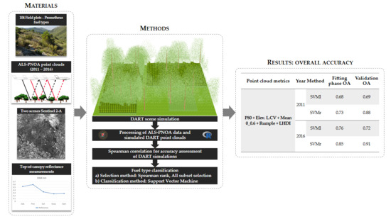
Table 8. Comparison between support vector machine with radial kernel (SVMr) and support vector machine with linear kernel (SVMl) classification method using overall accuracy for the selected metrics based on Spearman correlation. OA stands for overall accuracy.
MetricsYearMethodFitting phase OAValidation OA
P80 + Elev. L.CV + Mean 0_0.6 + Rumple+ LHDI2011SVMl0.680.69
SVMr0.730.88
2016SVMl0.760.72
SVMr0.850.91
Table 9. Overall accuracy of all subsect selection selected metrics using SVMr classification method. seqrep stands for sequential replacement.
YearMetricsApproachFitting PhaseValidation
2011P30+ Elev.CV + Prop. 2.5_3 + Prop. above_4seqrep and Exhaustive0.720.72
P30+ Elev. L.CV+ % first ret. Above meanForward0.750.74
P30+ Elev. L.CV+ Prop 0.5_1+ Mean above_4Backward0.690.74
2016 P95+ P99+ Mean 0_0.6+ Prop. 2_4seqrep0.790.78
P60+ Elev. L4+ Median 0_0.6+ Prop. 2_4Exhaustive0.730.79
Elev. SQRT mean SQ + Elev. CUR mean CUBE + Mean 0_0.6 + Max. above_4Forward0.720.72
Elev. max + Mean 0_0.6 + Mode 0_0.6 + Prop. 2_4Backward0.830.84
Table 10. Confusion matrix for the most accurate classification model after validation for year 2011. * Overall accuracy, 1 Mean user´s accuracy, 2 Mean producer accuracy.
Reference
PredictedFuel Type 1Fuel Type 2Fuel Type 3Fuel Type 4Fuel Type 5Fuel Type 6Fuel Type 7Total PlotsUser´s Accuracy (%)
Fuel type 1114000001573.3
Fuel type 2117100001989.5
Fuel type 3131400001877.8
Fuel type 40008100988.9
Fuel type 50000190019100
Fuel type 600001901090.0
Fuel type 70000001414100
Total plots13241582191410488.5 1
Producer´s accuracy (%)84.670.893.310090.510010091.3 288.5 *
Table 11. Confusion matrix for the most accurate classification model after validation for year 2016. * Overall accuracy, 1 Mean user´s accuracy, 2 Mean producer accuracy.
Reference
PredictedFuel Type 1Fuel Type 2Fuel Type 3Fuel Type 4Fuel Type 5Fuel Type 6Fuel Type 7Total PlotsUser´s Accuracy (%)
Fuel type 191000001090.0
Fuel type 2423100002882.1
Fuel type 30014000014100
Fuel type 400080008100
Fuel type 5000021202391.3
Fuel type 600000606100
Fuel type 7000001141593.3
Total plots13241582191410493.8 1
Producer´s accuracy (%)69.295.893.310010066.710089.3 291.3 *
Publisher’s Note: MDPI stays neutral with regard to jurisdictional claims in published maps and institutional affiliations.

