A Novel Machine Learning Approach to Estimate Grapevine Leaf Nitrogen Concentration Using Aerial Multispectral Imagery

 ,
,  ,
, 
Abstract
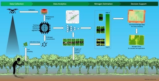
1. Introduction
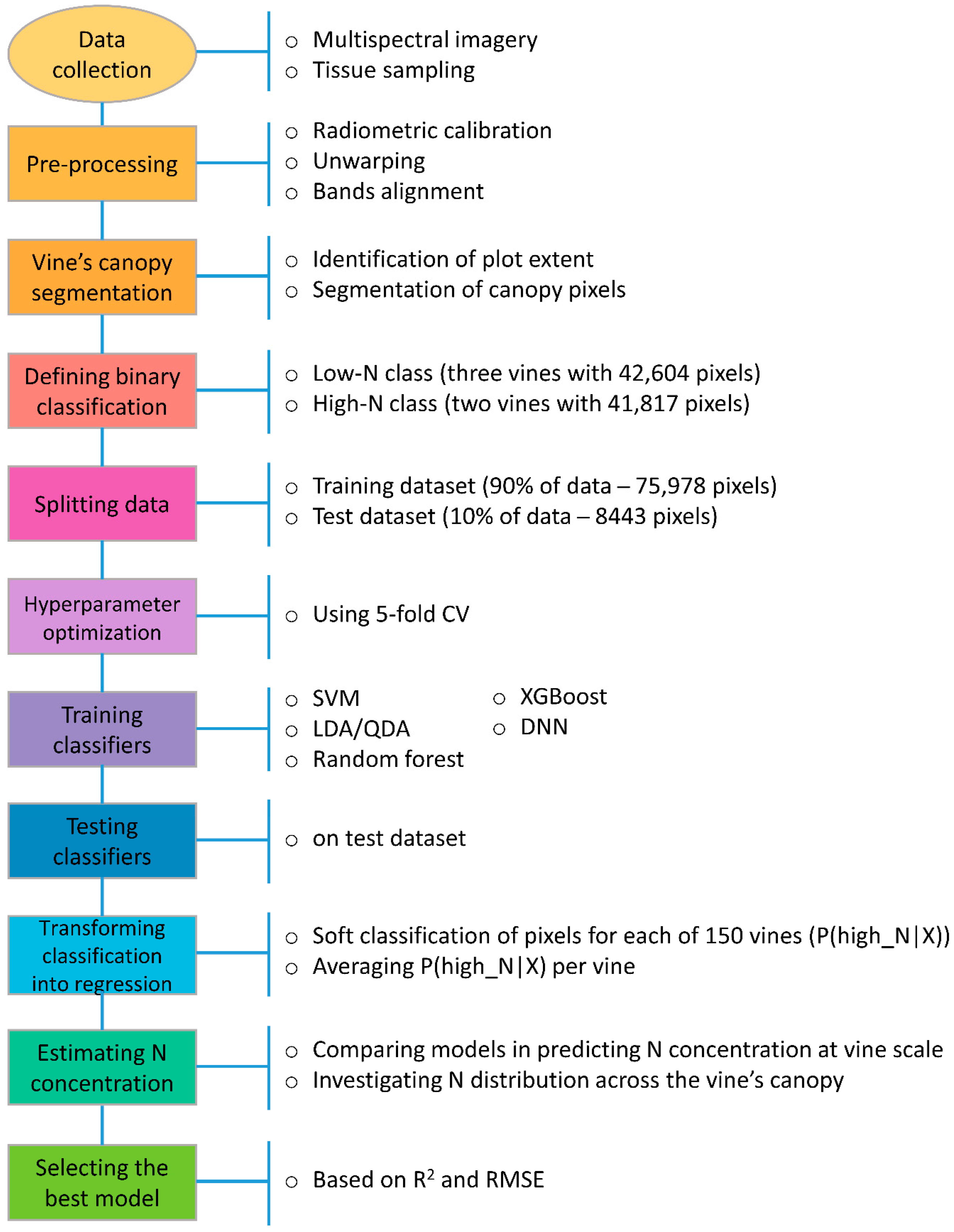
2. Materials and Methods
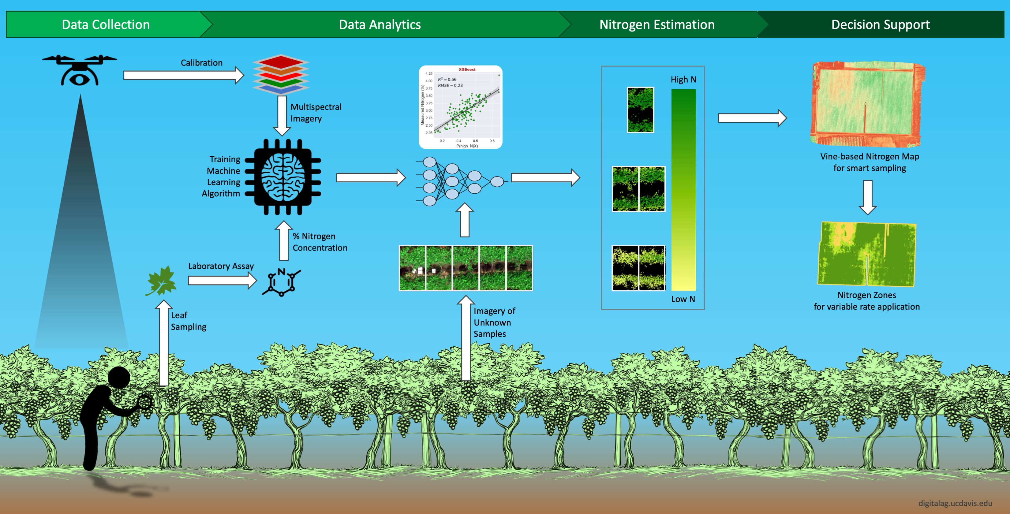
2.1. Experimental Site
2.2. Airborne Multispectral Imaging System
2.3. Aerial Imagery Campaign
2.4. Pre-Processing of Multispectral Images
2.5. Grapevine’s Canopy Segmentation
2.6. Analysis of Multispectral Dataset
2.6.1. Training Machine Learning Classifiers
2.6.2. Hyperparameter Optimization
2.7. Comparing Classifiers on Test Dataset
2.8. Transforming Classification into Regression
3. Results
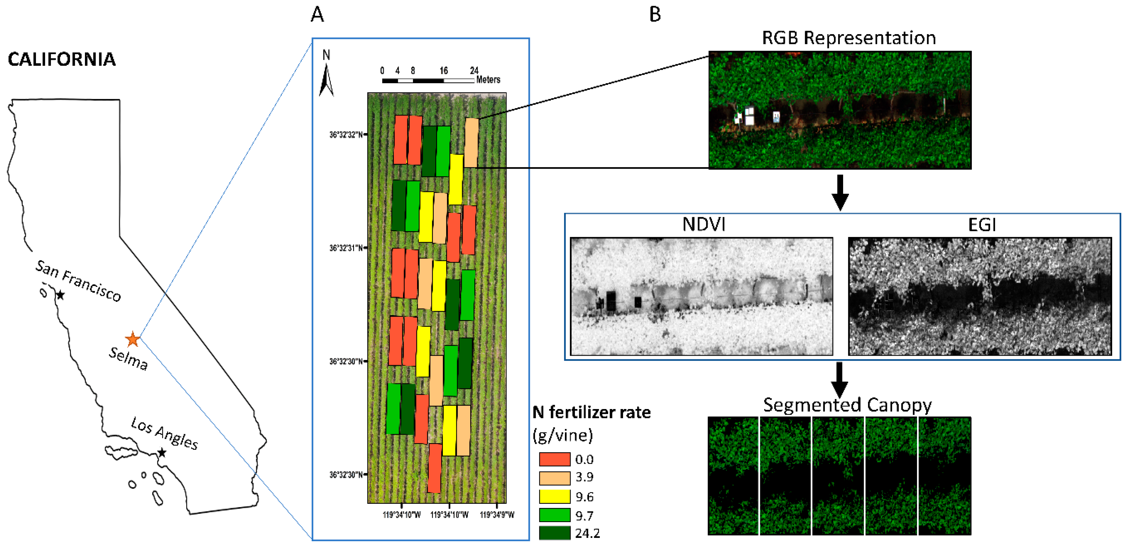
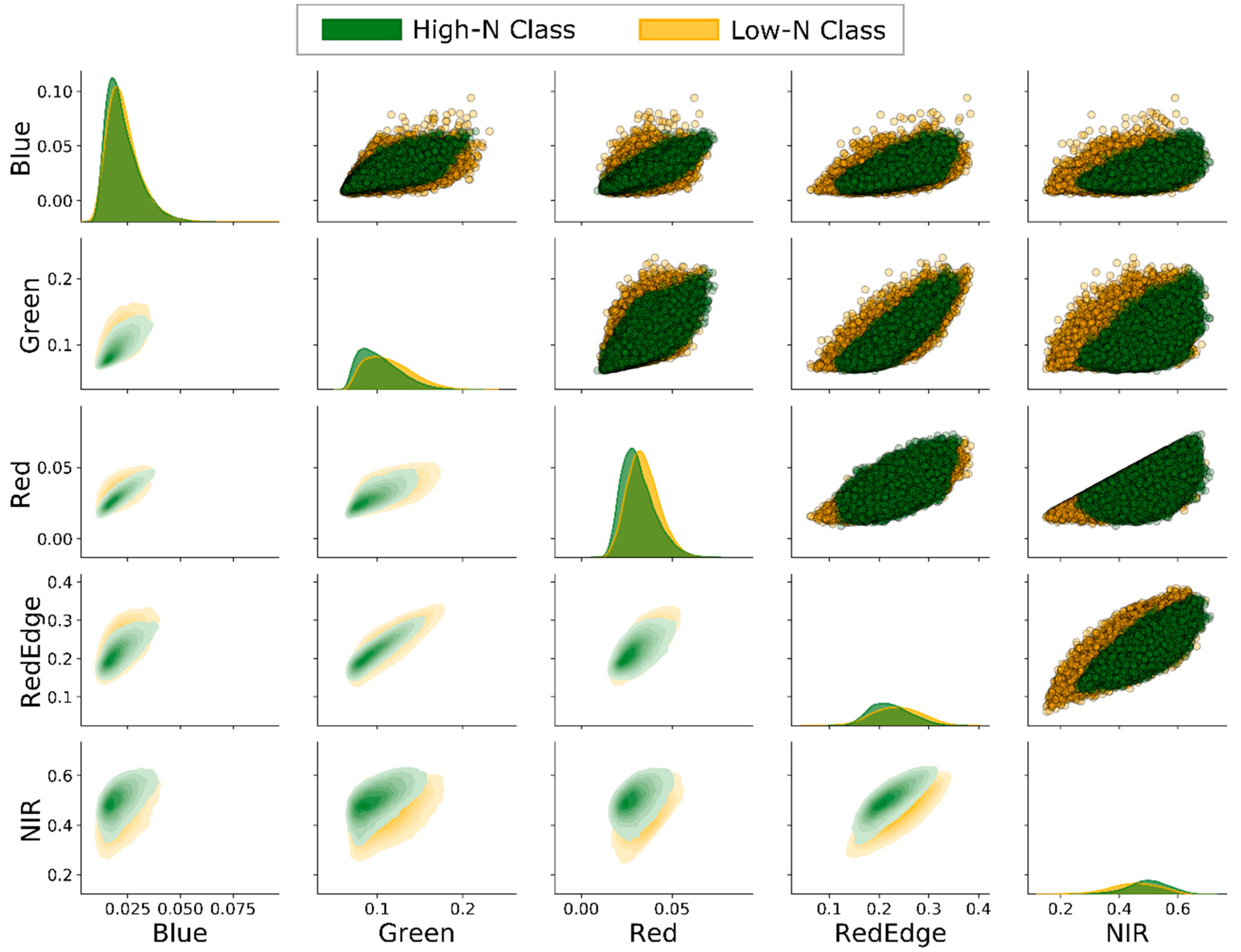
3.1. Bands Pairwise Correlation
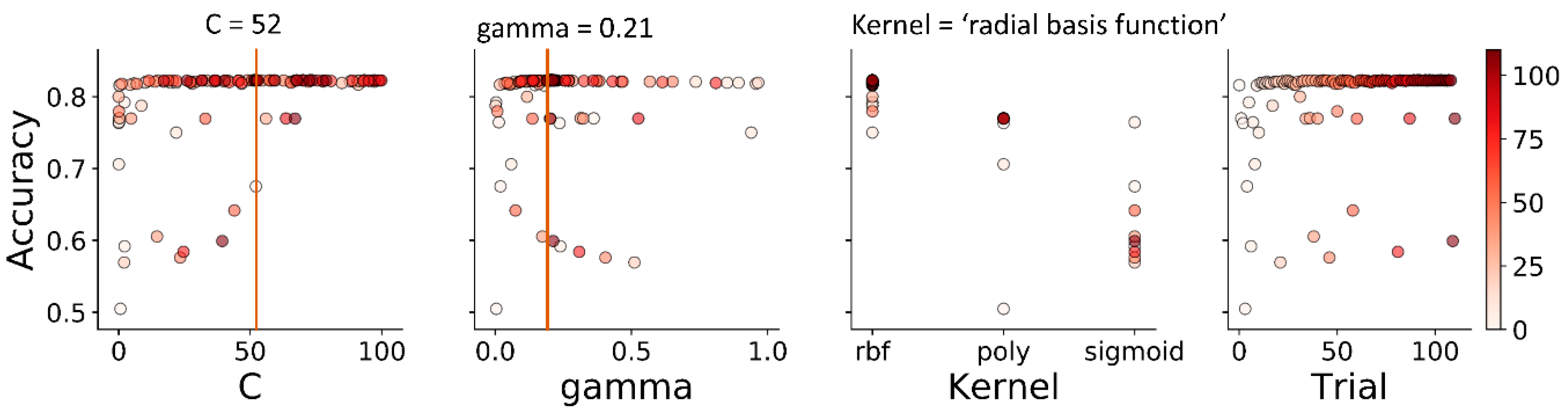
3.2. Hyperparameter Tuning
3.3. Performance of Classifiers
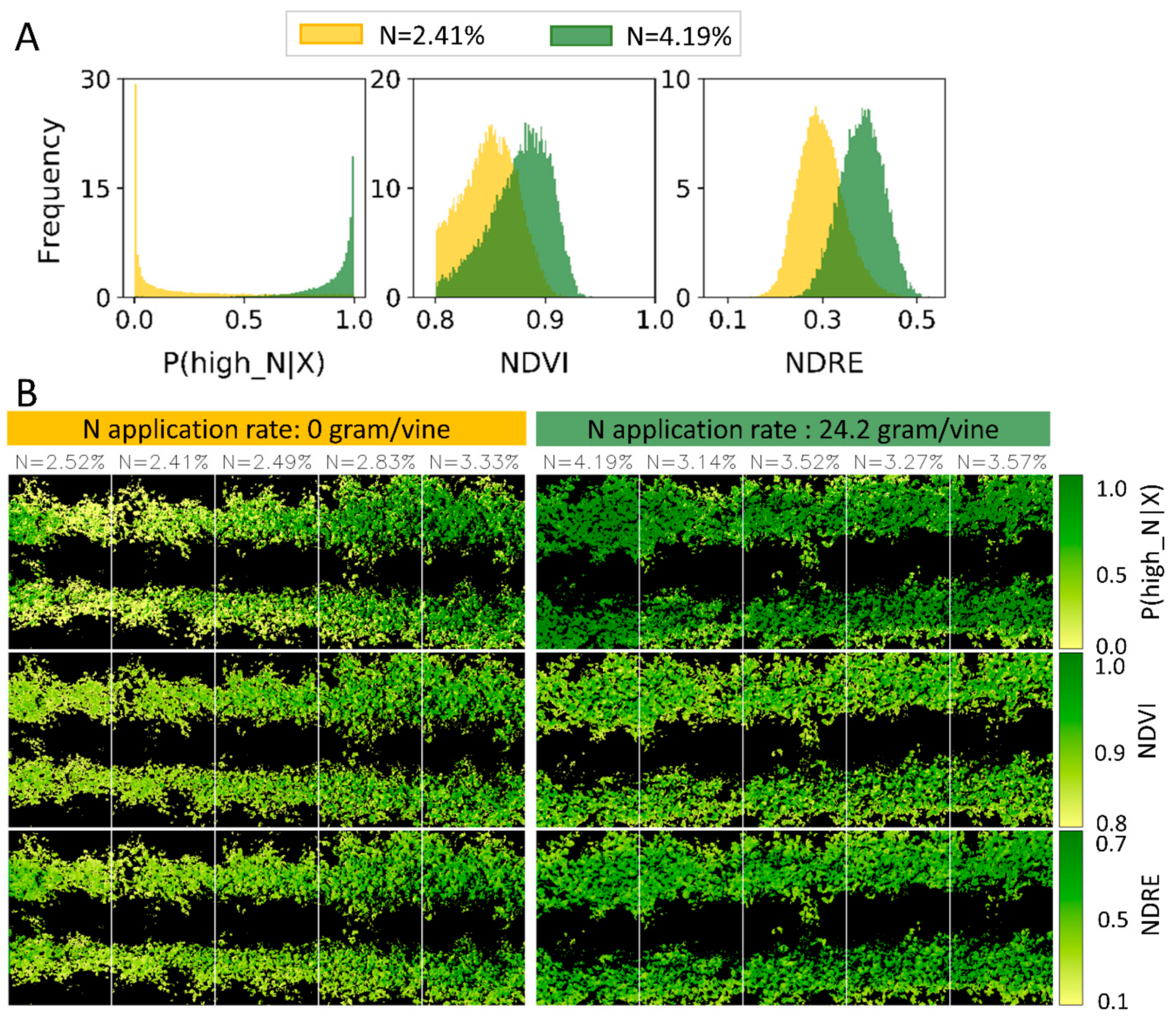
3.4. Nitrogen Prediction of Vines
4. Discussion
4.1. Influence of Leaf Nitrogen Concentration on Spectral Characteristics
4.1.1. Visible Bands (Blue, Green, and Red)
4.1.2. Red Edge Band
4.1.3. Near-Infrared Band
4.2. Significance of the Proposed Data-Driven Method
4.2.1. Appropriate Use of High-Resolution Imagery
4.2.2. Spatial Distribution of N Across the Vine’s Canopy
4.2.3. Adjustable Decision Threshold for Spatial Zoning of Nitrogen
4.2.4. Directed Sampling from Hot Spot in Vineyard
4.3. Limitation of Multispectral Imaging
5. Conclusions
Author Contributions
Funding
Acknowledgments
Conflicts of Interest
Appendix A

| Classifier | Hyperparameters | Search Space Domain | Optimal Parameter |
|---|---|---|---|
| support vector machine (SMV) | “kernel” | (“poly”, ”rbf”, “sigmoid”) | “rbf” |
| “C” | (1 × 10⁻², 1 × 10²) | 52.07 | |
| “gamma” | (1 × 10⁻³, 1 × 100) | 0.21 | |
| discriminant analysis | “classifier” | (QDA, LDA) | QDA |
| “reg_param” (QDA) | (0, 1 × 10⁻³) | 5.27 × 10⁻⁷ | |
| random forest | “n_estimators” | (100, 1000) | 496 |
| “criterion” | (“gini”, “entropy”) | “entropy” | |
| “min_samples_split” | (2, 100) | 38 | |
| “min_samples_leaf” | (2, 50) | 3 | |
| “max_features” | (2, 5) | 2 | |
| “max_depth” | (10, 1000) | 110 | |
| “bootstrap” | (True, False) | TRUE | |
| XGBoost | “num_boost_round” | (100, 1000) | 292 |
| “learning_rate” | (0.01, 0.5) | 0.45 | |
| “feature_fraction” | (0.1, 1.0) | 0.9 | |
| “subsample” | (0.1, 1.0) | 0.94 | |
| “booster” | (“gbtree”, “gblinear”, “dart”) | “gbtree” | |
| “lambda” | (1 × 10⁻⁸, 1.0) | 1.90 × 10⁻⁴ | |
| “alpha” | (1 × 10⁻⁸, 1.0) | 3.60 × 10⁻⁷ | |
| “max_depth” | (1, 9) | 9 | |
| “eta” | (1 × 10⁻⁸, 1.0) | 0.02 | |
| “gamma” | (1 × 10⁻⁸, 1.0) | 3.28 × 10⁻⁵ | |
| “grow_policy” | (“depthwise”, “lossguide”) | “lossguide” | |
| deep neural network (DNN) | “n_hidden_layers” | (1, 10) | 6 |
| “weight_decay” | (1 × 10⁻¹⁰, 1 × 10⁻³) | 4.44 × 10⁻⁸ | |
| “activation” | (“relu”, “sigmoid”, “tanh”) | “tanh” | |
| “n_units_in_hidden_layers” | (4, 10) | (6, 6, 5, 6, 6, 5) | |
| “optimizer” | (“RMSprop”, “Adam”, “SGD”) | “Adam” | |
| “learning_rate” | (1 × 10⁻⁵, 1 × 10⁻¹) | 4.38 × 10⁻³ | |
| “batch_size_power” | (5, 9) | 25 |

References
- Fidelibus, M.W.; Hashim-Buckey, J.; Vasquez, S. Mondo et mercato: Stati Uniti. In L’Uva da Tavola; Angelini, R., Ed.; Bayer CorpScience S.r.l.: Milano, Italy, 2010; pp. 506–518. [Google Scholar]
- Fidelibus, M.; El-kereamy, A.; Zhuang, G.; Haviland, D.; Hembree, K.; Stewart, D. Sample Costs to Establish and Produce Table Grapes. San Joaquin Valley South. Flame Seedless, Early Maturing; UC Agricultural Issues Center: Davis, CA, USA, 2018. [Google Scholar]
- Christensen, L.P.; Peacock, W.L. Mineral nutrition and fertilization. In Raisin Production Manual; Christensen, L.P., Ed.; University of California, Agriculture Natural Resources, Communication Services: Oakland, CA, USA, 2000; pp. 102–114. ISBN 9781879906440. [Google Scholar]
- Anderson, G.; Van Aardt, J.; Bajorski, P.; Heuvel, J.V. Detection of wine grape nutrient levels using visible and near infrared 1nm spectral resolution remote sensing. Auton. Air Ground Sens. Syst. Agric. Optim. Phenotyping 2016, 9866, 98660. [Google Scholar] [CrossRef]
- Christensen, L.P.; Kasimatis, A.N.; Jensen, F.L. Grapevine Nutrition and Fertilization in the San Joaquin Valley; University of California: Berkeley, CA, USA, 1978; ISBN 9780931876257. [Google Scholar]
- Conradie, W.J. Distribution and Translocation of Nitrogen Absorbed During Early Summer by Two-Year-Old Grapevines Grown in Sand Culture. Am. J. Enol. Vitic. 1991, 42, 180–190. [Google Scholar]
- Grechi, I.; Vivin, P.; Hilbert, G.; Milin, S.; Robert, T.; Gaudillère, J.-P. Effect of light and nitrogen supply on internal C: N balance and control of root-to-shoot biomass allocation in grapevine. Environ. Exp. Bot. 2007, 59, 139–149. [Google Scholar] [CrossRef]
- Keller, M.; Kummer, M.; Vasconcelos, C. Soil nitrogen utilisation for growth and gas exchange by grapevines in response to nitrogen supply and rootstock. Aust. J. Grape Wine Res. 2001, 7, 2–11. [Google Scholar] [CrossRef]
- Ferrara, G.; Malerba, A.D.; Matarrese, A.M.S.; Mondelli, D.; Mazzeo, A. Nitrogen Distribution in Annual Growth of ‘Italia’ Table Grape Vines. Front. Plant Sci. 2018, 9, 1374. [Google Scholar] [CrossRef] [PubMed]
- Harter, T.; Lund, J.R.; Darby, J.; Fogg, G.E.; Howitt, R.; Jessoe, K.; Pettygrove, S.G.; Quinn, J.F.; Viers, J.H.; Boyle, D.B.; et al. Addressing Nitrate in California’s Drinking Water with a Focus on Tulare Lake Basin and Salinas Valley Groundwater; Report for the State Water Resources Control Board Report to the Legislature; UC Davis Center for Watershed Sciences: Davis, CA, USA, 2012. [Google Scholar]
- Mills, H.A.; Jones, J.B. Plant Analysis Handbook II; MicroMacro: Athens, GA, USA, 1996; ISBN1 1878148052. ISBN2 9781878148056. [Google Scholar]
- Iland, P.; Dry, P.; Proffitt, T.; Tyerman, S. The Grapevine: From the Science to the Practice of Growing Vines for Wine; Patrick Iland Wine Promotions Pty Ltd.: Adelaide, Australia, 2011; ISBN 9780958160551. [Google Scholar]
- Friedel, M.; Hendgen, M.; Stoll, M.; Löhnertz, O. Performance of reflectance indices and of a handheld device for estimating in-field the nitrogen status of grapevine leaves. Aust. J. Grape Wine Res. 2020, 26, 110–120. [Google Scholar] [CrossRef]
- Ye, X.; Abe, S.; Zhang, S. Estimation and mapping of nitrogen content in apple trees at leaf and canopy levels using hyperspectral imaging. Precis. Agric. 2019, 21, 198–225. [Google Scholar] [CrossRef]
- Min, M.; Lee, W.S. Determination of Significant Wavelengths and Prediction of Nitrogen Content for Citrus. Trans. ASAE 2005, 48, 455–461. [Google Scholar] [CrossRef]
- Zarate-Valdez, J.L.; Muhammad, S.; Saa, S.; Lampinen, B.D.; Brown, P.H. Light interception, leaf nitrogen and yield prediction in almonds: A case study. Eur. J. Agron. 2015, 66, 1–7. [Google Scholar] [CrossRef]
- Moghimi, A.; Yang, C.; Anderson, J.A. Aerial hyperspectral imagery and deep neural networks for high-throughput yield phenotyping in wheat. Comput. Electron. Agric. 2020, 172, 105299. [Google Scholar] [CrossRef]
- Gitelson, A.A. Wide Dynamic Range Vegetation Index for Remote Quantification of Biophysical Characteristics of Vegetation. J. Plant Physiol. 2004, 161, 165–173. [Google Scholar] [CrossRef]
- Gitelson, A.A.; Kaufman, Y.J.; Merzlyak, M.N. Use of a green channel in remote sensing of global vegetation from EOS-MODIS. Remote Sens. Environ. 1996, 58, 289–298. [Google Scholar] [CrossRef]
- Pacheco-Labrador, J.; Gonzalez-Cascon, R.; Martín, M.P.; Riaño, D. Understanding the optical responses of leaf nitrogen in Mediterranean Holm oak (Quercus ilex) using field spectroscopy. Int. J. Appl. Earth Obs. Geoinf. 2014, 26, 105–118. [Google Scholar] [CrossRef]
- Kokaly, R. Spectroscopic Determination of Leaf Biochemistry Using Band-Depth Analysis of Absorption Features and Stepwise Multiple Linear Regression. Remote Sens. Environ. 1999, 67, 267–287. [Google Scholar] [CrossRef]
- Hansen, P.M.; Schjoerring, J.K. Reflectance measurement of canopy biomass and nitrogen status in wheat crops using normalized difference vegetation indices and partial least squares regression. Remote Sens. Environ. 2003, 86, 542–553. [Google Scholar] [CrossRef]
- Tian, Y.; Yao, X.; Yang, J.; Cao, W.; Hannaway, D.; Zhu, Y. Assessing newly developed and published vegetation indices for estimating rice leaf nitrogen concentration with ground- and space-based hyperspectral reflectance. Field Crop. Res. 2011, 120, 299–310. [Google Scholar] [CrossRef]
- Cho, M.A.; Skidmore, A.K. A new technique for extracting the red edge position from hyperspectral data: The linear extrapolation method. Remote Sens. Environ. 2006, 101, 181–193. [Google Scholar] [CrossRef]
- Ferwerda, J.G.; Skidmore, A.K.; Mutanga, O. Nitrogen detection with hyperspectral normalized ratio indices across multiple plant species. Int. J. Remote Sens. 2005, 26, 4083–4095. [Google Scholar] [CrossRef]
- Esgario, J.G.; Krohling, R.A.; Ventura, J.A. Deep learning for classification and severity estimation of coffee leaf biotic stress. Comput. Electron. Agric. 2020, 169, 105162. [Google Scholar] [CrossRef]
- Qiu, R.; Yang, C.; Moghimi, A.; Zhang, M.; Steffenson, B.J.; Hirsch, C.D. Detection of Fusarium Head Blight in Wheat Using a Deep Neural Network and Color Imaging. Remote Sens. 2019, 11, 2658. [Google Scholar] [CrossRef]
- Tong, H.; Madison, I.; Long, T.; Williams, C.M. Computational solutions for modeling and controlling plant response to abiotic stresses: A review with focus on iron deficiency. Curr. Opin. Plant Biol. 2020, 57, 8–15. [Google Scholar] [CrossRef]
- Moghimi, A.; Yang, C.; Miller, M.E.; Kianian, S.F.; Marchetto, P.M. A Novel Approach to Assess Salt Stress Tolerance in Wheat Using Hyperspectral Imaging. Front. Plant Sci. 2018, 9, 1182. [Google Scholar] [CrossRef]
- Berger, K.; Verrelst, J.; Féret, J.-B.; Hank, T.; Wocher, M.; Mauser, W.; Camps-Valls, G. Retrieval of aboveground crop nitrogen content with a hybrid machine learning method. Int. J. Appl. Earth Obs. Geoinf. 2020, 92, 102174. [Google Scholar] [CrossRef]
- Nigon, T.J.; Yang, C.; Paiao, G.D.; Mulla, D.J.; Knight, J.F.; Fernández, F.G. Prediction of Early Season Nitrogen Uptake in Maize Using High-Resolution Aerial Hyperspectral Imagery. Remote Sens. 2020, 12, 1234. [Google Scholar] [CrossRef]
- Moghimi, A.; Yang, C.; Marchetto, P.M. Ensemble Feature Selection for Plant Phenotyping: A Journey from Hyperspectral to Multispectral Imaging. IEEE Access 2018, 6, 56870–56884. [Google Scholar] [CrossRef]
- Espejo-Garcia, B.; Mylonas, N.; Athanasakos, L.; Fountas, S.; Vasilakoglou, I. Towards weeds identification assistance through transfer learning. Comput. Electron. Agric. 2020, 171, 105306. [Google Scholar] [CrossRef]
- Pantazi, X.; Tamouridou, A.; Alexandridis, T.K.; Lagopodi, A.; Kashefi, J.; Moshou, D. Evaluation of hierarchical self-organising maps for weed mapping using UAS multispectral imagery. Comput. Electron. Agric. 2017, 139, 224–230. [Google Scholar] [CrossRef]
- Feng, L.; Zhang, Z.; Ma, Y.; Du, Q.; Williams, P.; Drewry, J.; Luck, B. Alfalfa Yield Prediction Using UAV-Based Hyperspectral Imagery and Ensemble Learning. Remote Sens. 2020, 12, 2028. [Google Scholar] [CrossRef]
- Gavlak, R.; Horneck, D.; Miller, R.O. Soil, Plant and Water Reference Methods for the Western Region 1, 3rd ed.; Western Rural Development Center (WREP-125): Logan, UT, USA, 2005. [Google Scholar]
- Moghimi, A. Micasense_Preprocessing (Version 1.0.0). 2020. Available online: https://doi.org/10.5281/zenodo.3988680 (accessed on 20 June 2020).
- Pedregosa, F.; Varoquaux, G.; Gramfort, A.; Michel, V.; Thirion, B.; Grisel, O.; Blondel, M.; Prettenhofer, P.; Weiss, R.; Dubourg, V.; et al. Scikit-learn: Machine Learning in Python. J. Mach. Learn. Res. 2011, 12, 2825–2830. [Google Scholar]
- Chen, T.; Guestrin, C. XGBoost: A Scalable Tree Boosting System. In Proceedings of the 22nd ACM SIGKDD International Conference on Knowledge Discovery and Data Mining, San Francisco, CA, USA, 13–17 August 2016; ACM: New York, NY, USA, 2016; pp. 785–794. [Google Scholar]
- Abadi, M.; Agarwal, A.; Paul Barham, E.B.; Chen, Z.; Citro, C.; Corrado, G.S.; Davis, A.; Dean, J.; Devin, M.; Ghemawat, S.; et al. TensorFlow: Large-scale machine learning on heterogeneous systems. arXiv 2015, arXiv:1603.04467. [Google Scholar]
- Li, L.; Jamieson, K.; Rostamizadeh, A.; Gonina, E.; Ben-tzur, J.; Hardt, M.; Recht, B.; Talwalkar, A. A System for Massively Parallel Hyperparameter Tuning. In Proceedings of the Machine Learning and Systems, Austin, TX, USA, 2–4 March 2020; pp. 230–246. [Google Scholar]
- Bergstra, J.; Bengio, Y. Random Search for Hyper-Parameter Optimization. J. Mach. Learn. Res. 2012, 13, 281–305. [Google Scholar]
- Bergstra, J.; Bardenet, R.; Bengio, Y.; Kégl, B. Algorithms for Hyper-Parameter Optimization. In Advances in Neural Information Processing Systems 24; Shawe-Taylor, J., Zemel, R.S., Bartlett, P.L., Pereira, F., Weinberger, K.Q., Eds.; Curran Associates, Inc.: New York, NY, USA, 2011; pp. 2546–2554. [Google Scholar]
- Snoek, J.; Larochelle, H.; Adams, R.P. Practical Bayesian Optimization of Machine Learning Algorithms. In Proceedings of the 25th International Conference on Neural Information Processing Systems—Volume 2; Curran Associates Inc.: Red Hook, NY, USA, 2012; pp. 2951–2959. [Google Scholar]
- Bergstra, J.; Yamins, D.; Cox, D.D. Making a Science of Model Search: Hyperparameter Optimization in Hundreds of Dimensions for Vision Architectures. In Proceedings of the 30th International Conference on Machine Learning, Atlanta, GA, USA, 16–21 June 2013; Volume 28. [Google Scholar]
- Franceschi, L.; Donini, M.; Frasconi, P.; Pontil, M. Forward and Reverse Gradient-Based Hyperparameter Optimization. In Proceedings of the 34th International Conference on Machine Learning, Sydney, Australia, 6–11 August 2017. [Google Scholar]
- Akiba, T.; Sano, S.; Yanase, T.; Ohta, T.; Koyama, M. Optuna: A Next-generation Hyperparameter Optimization Framework. In Proceedings of the 25rd ACM SIGKDD International Conference on Knowledge Discovery and Data Mining, Anchorage, AK, USA, 25 July 2019. [Google Scholar]
- Tan, P.-N.; Steinbach, M.; Kumar, V. Introduction to Data Mining, 1st ed.; Addison-Wesley Longman Publishing Co., Inc.: Boston, MA, USA, 2005; ISBN 0321321367. [Google Scholar]
- Platt, J.C.; Platt, J.C. Probabilistic Outputs for Support Vector Machines and Comparisons to Regularized Likelihood Methods. Adv. Large Margin Classif. 1999, 10, 61–74. [Google Scholar]
- Peñuelas, J.; Filella, I. Visible and near-infrared reflectance techniques for diagnosing plant physiological status. Trends Plant Sci. 1998, 3, 151–156. [Google Scholar] [CrossRef]
- Peñuelas, J.; Gamon, J.; Fredeen, A.; Merino, J.; Field, C. Reflectance indices associated with physiological changes in nitrogen- and water-limited sunflower leaves. Remote Sens. Environ. 1994, 48, 135–146. [Google Scholar] [CrossRef]
- Daughtry, C. Estimating Corn Leaf Chlorophyll Concentration from Leaf and Canopy Reflectance. Remote Sens. Environ. 2000, 74, 229–239. [Google Scholar] [CrossRef]
- Zhao, D.; Reddy, K.R.; Kakani, V.G.; Reddy, V. Nitrogen deficiency effects on plant growth, leaf photosynthesis, and hyperspectral reflectance properties of sorghum. Eur. J. Agron. 2005, 22, 391–403. [Google Scholar] [CrossRef]
- Ayala-Silva, T.; Beyl, C.A. Changes in spectral reflectance of wheat leaves in response to specific macronutrient deficiency. Adv. Space Res. 2005, 35, 305–317. [Google Scholar] [CrossRef]
- Filella, I.; Penuelas, J. The red edge position and shape as indicators of plant chlorophyll content, biomass and hydric status. Int. J. Remote Sens. 1994, 15, 1459–1470. [Google Scholar] [CrossRef]
- Gates, D.M.; Keegan, H.J.; Schleter, J.C.; Weidner, V.R. Spectral Properties of Plants. Appl. Opt. 1965, 4, 11–20. [Google Scholar] [CrossRef]
- Knipling, E.B. Physical and physiological basis for the reflectance of visible and near-infrared radiation from vegetation. Remote Sens. Environ. 1970, 1, 155–159. [Google Scholar] [CrossRef]
- Slaton, M.R.; Hunt, E.R.; Smith, W.K. Estimating near-infrared leaf reflectance from leaf structural characteristics. Am. J. Bot. 2001, 88, 278–284. [Google Scholar] [CrossRef]
- Hikosaka, K.; Anten, N.P.R.; Borjigidai, A.; Kamiyama, C.; Sakai, H.; Hasegawa, T.; Oikawa, S.; Iio, A.; Watanabe, M.; Koike, T.; et al. A meta-analysis of leaf nitrogen distribution within plant canopies. Ann. Bot. 2016, 118, 239–247. [Google Scholar] [CrossRef] [PubMed]
- Poni, S.; Intrieri, C.; Silvestroni, O. Interactions of LeafAge, Fruiting, and Exogenous Cytokinins in Sangiovese Grapevines under Non-Irrigated Conditions. II. Chlorophyll and Nitrogen Content. Am. J. Enol. Vitic. 1994, 45, 278–284. [Google Scholar]
- Huang, C.H.; Singh, G.P.; Park, S.H.; Chua, N.-H.; Ram, R.J.; Park, B.S. Early Diagnosis and Management of Nitrogen Deficiency in Plants Utilizing Raman Spectroscopy. Front. Plant Sci. 2020, 11, 663. [Google Scholar] [CrossRef]
- Zarco-Tejada, P.J.; González-Dugo, V.; Williams, L.E.; Suárez, L.; Berni, J.A.J.; Goldhamer, D.A.; Fereres, E. A PRI-based water stress index combining structural and chlorophyll effects: Assessment using diurnal narrow-band airborne imagery and the CWSI thermal index. Remote Sens. Environ. 2013, 138, 38–50. [Google Scholar] [CrossRef]
- Omidi, R.; Moghimi, A.; Pourreza, A.; Aly, M.E.-H.; Eddin, A.S. Ensemble Hyperspectral Band Selection for Detecting Nitrogen Status in Grape Leaves. arXiv 2020, arXiv:2010.04225. [Google Scholar]


| Bands | Center Wavelength (nm) | Bandwidth FWHM * |
|---|---|---|
| Blue | 475 | 20 |
| Green | 560 | 20 |
| Red | 668 | 10 |
| Red Edge | 717 | 10 |
| Near-infrared | 840 | 40 |
| Classifier | Test Dataset | Training Dataset | |||||||
|---|---|---|---|---|---|---|---|---|---|
| F1 1 (%) | Precision (%) | Recall (%) | AUC 2 (%) | Threshold 3 | Training time (s) | Prediction time (s) | F1 –mean (%) | F1 StD 4 | |
| SVM | 82.24 | 82.35 | 82.25 | _ | _ | 128.59 | 3.45 | 82.25 | 0.32 |
| QDA | 80.85 | 80.96 | 80.86 | 89.01 | 0.54 | 0.02 | 0.01 | 80.40 | 0.30 |
| Random Forest | 81.81 | 81.81 | 81.81 | 90.25 | 0.51 | 91.39 | 0.62 | 81.55 | 0.23 |
| XGBoost | 80.27 | 80.29 | 80.27 | 88.29 | 0.51 | 7.29 | 0.02 | 80.94 | 0.31 |
| DNN | 81.68 | 81.79 | 81.69 | 89.90 | 0.52 | 316.09 | 0.57 | 81.34 | 0.52 |
| Ensemble | 82.24 | 82.31 | 82.25 | 90.31 | _ | 543.37 | 4.66 | _ | _ |
Publisher’s Note: MDPI stays neutral with regard to jurisdictional claims in published maps and institutional affiliations. |
© 2020 by the authors. Licensee MDPI, Basel, Switzerland. This article is an open access article distributed under the terms and conditions of the Creative Commons Attribution (CC BY) license (http://creativecommons.org/licenses/by/4.0/).
Share and Cite
Moghimi, A.; Pourreza, A.; Zuniga-Ramirez, G.; Williams, L.E.; Fidelibus, M.W. A Novel Machine Learning Approach to Estimate Grapevine Leaf Nitrogen Concentration Using Aerial Multispectral Imagery. Remote Sens. 2020, 12, 3515. https://doi.org/10.3390/rs12213515
Moghimi A, Pourreza A, Zuniga-Ramirez G, Williams LE, Fidelibus MW. A Novel Machine Learning Approach to Estimate Grapevine Leaf Nitrogen Concentration Using Aerial Multispectral Imagery. Remote Sensing. 2020; 12(21):3515. https://doi.org/10.3390/rs12213515
Chicago/Turabian StyleMoghimi, Ali, Alireza Pourreza, German Zuniga-Ramirez, Larry E. Williams, and Matthew W. Fidelibus. 2020. "A Novel Machine Learning Approach to Estimate Grapevine Leaf Nitrogen Concentration Using Aerial Multispectral Imagery" Remote Sensing 12, no. 21: 3515. https://doi.org/10.3390/rs12213515
APA StyleMoghimi, A., Pourreza, A., Zuniga-Ramirez, G., Williams, L. E., & Fidelibus, M. W. (2020). A Novel Machine Learning Approach to Estimate Grapevine Leaf Nitrogen Concentration Using Aerial Multispectral Imagery. Remote Sensing, 12(21), 3515. https://doi.org/10.3390/rs12213515