1. Introduction
Vision-based control of underwater vehicles enables autonomous operations. It facilitates complex missions, including surveillance of pipelines [
1], inspection of cables [
2], docking of vehicles [
3], deep-sea exploration [
4], and ship hull inspection [
5]. These tasks require continuous visual feedback obtained from either monocular or stereo vision systems [
6]. In order to improve performance, the vision system is often supported by acoustic and inertial sensors [
7].
Therefore, a more practical approach is the use of multi-sensors in Autonomous Underwater Vehicles (AUVs) as they perform missions with full autonomy. Consequently, long-term operations in unknown environments are achievable. The most common collaborating devices for this purpose are [
8]: the Doppler Velocity Log (DVL); the Inertial Navigation System (INS); the Inertial Measurement Unit (IMU); and the Sound Navigation And Ranging (SONAR). They also include: the Acoustic Aided Navigation inclusive of the Long Base Line (LBL), the Short Base Line (SBL), and the Ultra Short Base Line (USBL). Ultimately, each vehicle is equipped with a compass and a pressure sensor. These devices can support RGB cameras, especially during a distance operation to a bottom where a clear optical inspection is taxing.
The multi-sensors approach allows the configuration of a measurement system that is composed of several devices. Therefore, to analyse the different sensors’ configurations, research has been conducted in this field. Some of this research has classified the current sensors’ fusion techniques for unmanned underwater vehicle navigation [
9]. The authors of this classification primarily focused on the fusion architecture in terms of the vehicle’s tasks. Moreover, underwater vehicle localisation in shallow water was addressed in [
10], which utilised an Attitude Heading Reference System (AHRS), a pressure sensor, a GPS, a USBL, and a DVL. According to the authors, it was reliable even with some of the sensors temporarily switched off. Furthermore, based on raw measurements from the SBL, the Inverted Ultrashort Baseline (iUSBL), the IMU, and a pressure sensor and the SBL, a further solution was presented in [
11]. This solution proved its benefit in mining applications, allowing an operator to control the mining vehicle utilising virtual reality depiction. A final addition is the sensor fusion of an acoustic positioning system, the DVL, the IMU and a pressure gauge that was presented in [
12]. The authors of this research proposed a hybrid translational observer concept for underwater navigation.
Despite various sensors and measurement systems being used to navigate underwater vehicles, only a few of them are employed in inspection-class vehicles. This is because this vehicle type, equipped with propellers and a camera, is mainly devoted to gathering pictures from the underwater scene. Additionally, it is furnished with low-cost sensors, such as a pressure gauge, a compass, and an IMU [
13]. This equipment is efficient for remote control, supervised by a human operator. Thus, inspection-class vehicles are seldom equipped with DVL, INS, and SONAR systems due to their high cost, which increases as the required quality of measurement is raised. Moreover, acoustic-aided navigation systems are only used during operations on a larger area due to a measurement precision of a few metres. Alternating this for small areas, cameras, echo sounders, and laser rangefinders are considered for the control of inspection-class vehicles.
RGB cameras are a viable option in AUVs for the operations of both Visual Odometry (VO) and Visual Simultaneous Localization and Mapping (VSLAM), which facilitate the vehicle’s navigation in large areas [
4,
14,
15,
16,
17,
18]. VO is a process of estimating a change in position over time using sequential camera images. VSLAM is also a process that, in addition to position estimation, creates an environmental map and localises a vehicle within the map simultaneously. The latter process has been at the centre of recent research. For example, Cui et al. [
19] proposed a pose estimation method based on the Projective Vector with noise error uncertainty. The results discussed in the research reported that the pose estimation method has robustness and convergence while managing different degrees of error uncertainty. Further research in [
20] improved variance reduction in fast simultaneous localisation and mapping (FastSLAM). FastSLAM introduced simulated annealing to resolve the issues of particle degradation, depletion, and loss, which lead to a reduction in the AUV location estimation accuracy.
A distortion caused by the deep water’s visual degradation impedes both processes. This is because strong light absorption reduces visual perception up to a few metres, while backscattered light propagation has effects on the acquired images [
21]. To overcome these impediments, some researchers select sonar systems to manage underwater navigation, which serves the purpose of eliminating the visual-degradation effect [
22]. However, resorting to this leads to obtaining data that have the quality of reduced spatial and temporal resolution. Therefore, RGB cameras are the optimum solution for AUV operations that are at a close distance from the bottom.
Our previous research [
23,
24] indicates that usage of RGB cameras during underwater missions in the Baltic Sea, as well as in the Polish lakes, is very limited. This is due to the low visibility that allows operating at only a few metres from the bottom. Consequently, the position of the vehicle can be estimated primarily using the DVL and INS systems. Even though the implementation of RGB cameras for the AUVs in terms of underwater navigation is impracticable in our region, there is still the space to utilise them for underwater exploration carried out using Remotely Operated Vehicles (ROVs). They can be implemented in applications such as intervention, repair and maintenance in offshore industries, and naval defence and for scientific purposes [
25,
26,
27]. Other employments involve the autonomous docking of the vehicle [
3,
28] and cooperation with a diver [
29].
Some missions necessitate the gathering of pictures from the underwater scene in preparation for subsequent analysis. For example, any crime scene is video recorded and based on the presented video footage; the prosecutor can use it for investigation purposes [
30]. In that case, the vehicle’s movement is required to be both on a set track with low speed and at a calculated distance from the bottom. Thus, by applying these requirements, the ROV is ready to gather representative footage. Cameras, echo sounders, and laser rangefinders are present to facilitate the automatic operations. The cameras enable calculation of both the speed and the distance from the bottom, while echo sounders and laser rangefinders compute the measurement of the distance from the bottom. The functions of these sensors also apply to the SLAM technique. However, it is not considered the best option for the precision of the vehicle’s movement in a small area. So, with the target of a more precise vehicle motion, visual servo control was designated for various robotic applications [
31]. It facilitates precise control because it calculates error values in the close-loop control, using feedback information extracted from a vision sensor. Therefore, we decided to employ this technique in the method under consideration. Additionally, we refrained from using an echo sounder, due to its high price, or a laser rangefinder, because it measures the distance to one point on the bottom. This limitation precludes the development of a complex algorithm in the case of the presence of obstacles at the bottom.
In terms of underwater operations, visual servoing has been mainly utilised in AUVs [
1,
6,
32,
33]. Some researchers have also used this technique in ROVs for vehicle docking [
3,
32], vehicle navigation [
34], work-class vehicle control [
35], and manipulator control [
33]. Nevertheless, to the knowledge of the authors, previous research has not been as devoted as this one to utilising visual servoing for precise vehicle control at low speed and a calculated distance from the bottom in a small area.
However, control of the ROV for the determined distance from the bottom using one camera is problematic because the distance to the object cannot be estimated in this case. To tackle this problem, some researchers have used laser pointers or lines [
36,
37] for distance measurement. Conversely, recent development in optical sensors, as well as the capability of modern computers, allows the capturing and real-time processing of images from more than one camera. For this purpose, the most popular solution is a stereo vision system, which comprises two cameras, mostly parallel and located near each other. This solution enables distance measurement utilising the parallax phenomenon. It also facilitates depth perception based on disparity calculation.
To further explain, stereo vision systems are especially suitable for ROVs, for which the higher-order computation tasks can be performed by a computer located on the surface. The high computational cost, in the case of visual servo control of underwater vehicles, derives from the fact that images should be simultaneously analysed, not only in stereo-pair depiction but also in consecutive frames. For AUVs, where all the calculations are executed on board, the complex image-processing algorithms demand more computing and energy resources. Such demands can result in the need for a bigger size for the vehicle, which in turn means a higher cost for manufacturing. Finally, the stereo vision systems implemented on AUVs are mostly devoted to distance measurement and post-processing depth perception.
The stereo vision system has been used in various underwater applications. For example, an ROV’s position estimation was presented in [
38]. Rizzini et al. [
39] also demonstrated the stereo vision system’s ability for pipeline detection. In their research, the authors proposed the integration of a stereo vision system in the MARIS intervention AUV for detecting cylindrical pipes. Birk et al. [
40] complemented previous research by introducing a solution that reduces the robot operators’ offshore workload through a recommended onshore control centre that runs operations. In their method, the user interacts with a real-time simulation environment; then, a cognitive engine analyses the user’s control requests. Subsequently, with the requests turned into movement primitives, the ROV autonomously executes these primitives in the real environment.
Reference [
41] presented a stereo vision system for deep-sea operations. The system comprises cameras in pressure bottles that are daisy-chained to a computer bottle. The system has substantial computation power for on-board stereo processing as well as for further computer vision methods to support autonomous intelligent functions, e.g., object recognition, navigation, mapping, inspection, and intervention. Furthermore [
42], by means of the stereo vision system, presented an application that detects underwater objects. However, experimental results revealed that the application’s range for detecting simple objects in an underwater environment is limited. Another application is ship hull inspection, which was introduced in [
43]. The stereo vision system was made part of the underwater vehicle systems to estimate normal surface vectors. The system also allows the vehicle to navigate the hull in flat and over moderately curved surface areas. It is important to note that a stereo-vision hardware setup and the software, developed using the ROS middleware, were presented in [
44], where the authors devoted their solution to cylindrical pipe detection.
Overall, even though vision systems have been implemented in some underwater applications, very few of them have been devoted to controlling underwater vehicles. This is mainly attributable to the high computational cost, which restricts real-time operations. However, as the performance of modern cameras and computers allows for the real-time processing of multiple images, we decided to utilise a stereo vision system for the vision-based control of inspection-class ROVs. To this aim, we developed an application based on the image-feature tracking technique. As feature detection constitutes a challenging task in the underwater environment, the first step in our work was to perform analyses based on images and videos from prospective regions of the vehicles’ missions. This approach allowed us to evaluate the control system of the vehicle in a swimming pool, which would be very challenging in the real environment.
The primary assumption for the devised method is that the one loop of the algorithm performs quickly enough to effectively control the vehicle in the case of precise movement at a low speed. Thus, all the algorithms developed for the method, such as image enhancement, image-feature detection and tracking, or stereo correspondence determination, were developed to meet this requirement. In our solution, we utilised a compass and an IMU to facilitate the heading control as well as simplify the speed-control algorithms. Even though the devised system measures heading, its calculation is highly subject to the bias which stems from the integration error, which arises during the time of operation. Additionally, a compass is needed to decide the initially measured heading. Therefore, we resolved to employ a compass in the measurement system because of its low cost and higher precision. Furthermore, a pressure sensor was used to verify the distance from the bottom during trials in a swimming pool. Simultaneously, the vehicle’s speed and heading were calculated using a vision system presented in [
45]. Our results, obtained using the VideoRay Pro 4 vehicle, indicate that the proposed solution facilitates the precise control of inspection-class ROVs.
In order to adopt our proposed solution, a laptop, two underwater cameras, and a vehicle equipped with compass and depth sensors were used as there was no need for any extra equipment. In our experiments, apart from the VideoRay Pro 4, we utilised two Colour Submergible W/Effio-E DSP Cameras with a Sony Exview Had Ultra High Sensitivity image sensor and a computer with Intel Core i7-6700HQ CPU 2.6 GHz and 32 GB RAM. The computer constitutes a standard laptop.
The remainder of this paper is organised as follows. The details of the proposed method are presented in
Section 2.
Section 3 discusses the experiments conducted to evaluate the practical utility of this approach. Finally, the conclusions are included in
Section 4.
2. Methodology
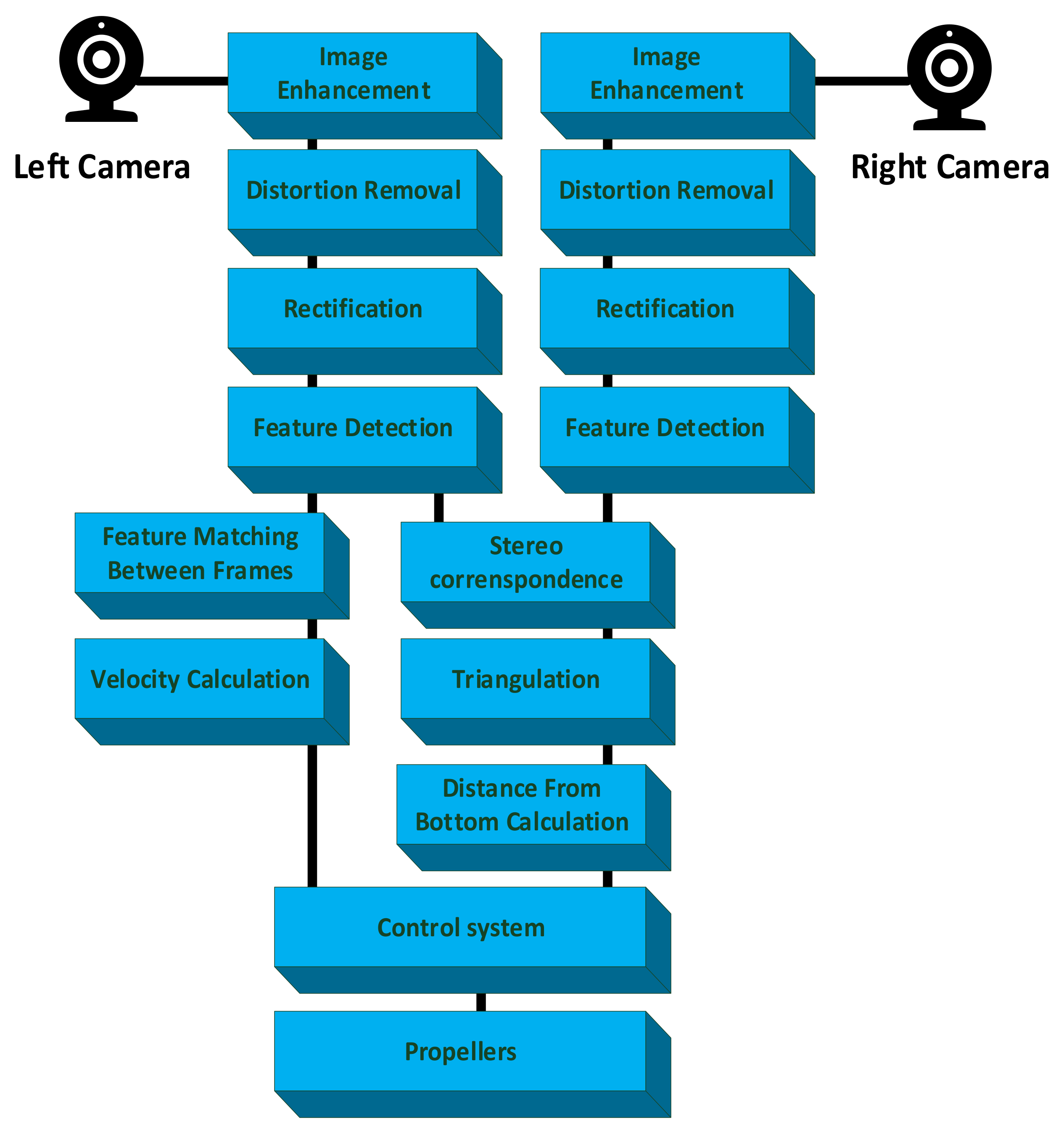
The main goal of this method was to facilitate the vision-based control of inspection-class ROVs. Consequently, local image features were detected and tracked between consecutive images. In this process, time is of the essence because a control signal should be sent to the vehicle at a constant rate. Based on experiments conducted previously, we decided that the intervals should be less than 200 milliseconds [
46]. This time was estimated taking into consideration the vehicle’s dynamic, propeller thrusts, and assumed speed. The obtained results indicated that for a low speed of inspection-class ROVs, a 200-millisecond period was sufficient for all the tested vehicles. As a result, the one loop of the algorithm, comprising feature detection and matching as well as distance calculation and control-signal formation, should be executed in less than 200 milliseconds. This assumption needed the use of the most efficient technique that accomplished the required timeframe. A block diagram depicting the developed method is presented in
Figure 1.
2.1. Underwater Imaging
Underwater imaging poses a difficult task as many variables influence the level of light penetration. For example, the clarity of the water, turbidity, depth, and surface conditions are all variables that affect that level of penetration. Additionally, the depth-rated lens used in deep-sea explorations to provide resistance to high pressure usually leads to nonlinear image distortions. The refraction of light at the water/glass and glass/air connections also results in image deformation. Therefore, as these problems present obstacles, a method based on the mathematical modelling of the underwater environment and another one related to image enhancement have been developed [
47,
48,
49,
50].
As for the mathematical modelling of the underwater environment, it involves the determination of the model’s parameters, including the attenuation coefficient, the object radiance, the scattering coefficient, and, finally, the water transmittance. These parameters are variable and change their value depending on the temperate, depth, salinity, the region of operation, or even the type of marine vegetation. Accordingly, the estimation of these required parameters precedes each ROV’s mission, which makes it time-consuming. As this method is relatively complicated, its implementation in crucial situations is impractical.
The image-enhancement technique, however, is based on digital-image processing. It is devoted to improving the human analysis of underwater, visually distorted scenes. Said analysis takes place in the post-processing phase, which removes the quick execution needed for real-time implementations. Therefore, to develop a solution dedicated to real-time applications, we focused on fast and efficient image-processing techniques, taking into consideration not the human perception, but the number of detected image-feature points. The results of our analysis are presented in
Section 2.2.
Image processing allows an increase in the number of detected image-feature points, but the problem of image distortions remains unsolved. To undistort images, the intrinsic parameters of the camera must be estimated. They can be calculated through the camera calibration process, which constitutes a convenient solution due to plenty of algorithms available in the literature [
51] Some of them have been implemented in computer vision libraries, such as OpenCV or MATLAB Computer Vision System Toolbox [
52]. In our work, the method based on the Zhang and Brown algorithms and applied in the OpenCV library was used. The detailed description of its utilisation is presented in
Section 2.3.
2.2. Local Image Features
Local image features are crucial in many computer vision applications. As opposed to global ones, such as contours, shapes, or textures, they are suitable for determining unique image points, widely utilised in object recognition and tracking. Among the most popular ones, the following can be encountered: SIFT [
53], SURF [
54], BRISK [
55], ORB [
56], HARRIS [
57], FAST [
58], STAR [
59], BRIEF [
60], and FREAK [
61]. The algorithms mentioned above are used to determine the position of distinctive areas in the image. To find the same regions in different images of the observed scene, the descriptors of the image features are utilised.
Most descriptors derive from feature detectors such as the SIFT, SURF, BRIEF, BRISK, ORB, and FREAK methods. They are used to describe feature points with vectors, the length and contents of which depend on the technique. Consequently, each feature point can be compared with the other by calculating the Euclidean distance between the describing vectors.
In our method, the detection and tracking of at least three image features between the consecutive frames are necessary for correct performance. It stems from the fact that three points are needed to calculate the speed of the vehicle in 6 degrees of freedom. Additionally, the processing time should be short enough to facilitate completing the one loop of the algorithm in less than 200 milliseconds. Consequently, we set the goal that the image-features detection and matching should be performed in less than 150 milliseconds. To calculate the targeted measurement, we simultaneously tested image-processing techniques and feature detectors, taking into consideration how many image features were detected and correctly matched. The research was conducted using pictures and videos acquired during real underwater missions carried out by the Department of Underwater Works Technology of the Polish Naval Academy in Gdynia. The movies and pictures presented seabed and lakebed depictions obtained in the regions of the ROVs missions under different lighting conditions. The detailed analyses of our experiments were presented in [
62]. They depicted that, standing apart from other image-processing methods, histogram equalisation allows an increase in the number of detected features. Additionally, its processing time was short enough to meet the real-time requirements. When it comes to feature detection, the ORB detector outperformed the other methods. As for feature matching, all the analysed descriptors yielded comparable results. However, due to the fact that it is recommended to use a detector as well as a descriptor derived from the same algorithm, the ORB descriptor was selected. The obtained results were in agreement with the ones presented in [
63], where the authors performed similar analyses in the rivers, beaches, ports, and open sea in the surroundings of Perth, Australia.
2.3. Stereo Vision System
A stereo vision system facilitates depth perception using two cameras observing the same scene from different viewpoints. When correspondences are seen by both imagers between the viewpoints, the three-dimensional location of the points can be determined. In this calculation, the following steps are involved:
- –
distortion removal—mathematical removal of radial and tangential lens distortion;
- –
rectification—mathematical adjusting angles and distances between cameras;
- –
stereo correspondence—finding the same image feature in the left and right image view;
- –
triangulation—calculating distances between cameras and corresponding points.
2.3.1. Distortion Removal
The distortion removal step applies the perspective projection, which is widely used in computer vision and described by the equations [
64]:
where
denote the world coordinates of a 3D point,
are the coordinates of a point on the image plane and
is the focal length of the camera, which is assumed to be equal to the distance between the central point of the camera and the image plane
. Apart from focal length, to remove the distortion of the image, a transformation between the coordinates of the camera frame and the image plane is needed. Therefore, the assumption that a CCD array comprises a rectangular grid of photosensitive elements is used to determine the coordinates of the point on the image plane [
65]:
where
,
are the coordinates in the pixel of the image centre and
,
are the effective size of the pixel (in millimetres) in the horizontal and vertical directions, respectively.
The geometric distortions, introduced by the optics, are divided into radial and tangential ones. The radial distortion displaces image points radially in the image plane. It can be approximated using the following expression [
65]:
where
are the intrinsic parameters of the camera-defining radial distortion,
are actual pixel coordinates,
are obtained coordinates, and
are the centre of radial distortion.
The tangential distortion is caused by the not strictly collinear surface of the lens and usually described in the following form [
65]:
where
are tangential distortion and
are distorted coordinates.
After including lens distortion, the coordinates of the new points (
) are defined as follows:
The parameters mentioned above are determined using a camera calibration process, which has generated considerable recent research interest. Consequently, plenty of calibration techniques have been developed. In our work, we used Zhang’s method for focal-length calculation and Brown’s method to determine the distortion parameters. This was motivated by their high reliability and usability as the algorithms have been implemented in OpenCV and Matlab Computer Vision Toolbox. In this implementation, a chessboard pattern is applied to generate the set of 3D scene points. The calibration process demands gathering 3D scene points as well as their counterparts on the image plane by showing the chessboard pattern to the camera from different viewpoints. As a result, the perspective projection parameters and geometric distortion coefficients are determined.
2.3.2. Rectification
The mathematical description of a given scene depends on the chosen coordinate system, which, for the sake of simplicity, is very often defined as the camera coordinate system. However, when more than one camera is considered, the relationship between their coordinate systems is demanded. In the case of the stereo camera setup, as each camera has its associated local coordinate system, it is possible to change from one coordinate system to the other by a translation vector and a rotation matrix . These transformations play a significant role in stereo rectification.
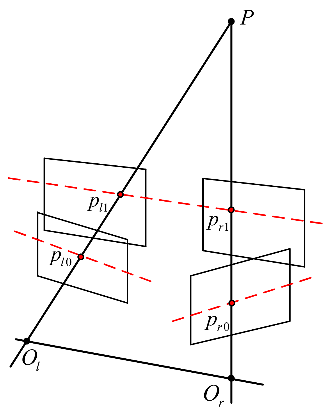
Stereo image rectification comprises image transformations, assuring that the corresponding epipolar lines in both images become collinear with each other and with the image scanning lines. Additionally, in rectified images, the optical axes are also parallel. The stereo vision system, which fulfils these conditions, is called a standard or canonical stereo setup. Its most significant advantage is that all the corresponding image features lie on the same lines in both images (see
Figure 2). Consequently, the search space is restricted to one dimension only, which is a very desirable feature from the computational point of view.
The rectification process includes the following transformations:
- –
rotation of the left and the right image to move the epipolar points to infinity, described by the matrix ,
- –
rotation of the right image by a matrix .
Additionally, without loss of generality, the following assumptions are adopted:
- –
the focal lengths of the two cameras are the same,
- –
the origin of the local camera coordinate system is the principal camera point.
2.3.3. Stereo Correspondence
Stereo correspondence matches a three-dimensional point in the two different camera views. This task is simplified because the rectification step ensures that the three-dimensional point in both image planes lies on the same epipolar line. Consequently, the searching area is restricted to only one row of the image. What is more, considering that the location of the point is known in the left image, the coordinates of its counterpart are moved to the left in the right image.
In order to find corresponding points, two attempts can be implemented. Firstly, the image features can be detected in both images and then matched with the restriction that the points must lie on the same epipolar line. Secondly, the image feature can be detected in one image only, and then, its counterpart can be found using a block-matching technique. The former demands more computational time and is not suitable for the presented solution as the slow matching step is used to track points between successive video frames. Therefore, we decided to employ the latter, which facilitates real-time execution.
We tested three of the block-matching techniques in our work. The first one was based on the Normalized Square Difference Matching Method [
64] to find matching points between the left and right stereo-rectified images. Despite its quick response, it was not as reliable in low-texture underwater scenes. The second algorithm, called the Normalized Cross-Correlation Matching Method [
66], was a bit slower but provided higher reliability and accuracy in all underwater scenes. The third algorithm, the Correlation Coefficient Matching Method [
67], yielded the most accurate matchings. Even though it was slower compared to the first two techniques, its computational time matched the assumed time restrictions. Consequently, it was the best fit for the proposed method.
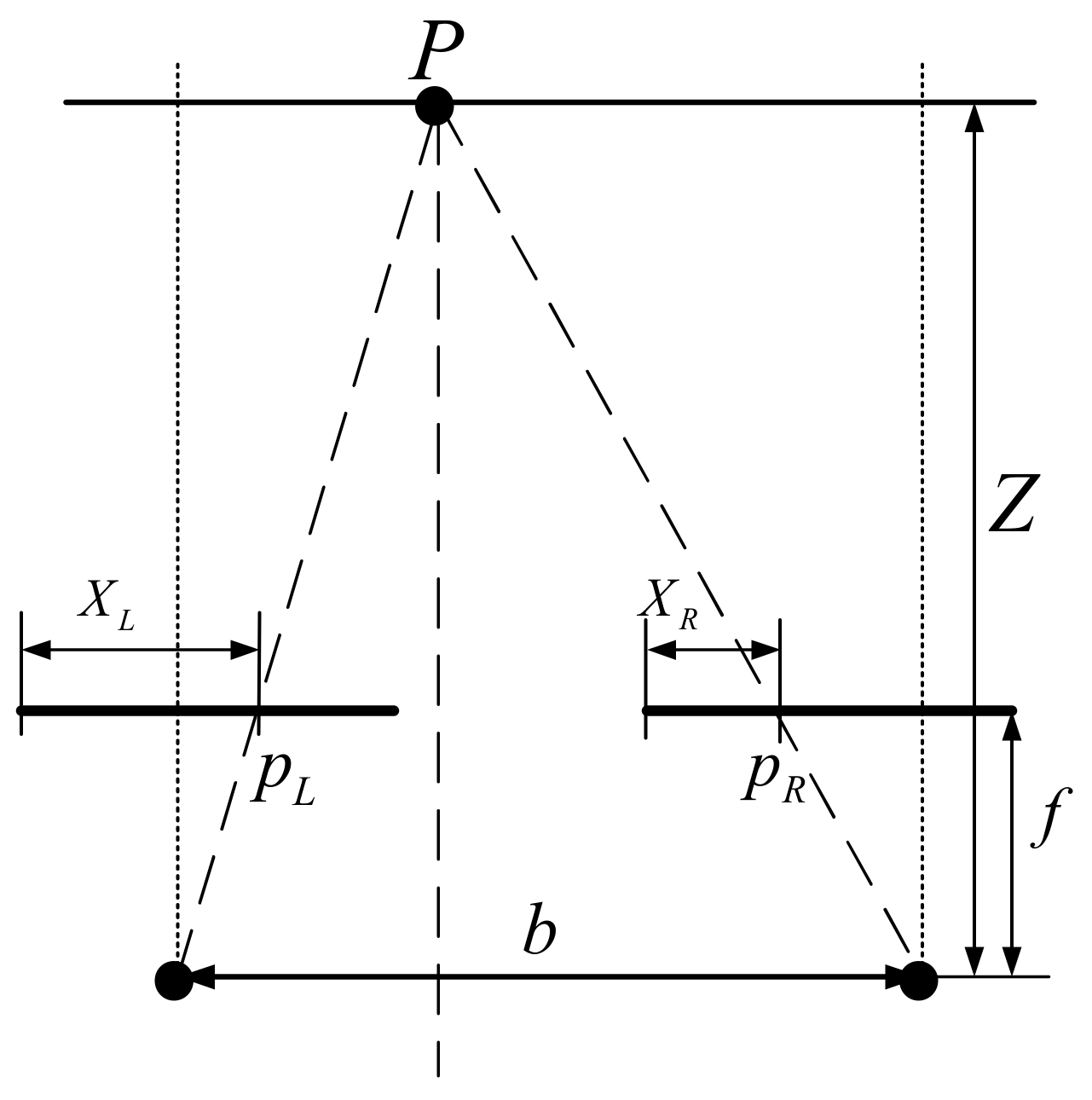
2.3.4. Triangulation
The triangulation task is simplified as the distortion removal and rectification steps were implemented in the method. Consequently, the stereo setup comprises two cameras whose image planes are coplanar with each other; the optical axes are parallel, and the focal axes are equal. Additionally, the principal points are calibrated and have the same pixel coordinates in the left and right images. This type of stereo setup, called the standard or canonical setup, is presented in
Figure 3.
In this case, the distance to the 3D point can be calculated from the following formula:
where
is the distance from the point
to the baseline,
is the distance between the cameras, and
is the camera focal length.
signifies horizontal disparity and is calculated as
, whereby
,
are horizontal coordinates of the points
and
on the image planes.
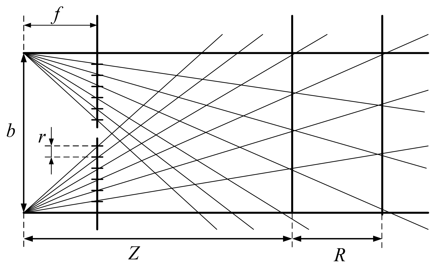
2.3.5. Distance Measurement
Distance measurement depends on the geometric parameters of a stereo vision system. In terms of accuracy, the following parameters are taken into consideration:
- –
focal length,
- –
distance between cameras,
- –
CCD resolution.
Figure 4 depicts the geometrical dependencies among the above parameters. Using the triangle similarity theorem, the equation describing geometrical dependence can be formulated as follows [
68]:
where
is measurement uncertainty,
is pixel size,
is distance measurement, and
is the distance between cameras.
The formula indicates that the increase in pixel size and the greater distance from the 3D point impair measurement accuracy. The measurement accuracy can be improved by increasing the focal length or the distance between the cameras. However, in this case, the minimal measured distance is extended.
In addition to the accuracy, there is the need to consider the stereo vision system on ROVs that can detect and match enough numbers of image features. For that reason, we performed analyses and simulations, which have been elaborately described in [
69]. Therefore, in this paper, we only indicate the main assumptions and exemplary results.
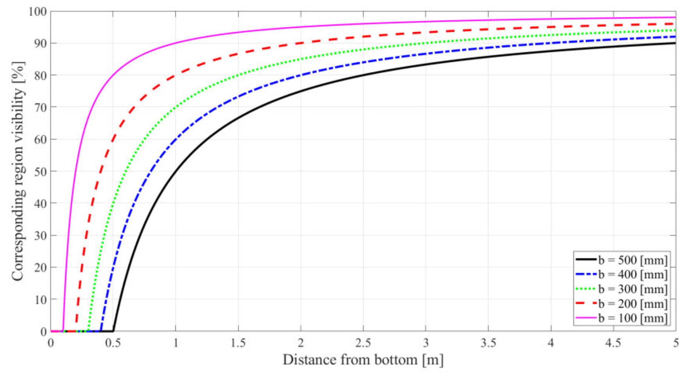
For detecting and tracking a sufficient number of image features, the following expectations were developed:
- –
the distance between the cameras, b, and the distance between the vehicle and the bottom, h, should assure a 75% visibility of the corresponding region in both images;
- –
the velocity of the vehicle in the forward direction, the distance from the bottom, and the frame rate of the image acquisition system should assure 75% visibility of the same region in the consecutive frames.
In case of the distance between cameras, the corresponding region of visibility for a camera with focal length f = 47.5 mm and image resolution 768 × 576 pixels for different baselines is presented in
Figure 5. As can be seen, all the considered baselines meet the requirements at a distance of 2 m from the bottom. For shorter distances, the length of the baseline should be adequately reduced.
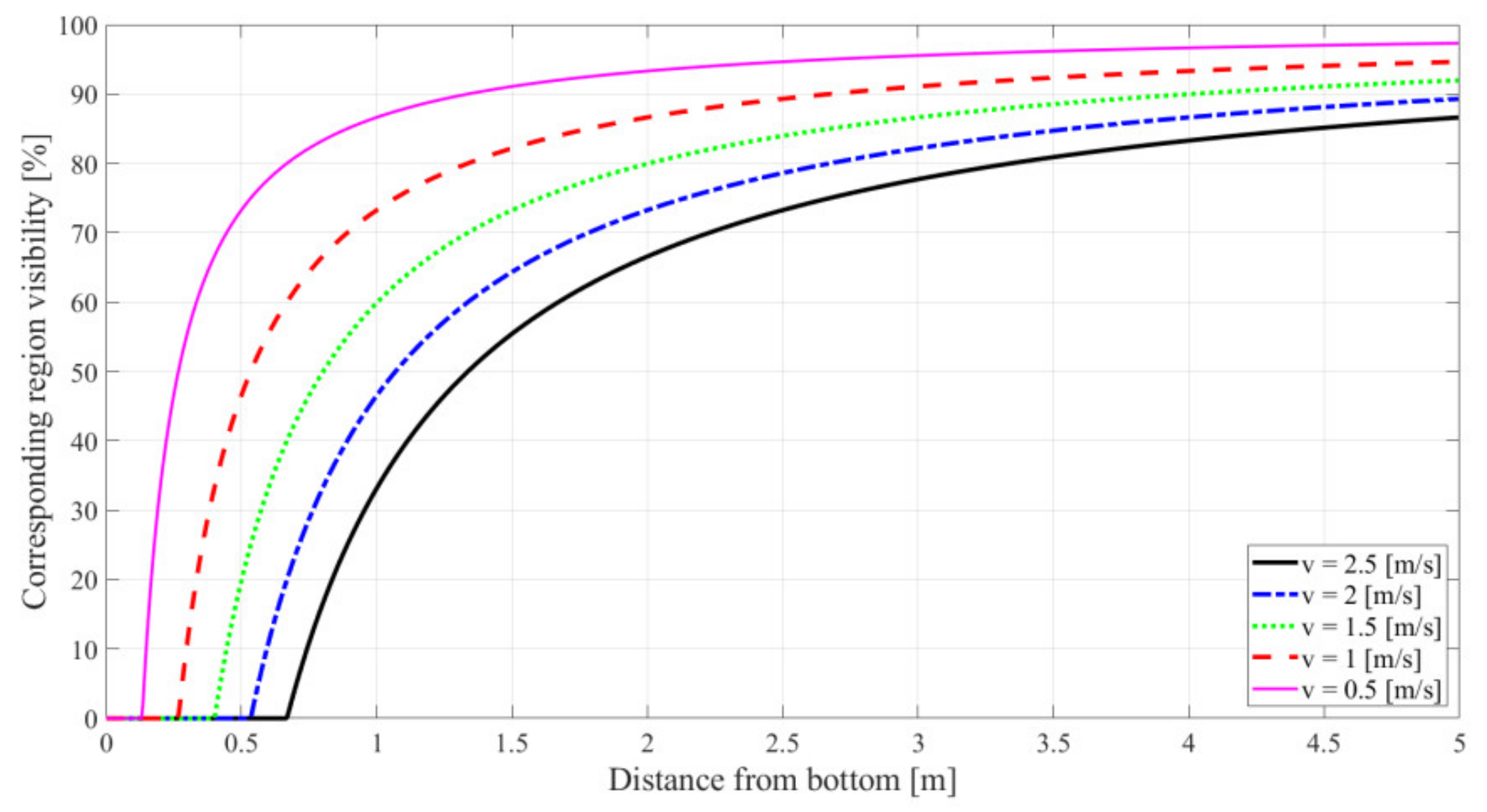
The relation between the distance from the bottom and the region of visibility, occurring in consecutive frames of the left camera, delineating the vehicle’s various velocities, is presented in
Figure 6.
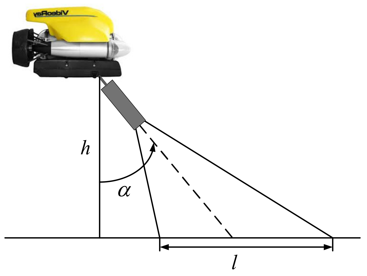
In this case, for the focal length f = 47.5 mm, acquisition rate = 5, and image resolution 768 × 576 pixels, the vehicle should move at a distance of 3 m from the bottom to meet the required 75% correspondence for all speeds. Additionally, taking into consideration the fact that the camera can be mounted at the angle
to the vehicle (see
Figure 7), the value of the angle also influences the corresponding region of visibility.
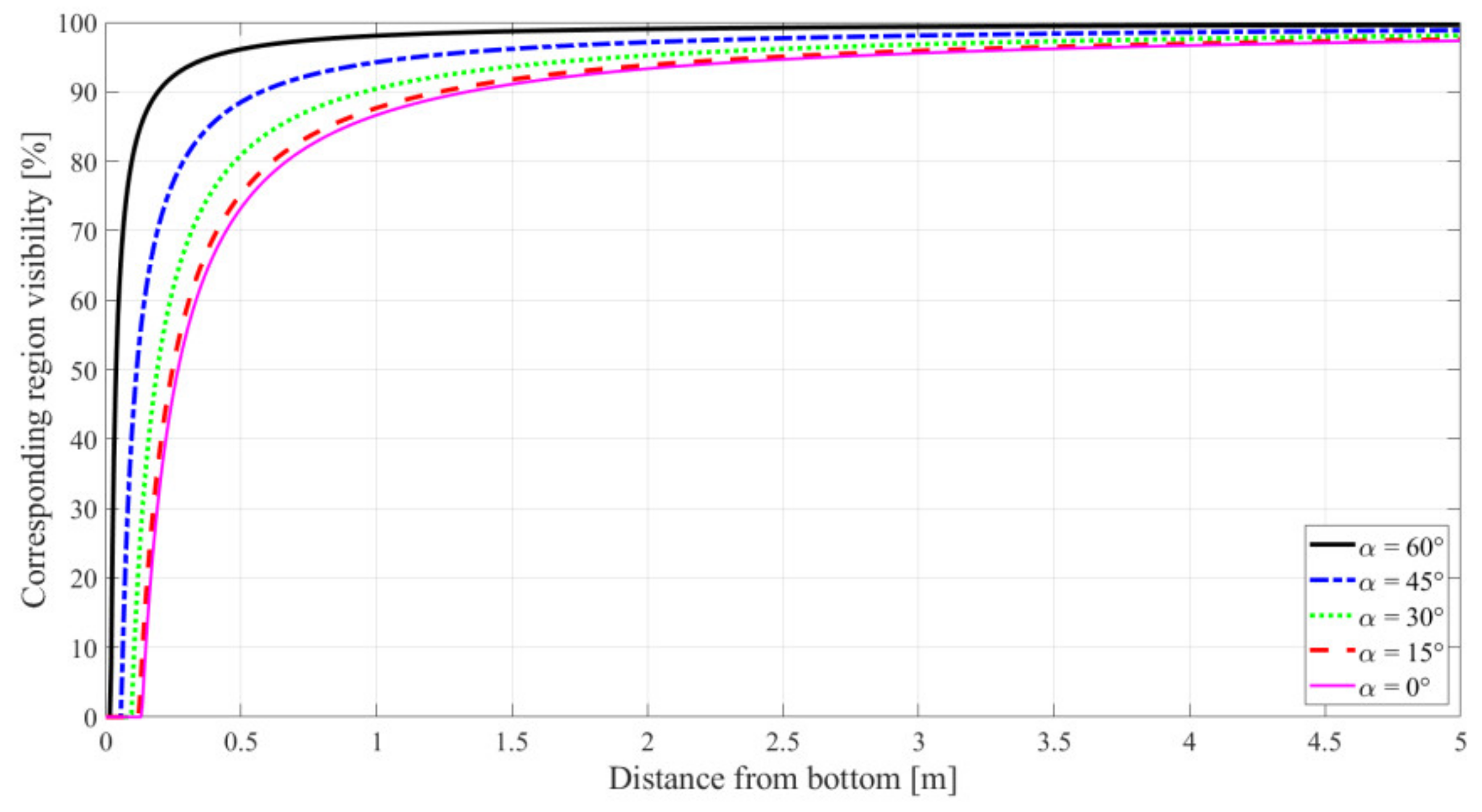
Figure 8 shows the relation between the corresponding region of visibility and the distance from the bottom for different angles
. The other parameters are the following: baseline = 300 mm, focal length = 47.5 mm, velocity = 0.5 m/s, and acquisition rate = 5.
The obtained results indicate that the demanded corresponding region of visibility for the established parameters in successive frames can be reached at a distance from the bottom that equals from 0.2 to 0.6 m, depending on the angle .
The conclusions from the conducted research point out that all the parameters should be considered together because, in the case of changing one of them, the other should also be adjusted. Consequently, for the established approximate distance from the bottom and the maximum velocity of the vehicle, the stereo vision system’s setting needs to be determined.
2.4. Image-Based Motion Calculation
In our research, we assumed that the vehicle moves at a close distance from the bottom and captures images using a stereo-vision setup. The period between the acquisition of the new stereoscopic images is shorter than 200 milliseconds. For each pair of the stereo images, the following steps are applied:
- –
distortion removal,
- –
rectification,
- –
detection of image features in the left image,
- –
stereo correspondence to find counterparts for detected image features in the right image,
- –
triangulation, to find distances from the bottom for matched image features,
- –
image-feature correspondence in successive frames of the left camera.
These steps allowed us to calculate the distances from the detected 3D points and analyse their positions in the consecutive frames. As camera motion along and about the different degrees of freedom causes different movements of feature images, analysis of this movement provides information about the velocity of the camera
:
where
is the translational velocities (surge, sway, heave),
is the rotational velocities (roll, pitch, yaw).
For a camera moving in the world coordinates frame and observing the point
with camera coordinates
, the velocity of the point relative to the camera frame is [
69]:
which can be rewritten in scalar form as:
Taking into consideration the normalised coordinates of a point on the image plane:
and applying the temporal derivative, using the quotation rule:
the relation between the velocity of the image features and the velocity of the camera can be formulated as:
and reduced to the concise matrix form:
where
is the Jacobian matrix for an image feature.
The motion of the three image features may be considered by stacking the Jacobians:
Assuming that the image features are not coincident or collinear, the Jacobian matrix can be regarded as non-singular. Consequently, the velocity of the camera can be calculated using the following formula:
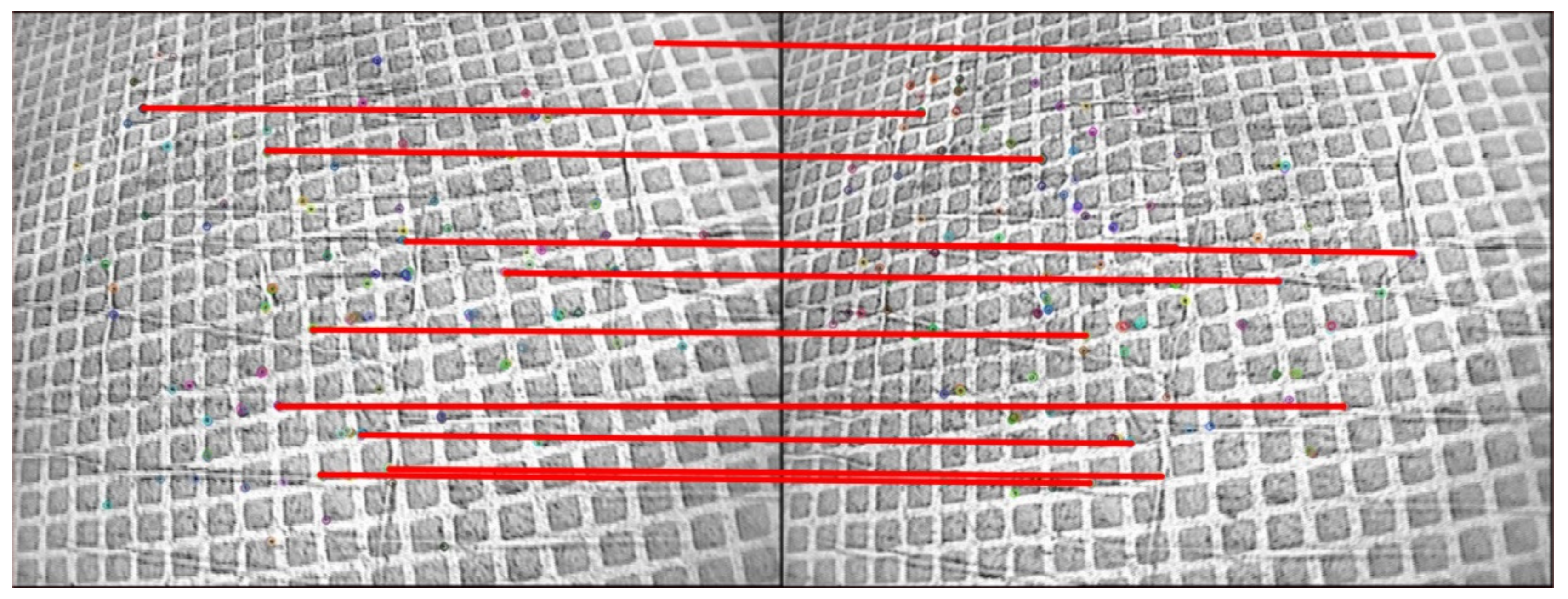
The formula indicates that only three correspondences between the feature points in consecutive frames are needed to calculate the six velocities. However, during the execution of the algorithm, the number of matched features is usually higher than 10. Therefore, the least-squares method for solving the system of equations was implemented.
Figure 9 depicts an example of feature points matching on consecutive left camera frames for the velocity calculation.
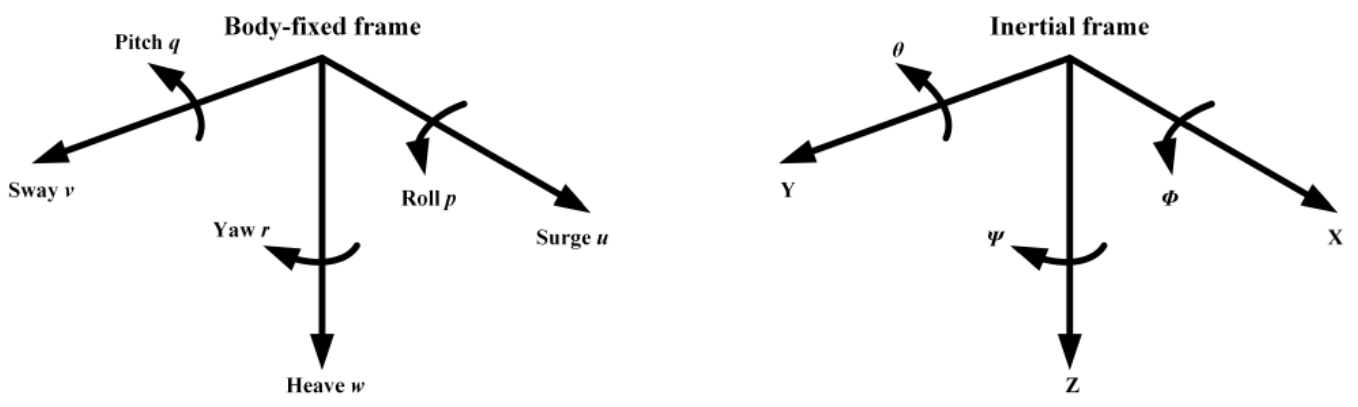
The velocity of the camera facilitates the calculation of the vehicle’s speed. To perform this calculation, the body-fixed and the inertial-fixed frames, presented in
Figure 10, were adopted.
The motion of the body-fixed frame is described in relation to an inertial reference frame. At the same time, the linear and angular velocities of the vehicle are expressed in the body-coordinate frame. The translational velocity of the vehicle, described in the body-fixed frame, is defined as translational velocity in the inertial frame through the following transformation [
70]:
where
Similarly, the rotational velocity in the inertial frame can be expressed using the rotational velocity of the vehicle as [
71]:
for the transformation
:
where:
—,
—,
—
In our work, a compass and an IMU (Inertial Measurement Unit) support a vision system because they provide the heading of the vehicle as well as its position relative to the inertial frame, expressed as roll
, pitch
, and yaw
(see
Figure 8). This information facilitates the calculation of the translational and rotational velocity in the inertial frame using Equations (22)–(25). Additionally, as the stereo-vision setup’s coordinate frame needs to be transformed into the vehicle’s coordinate frame, the transformation is achieved utilising Equations (22)–(25) for
and
.
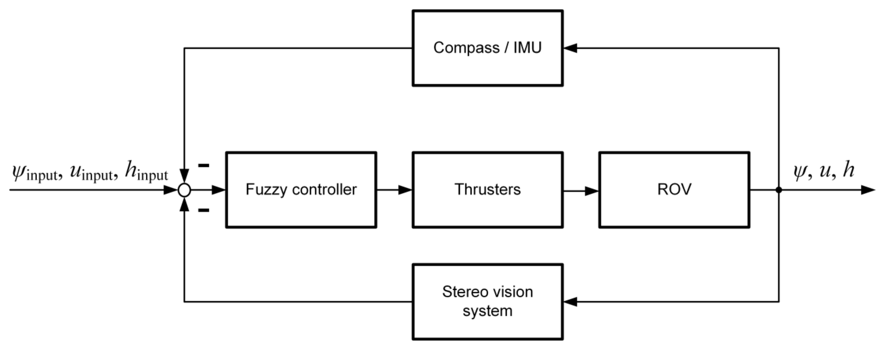
2.5. Control System
A control system, developed to implement the stereo-vision technique into the control process, is presented in
Figure 11.
In this solution, the compass measures the heading of the vehicle. At the same time, a stereo vision system determines the motion of the vehicle in the x-direction (surge u) and the distance from the bottom h. The measured values are compared with the desired ones, and the obtained differences are passed to the controllers. The type of the controllers can depend on the ROV’s dynamics, but for many applications, fuzzy logic controllers are the best choice for underwater vehicles due to their high nonlinearity and nonstationarity.
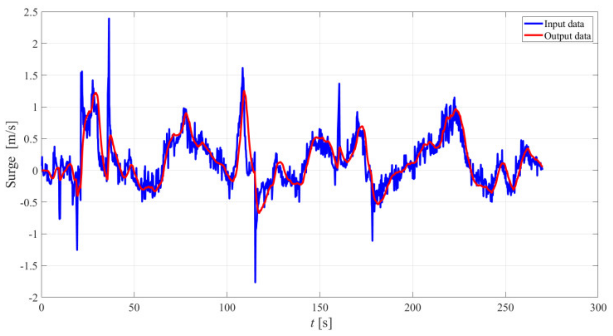
The preliminary experiments indicated that noise affected the values measured by the stereo vision system. The noise was attributed to the discrete character of an image and the inaccuracies during image-feature localisation. Therefore, to ensure the accuracy of the measurement, the Kalman filter was employed in the control loop. Based on the experimentations, our solution had the following parameters of the filter determined:
- –
the state-transitional model of the surge motion and distance from the bottom:
- –
the observational model of the surge motion:
- –
the covariance of the process noise of the surge motion:
- –
the covariance of the observation noise of the surge motion
- –
the observational model of the distance from the bottom:
- –
the covariance of the process noise of the distance from the bottom:
- –
the covariance of the observation noise of the distance from the bottom .
The obtained result for the surge motion, presented in
Figure 12, indicates that the Kalman filter reduces noise generated by the stereo vision system very effectively.
3. Results and Discussion
The proposed method was developed to facilitate control of the ROVs at a close distance from the bottom using visual information. As this method is regarded as a practical solution, we aimed to develop and test it, considering the real imaging conditions. Therefore, we carried out extensive research devoted to image-feature detection in various regions of future operations and under different lighting conditions. Consequently, as the most promising methods were determined using videos acquired during various ROV missions, we decided that the control system would be tested in a swimming pool. This solution was convenient because it allowed for a precise measurement of the displacement of an ROV, which would be very challenging in the real environment.
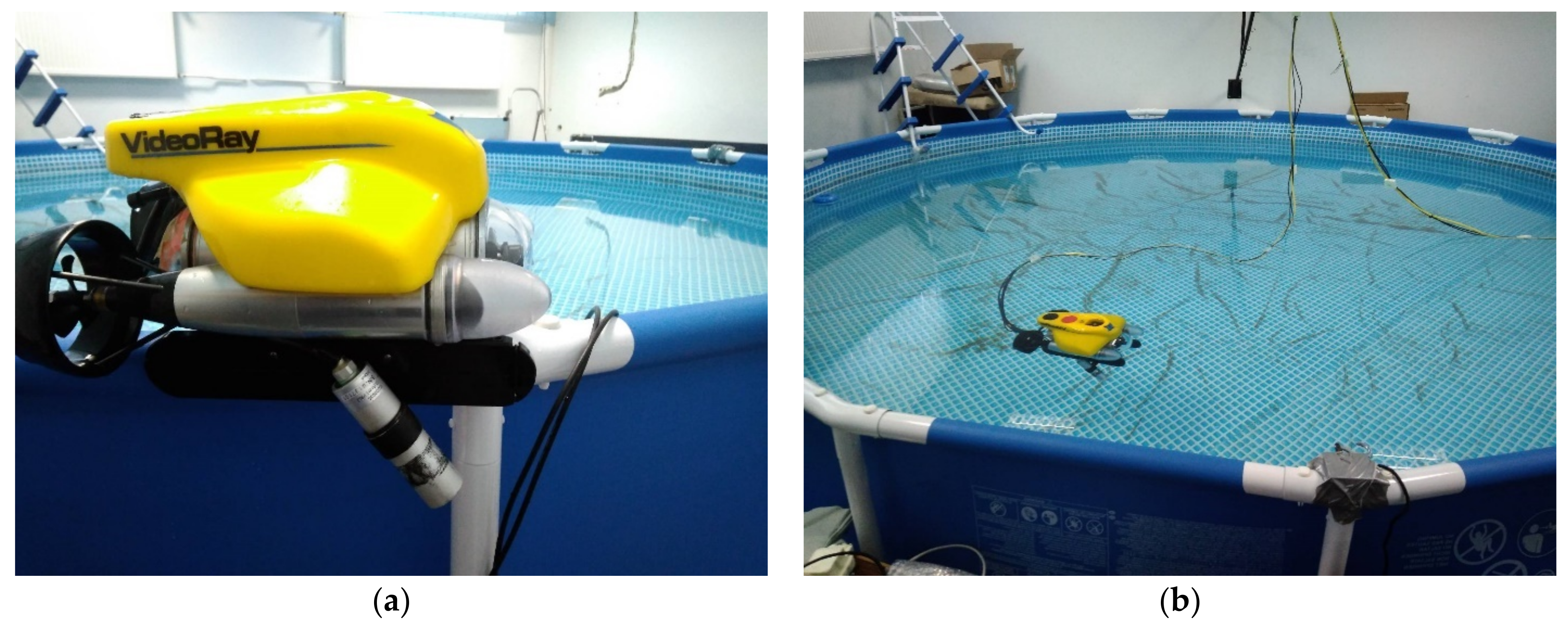
The experiments were conducted using a VideoRay Pro 4 underwater vehicle and a small inspection-class ROV (see
Figure 13), implemented in plenty of applications worldwide. It carries the cameras, lights, and sensors to the underwater places wanting to be observed. The vehicle is neutrally buoyant and hydrostatically stable in the water due to its weight distribution. It has three control thrusters, two for horizontal movements and one for the vertical one; therefore, the vehicle’s control is only available in the surge, heave, and yaw motion. Equal and differential thrust from the horizontal thrusters provides control in the surge and yaw motions, respectively, while the vertical thruster controls the heave motion.
The VideoRay Pro 4 utilises the ADXL330 accelerometer and the 3-axes compass, which provide information about the heading of the vehicle as well as the roll, pitch, and yaw angles. Additionally, we equipped it with two Colour Submergible W/Effio-E DSP Cameras with a Sony Exview Had Ultra High Sensitivity image sensor, constituting a stereo-vison setup. The cameras and the vehicle were connected to a computer with Intel Core i7-6700HQ CPU 2.6 GHz and 32 GB RAM. The computer served as the central computational unit for the developed algorithms.
To conduct the experiments, a vision-based measuring system described in [
45] was utilised. The system allowed the vehicle’s position determination with an error of fewer than 50 millimetres, which constituted a satisfying precision. Apart from position determination, the vision system allowed for the time measurement needed for the vehicle’s speed and heading calculation. A built-in pressure sensor in the VideoRay Pro 4 vehicle was used for measuring depth control. Its accuracy was estimated during hand-made measurements and indicated that the error was less than 20 millimetres. This error value was relatively small and did not influence the performed analyses.
The vehicle was marked with a red circle. Through the segmentation based on a red colour separation, the circle was detected by the vision-based measuring system [
45]. The system enabled the vehicle’s position determination using a camera mounted below the ceiling. During experiments, the vehicle’s position was recorded to the file with the interval equal to 75 ms. At the same time, the applications devoted to communicating with the vehicle sent control signals and received the vehicle’s depth and heading with the interval equal to one loop of execution of the proposed algorithm. As both applications were running on the same computer, the sent and obtained data were stored in the same file, which facilitated further analyses.
The presented method was compared with the SLAM techniques based on the ORB-SLAM and ORB-SLAM2 systems [
16,
17,
18]. ORB-SLAM and ORB-SLAM2 are state-of-the-art SLAM methods that outperform other techniques in terms of accuracy and performance. Their usability was proved in a wide range of environments, including underwater applications. Additionally, their source code was released under the GPLv3 license, making implementation very convenient.
SLAM mainly utilises a monocular camera, which makes it prone to a scale drift. Therefore, the sensor fusion of a camera, lasers, and IMU were taken into consideration. The two parallel lasers are often used for distance calculation in ROV applications. Two points, displayed on the surface from the lasers mounted on the vehicle, enable simple distance calculation using Equation (1). For this calculation, only the camera parameters are required. The performance of the SLAM technique is also often improved by employing an IMU or utilising a stereo vision system. As a result, the most general problem of scale ambiguity is resolved.
3.1. Heading Control
To develop heading control, the fuzzy logic controller for the heading control was designed. In this process, we used the mathematical model of VideoRay Pro 4 and Matlab Fuzzy Logic Toolbox. Based on conducted experiments, we decided that the fuzzy logic PD controller using Mamdani-Zadeh interference would be the most convenient solution for our application [
71]. The defined memberships functions and the rule base are presented in
Figure 14 and
Table 1. It achieved a satisfying performance and did not require numerous parameters to be determined (in comparison with the PID fuzzy controller). The obtained results were verified during the experiments in a swimming pool, and some improvements to the controllers’ settings were introduced using input and output scaling factors. Finally, the scaling factors were set as follows: the error signal—0.02, the derivative of the error—0.01, and the output signal—1.
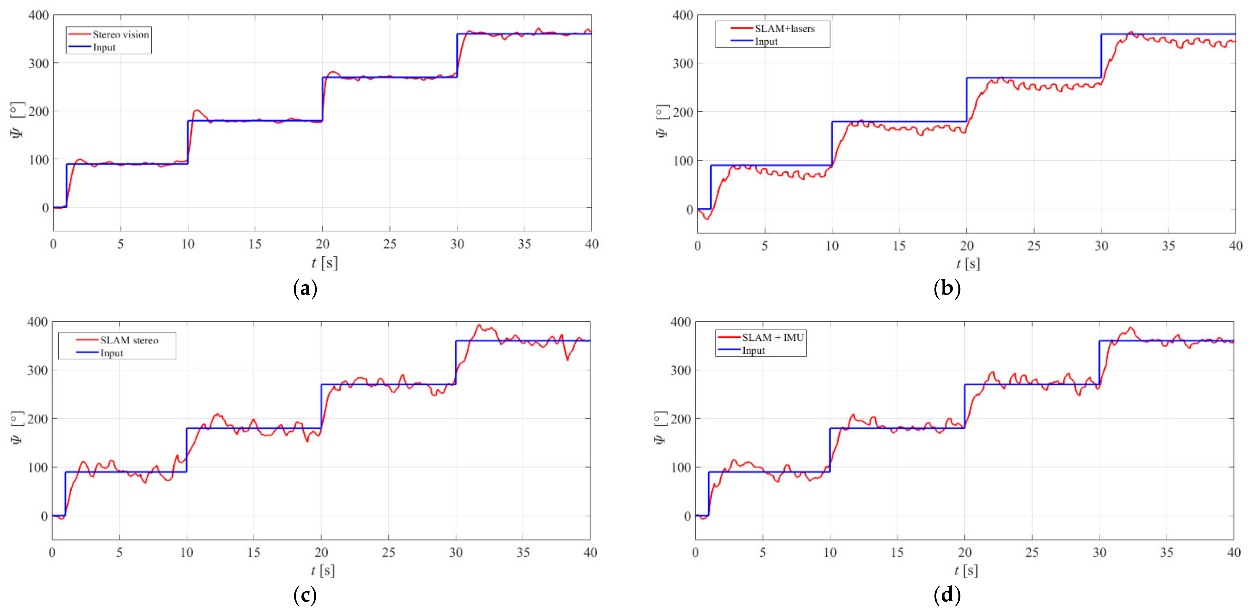
The analysed methods were tested for various speeds of the vehicle using different control strategies. First, the variable input signal was used. The vehicle’s heading was changed from 0 to 360 degrees for various vehicle speeds. The exemplary results for velocity equal to 0.1 m/s are presented in
Figure 15.
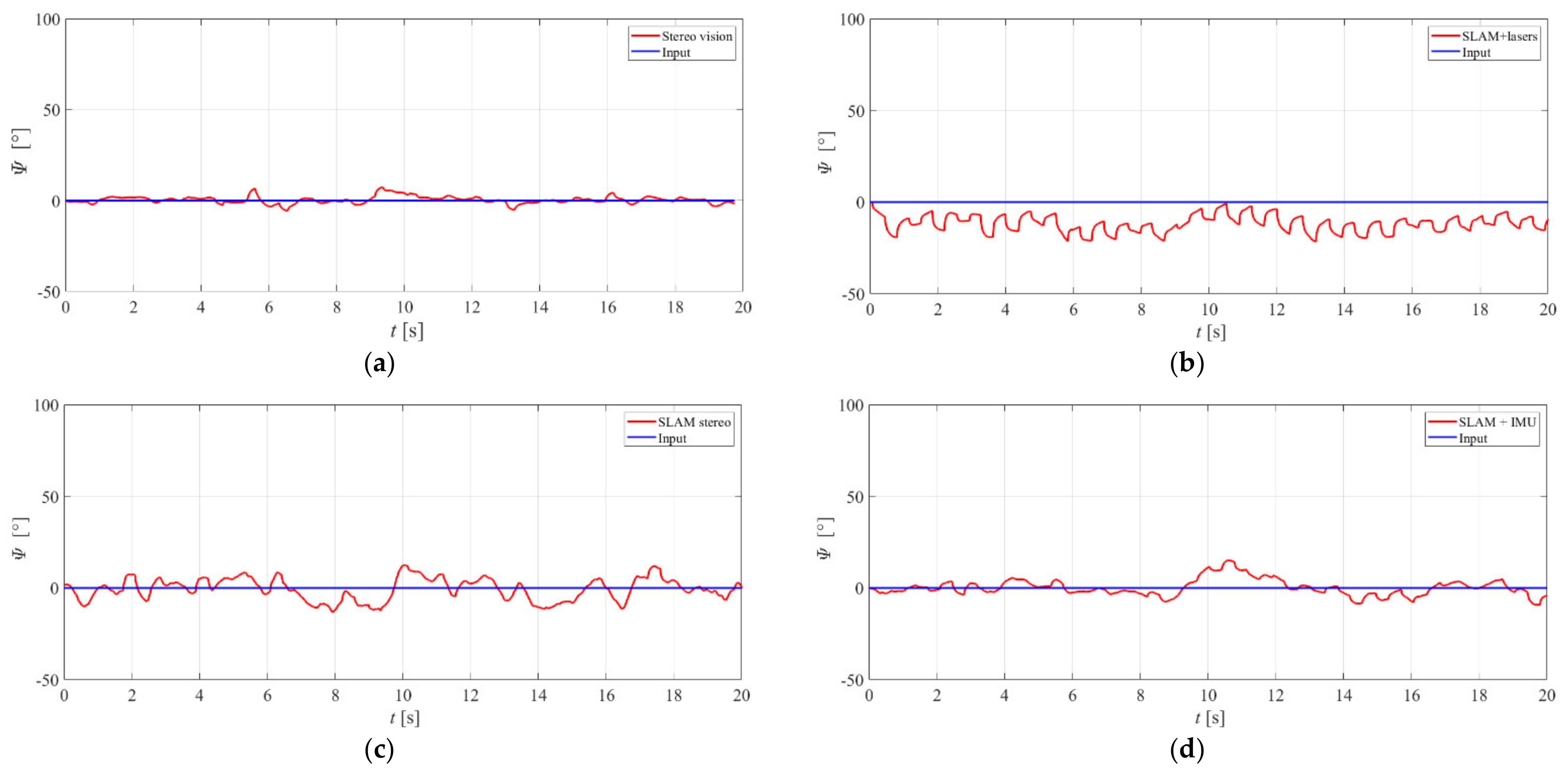
In the next part of the experimentation, the ability of the vehicle to keep a settled course was tested. During the tests, the vehicle moved at a constant heading for different speeds.
Figure 16 shows the obtained results for velocity equals 0.2 m/s.
The Integral of Absolute Error (IAE) technique was implemented for the comparison of the analysed methods. The obtained results are depicted in
Table 2.
They point out that our method outperformed others in the case of variable and constant headings. Slightly worse results for the variable headings were obtained using the SLAM IMU system, while the SLAM stereo and SLAM lasers delivered the worst performance.
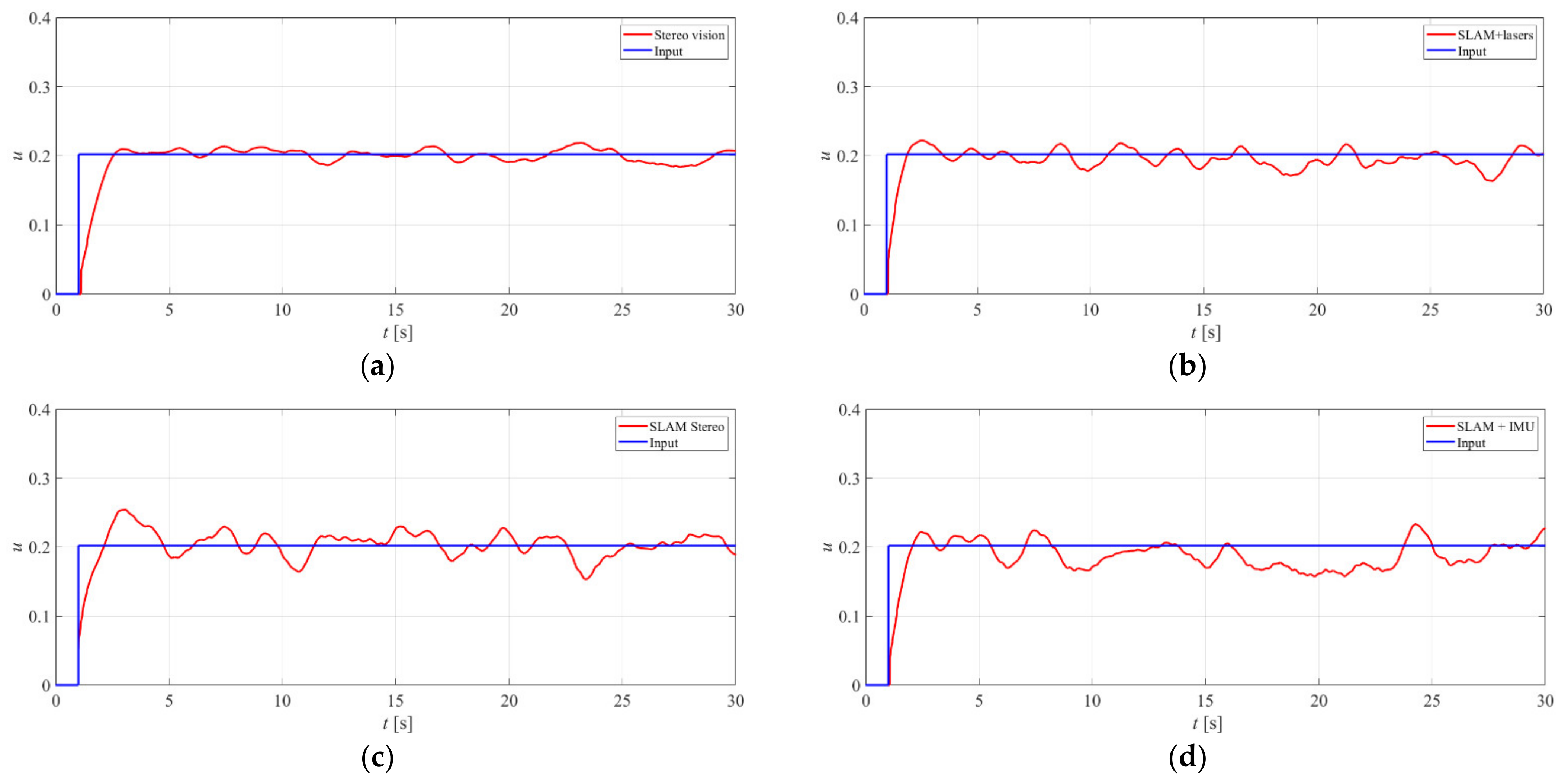
3.2. Surge Control
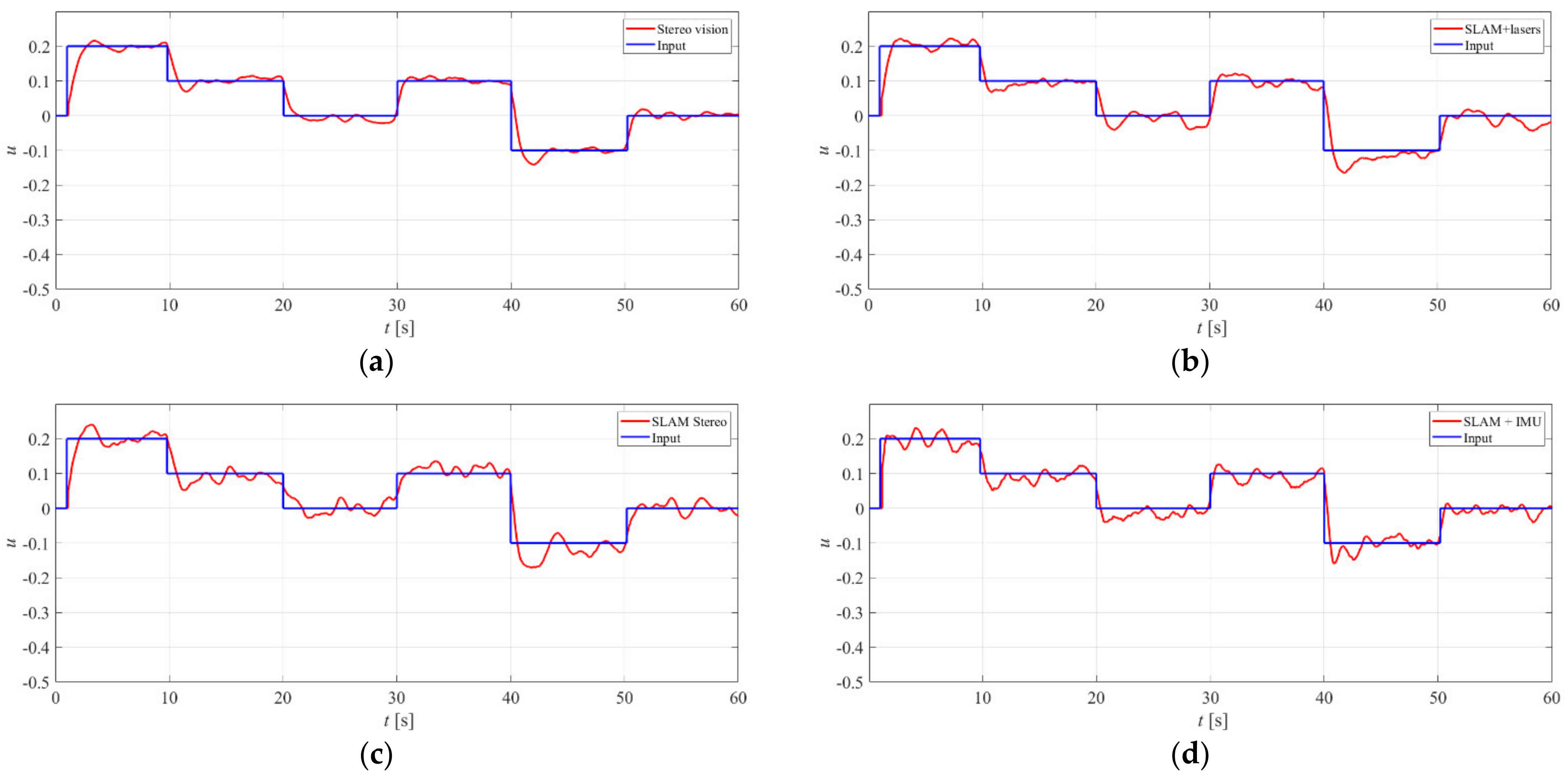
In case of surge control, similar to the previous experiments, the fuzzy logic PD controller using the Mamdani-Zadeh interference was implemented. (The same memberships functions and base rule as for the heading controller were adopted. The scaling factors were set as follows: the error signal—2, the derivative of the error—3, and the output signal—1.) The trials were performed for the variable and constant surge velocity. The results obtained for varied speed are presented in
Figure 17, while
Figure 18 shows the outcomes for constant speed equals 0.2 m/s.
Table 3 presents the Integral of Absolute Error calculation for the analysed methods.
The obtained results indicate that the proposed method allowed controlling the surge motion with high precision. Other methods facilitated less accurate control. Our observations indicated that even a small movement of the tether behind the vehicle affected its velocity considerably.
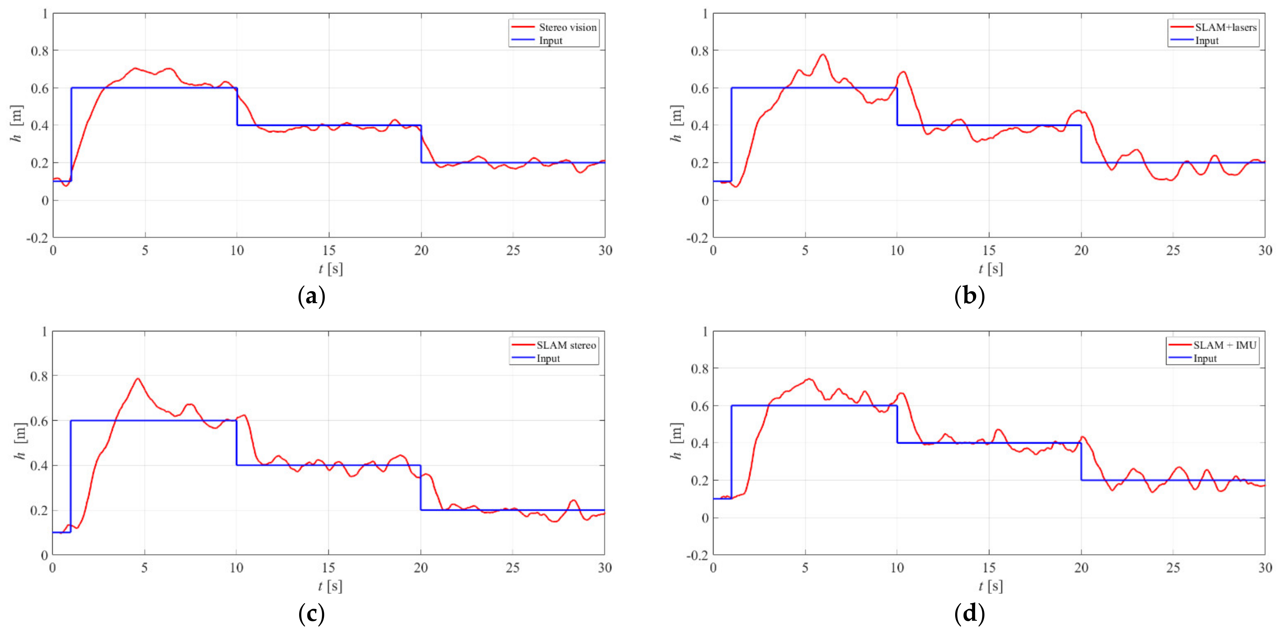
3.3. Distance-from-the-Bottom Control
The distance-from-the-bottom control system was assessed using a pressure sensor. At this point, it should be emphasised that the pressure sensor measures the depth of the vehicle, while the analysed methods compute the distance from the bottom. As the depth of the swimming pool was known, it was possible to calculate the distance from the bottom based on the vehicle’s depth. However, in most ROV applications, the exact depth of a water column is unknown, and information about the vehicle’s depth is insufficient to determine the distance from the bottom.
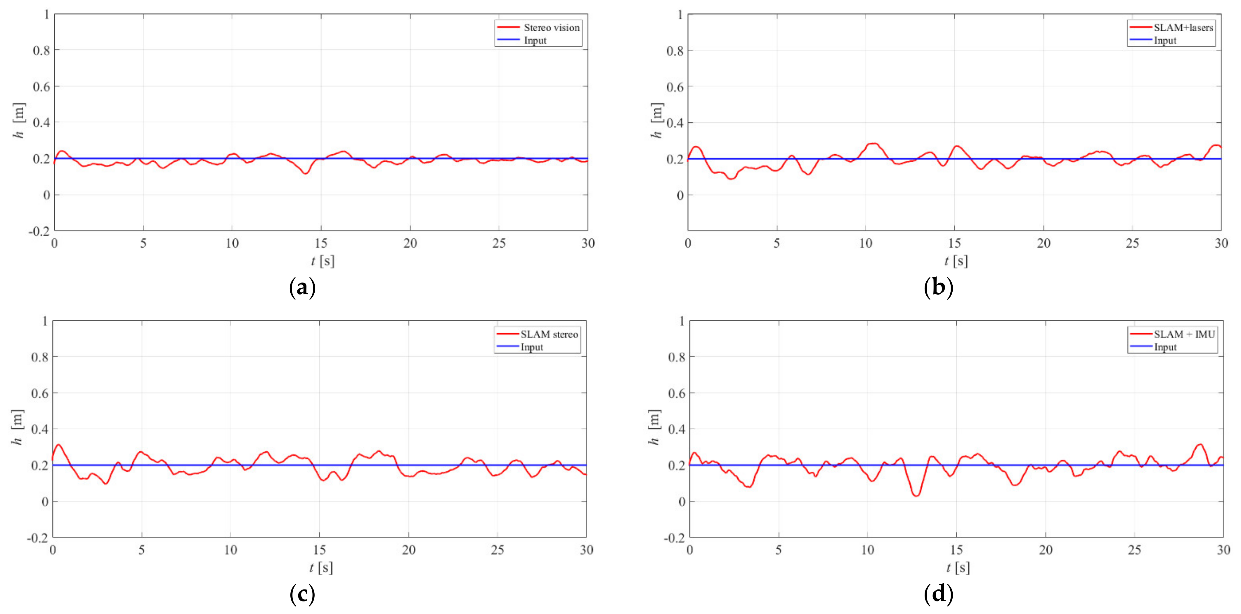
Similar to the previous experiments, the fuzzy logic PD controller using the Mamdani-Zadeh interference was implemented. (The same memberships functions and base rule as for the heading controller were adopted. The scaling factors were set as follows: the error signal—1, the derivative of the error—3, and the output signal—1.25.) During the experiment, we tested the developed controllers for various speeds as well as for constant and variable depths.
Figure 19 shows the results for variable depth and the vehicle’s speed equal to 0.1 m/s, while
Figure 20 depicts the results for constant depth and the vehicle’s speed equal to 0.2 m/s.
Table 4 presents the Integral of Absolute Error calculation for the analysed methods.
The obtained results show that our method obtained better results for variable and constant distance-from-the-bottom control.
The last part of the experiments was devoted to calculating the accuracy of the analysed method for variable speed, variable heading, and variable distance from the bottom at the same time. For the heading control, the vehicle’s heading was changed from 0 to 360 degrees for vehicle speeds from 0 to 0.2 m/s and distance from the bottom in the range of 0.2–0.6 m. In the case of surge control, the vehicle moved with the speed of 0–0.2 m/s with the heading in the range of −30—30 degrees and with the distance from the bottom in the range of 0.2–0.6 m. A similar range of parameters was used for the distance control. The obtained results are in line with the ones obtained in previous experiments (see
Table 5).
The performed analyses indicate that the proposed method enables automatic control of the ROV’s surge motion, and it maintains the calculated distance from the bottom. It also achieved better results in heading control in comparison to the analysed methods. This situation may stem from the fact that the proposed solution employs visual feedback in each control algorithm’s loop. In the case of SLAM and the SLAM techniques, the control loop can perform with the previous data when the new position is not calculated. The results obtained for the constant input signals are crucial for future applications as the vehicle is expected to move with a constant speed and distance from the bottom.
The mean computational cost of the analysed algorithms is presented in
Table 6. It has been measured for one loop of the algorithms. The results show that all the algorithms perform faster than 200 ms. It can also be noticed that the SLAM lasers and SLAM IMU are quicker than the stereo vision and SLAM stereo. This is because the SLAM laser and SLAM IMU need to analyse only one picture during execution.


