On Dispersion and Multipath Effects in Harmonic Radar Imaging Applications

Abstract

In harmonic radar applications, images produced using algorithms of conventional radar applications experience some defocusing effects of the electronic targets’ impulse responses. This is typically explained by the dispersive transfer functions of the targets. In addition, it was experimentally observed that objects with a linear transfer behavior do not contribute to the received signal of a harmonic radar measurement. However, some signal contributions based on a multipath propagation can overlay the desired signal, which leads to an undesired and unusual interference caused by the nonlinear character of the electronic targets. Here, motivated by the analysis of measured harmonic radar data, the effects of both phenomena are investigated by theoretical derivations and simulation studies. By analyzing measurement data, we show that the dispersion effects are caused by the target and not by the measurement system or the measurement geometry. To this end, a signal model is developed, with which it is possible to describe both effects, dispersion and multipath propagation. In addition, the discrepancy between classic radar imaging and harmonic radar is analyzed.

1. Introduction

Harmonic radar is a niche microwave measurement technique that enables new detection capabilities, especially in security related applications. In the past, research activities where focused on the detection of electronic devices such as mobile phones, for instance [1,2]. These devices are not intended to show a nonlinear behavior with respect to the interaction with an impinging electromagnetic signal. However, due to the possible presence of nonlinear circuit-elements within the target devices, such a behavior could be excited, given a sufficient electric field strength. A possible application of this particular detection scheme could be a security gateway or a luggage scanner at an airport or the entrance of a company building, where certain restrictions on the presence and use of electronic devices are to be enforced. More recently, a novel harmonic radar system for maritime safety applications was presented. This system is designed to work in conjunction with a known and matched transponder attached to a life-jacket [3,4]. Other applications with known target devices include the tracking of insects and small animals [5,6] or the detection of avalanche victims [7].

The aforementioned examples illustrate how harmonic radar can be applied. Besides the specific measurement systems and the targets that are to be located, the algorithms used for deciding whether a target is present or not, and if so, where it is located, play a key role in the performance and usefulness of the whole harmonic radar scheme. For the detection of unknown targets, the method of choice is to compute pseudo-reflectivity maps using known and well-established imaging algorithms from conventional radar (e.g., the backprojection algorithm) [1,8,9]. From these images, a human operator would then be able to read out the desired information. One important advantage of this approach is that the harmonic radar images generated in this way are comparable to conventional radar images.

To justify the conventional imaging approach, a polynomial approximation in place of the true nonlinear target transfer function, together with a sinusoidal transmit-signal, is made [1,10,11,12]. Some dynamic effects might be additionally explained by incorporating dedicated frequency-dependent but linear circuit blocks [13]. From this analysis, it follows that the received signal at one frequency harmonic can be viewed, as if an already frequency multiplied signal would have been transmitted, which is then reflected at a point-like classic surrogate in place of the electronic target. With a step-wise sweep of the transmit-signals’ frequency, a discrete spectrum of the frequency-domain (harmonic) impulse response is generated. The subsequent treatment and processing of the harmonic data is then done at the chosen frequency multiple of the fundamental transmit-frequency.

This point of view and mathematical treatment of the harmonic radar measurement was proven to result in usable images. However, strong defocusing effects of the electronic targets’ two- or three-dimensional point-spread-function were observed [1,8,9]. These defocusing and dispersion phenomena are neither intended nor wanted and decrease the quality of the image material. The defocusing could be explained by the circumstance, that an electronic device does not act as an ideal frequency multiplier. Time delays caused by internal signal propagation-paths, as well as possible frequency-dependent transfer functions introduced, e.g., by filter elements in a Bluetooth or WiFi receiver, should result in a dispersive and nonlinear transfer behavior.

Describing nonlinear electronic circuit elements is known in the engineering literature. There exist some methods to treat these devices similar to S-Parameters [14]. One of the more widely known descriptions are X-Parameters [15] or the poly-harmonic distortion modeling [16]. These methods are useful for describing interconnected dynamic nonlinear circuit elements, for instance, but are not used in harmonic radar applications.

Another aspect in harmonic radar is the influence of surrounding objects and the measurement environment, both viewed as having a strictly linear scattering behavior. These scattering-elements do not generate harmonic signal components themselves, and therefore do not contribute directly to the received signal. As a consequence, no well-focused traces should be visible in harmonic radar images. The conclusion that could be drawn from this is, that harmonic radar images are free of clutter, which was also observed experimentally [9,17].

The aforementioned arguments and observations are correct. However, one aspect is not included. The environment does not produce frequency multiples itself, but is scattering the harmonic signals emitted by the electronic targets. Furthermore, the transmit-signals at the fundamental frequency are also impinging through multipath channels on the electronic targets. Compared to a classic radar scenario, the only multipath contributions not present are the ones ranging from the transmit-antenna via the environment to the receiver. Of particular interest are the transmitter—environment—target multipath channels, as they overlay with the desired transmitter—target signal. Due to the following nonlinear transfer function applied to this compound signal, an intermixing and disturbance of both signals can be expected.

It is not possible to capture and explain all dynamic nonlinear effects with a simple polynomial approximation of an assumed frequency-independent nonlinear transfer function. The influence of the multipath propagation caused by the scattering environment is also not included in the models found in the literature. To explain and mathematically describe this circumstance and physical phenomena, a nonlinear interaction and propagation model for harmonic radar applications is developed and presented in here. With this, the mentioned phenomena are analyzed using simulation studies. In particular, the separate treatment as well as the influence on each other are investigated.

The proposed signal and measurement model is based on a Volterra series representation of the frequency-dependent, dynamic, and nonlinear target transfer functions [18,19]. The Volterra series generalizes the Taylor series, which only describes static nonlinear system functions, to a frequency dependent nonlinear transfer behavior. This circumstance makes it a powerful tool in describing general dynamic nonlinear systems, as it is necessary in harmonic radar applications.

The Volterra series is known and used in electromagnetic problems and circuit theory. In [20], this approach is used to model ultra-high frequency (UHF) receiver front-ends for communication and television applications, whereas in [21], methods for estimating the Volterra coefficients of radio-frequency power amplifiers are summarized. In [22], Sarkar et al. are describing a method for modeling and analyzing antenna structures with non-linear loads.

Here, we approach the task of developing a dynamic nonlinear target model, including the wave propagation to and from the harmonic radar systems’ antennae, from a strict signal theoretic point-of-view. We do not incorporate individual circuit elements in the model, nor do we apply strict electromagnetic formulations. The target is viewed as a black-box with a dynamic nonlinear input-output relationship. The wave-propagation is described by simple amplitude and phase factors.

In conjunction with the derived Volterra and multipath model, some simple example systems composed using separate static nonlinear elements, as well as dynamic linear transfer-elements, are presented. Based on these special cases, simulation studies are performed and analyzed. For first simulations, simple and straight-forward random transfer function generators are developed and explained.

The theoretical derivations as well as the simulation studies are motivated by the analysis of measurement data. We observe that neither the measurement geometry nor the measurement system is causing the dispersion effects, but conclude that the electronic target itself is the reason for this observation.

The structure of this article is as follows. The experimental motivation for the theoretical derivations is given in Section 2 together with a detailed data-analysis regarding the dispersion and multipath effects as well as the theoretical analysis of the observed effects (the data used in here were previously published in our article [9]; here, we provide a more detailed analysis). In Section 3, the proposed Volterra and multipath model is derived and explained. The simulation study described in Section 4 concludes the main part of this article with a detailed analysis of the observations.

2. Experimental Observations and Analysis

In the following, we analyze our experimental results previously published in [9]. Here, the presented investigations are focused on the dispersion effects visible in the harmonic radar images, generated from raw-data using the backprojection algorithm. The experimental setup is briefly outlined. As a comparison, ideal synthetic data are generated using the same parameters as in the experiment.

2.1. Measurement and Simulation Setup

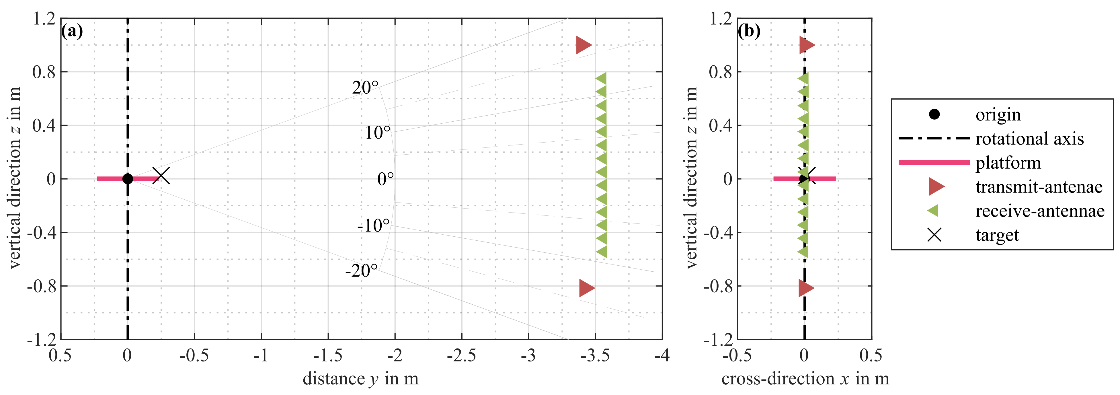
The measurement setup is explained in detail in [9], and is again illustrated in Figure 1, showing only relevant details. The key information is summarized in the following.

In principal, the measurement system follows a stepped-frequency continuous wave approach. For each discrete frequency point, a sinusoidal transmit-signal is generated and recorded in time-domain after a down conversion to a constant intermediate frequency of 30 MHz. In addition to the measurement signals, a comparison signal providing a phase reference is recorded. This signal is kept in a closed loop in the system. The relative phase and amplitude values at each selected frequency are then used for the signal processing and image generation steps. For the harmonic radar measurement, the frequency range is 2 to 3 GHz on transmit and 4 to 6 GHz on receive. The transmit-frequency range is divided into 33 equidistant and discrete frequency points. The transmit-power is approximately 20 W.

The antenna-array consists of 2 transmit- and 14 receive-antennae, arranged vertically with equal spacing. The transmit-antennae are the first and last elements in the array.

The harmonic test target is an improvised transponder, constructed using a mixer with an extended center conductor at one of the three ports acting as an antenna. The other two ports are loaded with 50 Ω loads. The measurement system and antenna-array are stationary. The test target is placed on a rotating platform, so that the measurement setup is comparable to an inverse synthetic aperture radar (ISAR) scenario. The constant distance of the array to the rotating platform is approximately 3.5 m. Measurements are obtained at 300 discrete and equidistant rotating angles of the target mounting platform with a total angular span of 360°.

The synthetic (simulation) data are generated using the parameters of the measurement, i.e., number of antennae, antenna placement, rotating angles, and approximate position of the test target and discrete frequency points. Deviating from the experiment, no time-domain signals are generated. The synthetic data used for the following signal processing and image formation steps are computed directly in frequency-domain. The synthetic test target does not show any frequency-dependent behavior, as it is used to obtain an ideal reference as a comparison to the experimentally obtained data and images.

2.2. Data Analysis

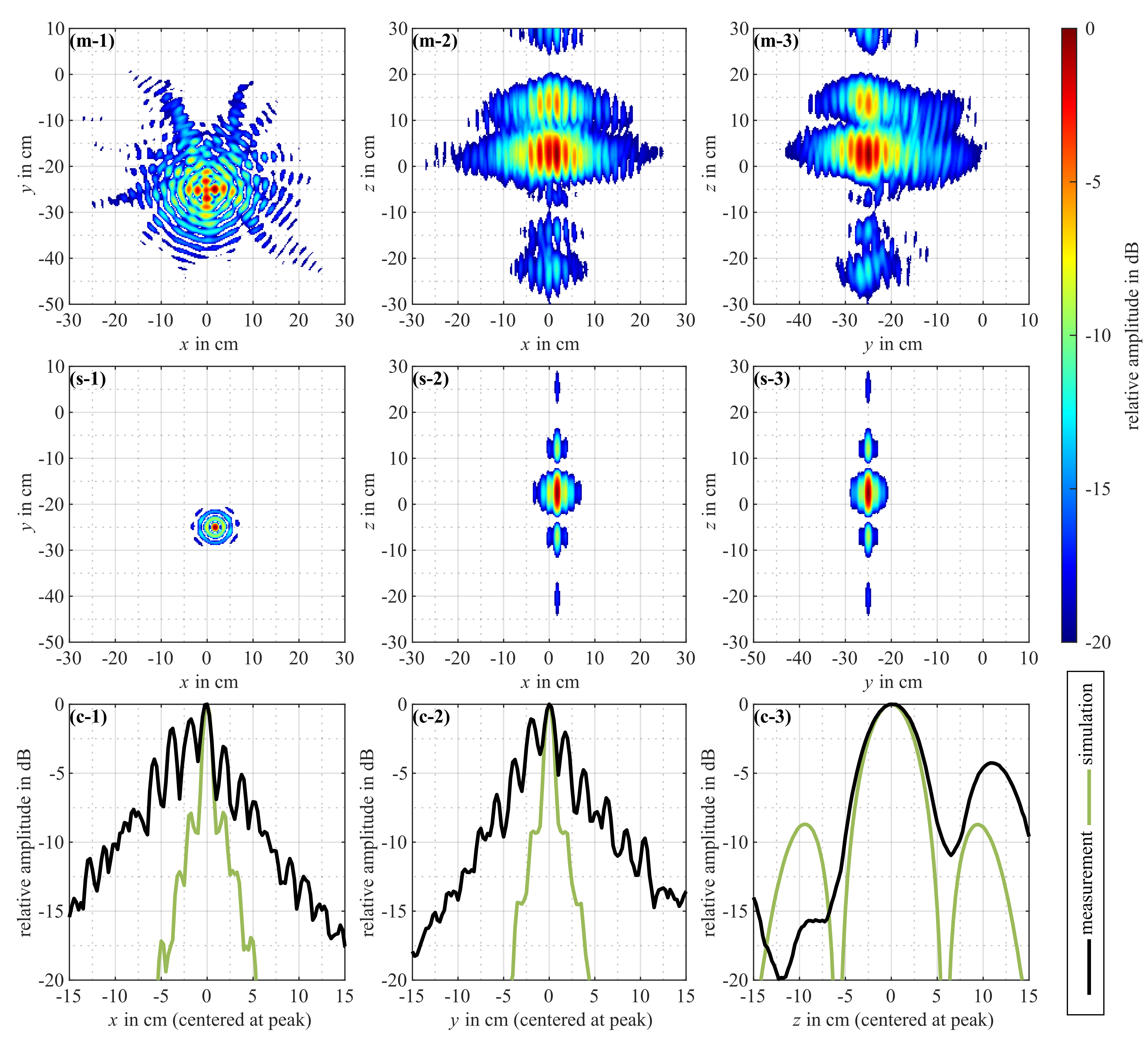
The images generated from the experimentally obtained data and simulations are shown in Figure 2. If not stated otherwise, all of the following references to images and graphs refer to this figure. The illustrations show two-dimensional maximum projections of a three-dimensional image cube, as well as one-dimensional maximum profiles. The images (m,s-1,2,3) cover an area of $60\times 60$ cm with the origin being located in the rotation center, aligned with the surface of the target platform. The profiles (c-1,2,3) span over 30 cm and are centered at the coordinate of the maximum value of the (m-1,2,3) images. This is approximately the true position of the harmonic test target.

The spatial image resolution is in the following defined as the full-width-at-half-maximum (FWHM) of the main-lobe of the maximum profiles obtained from the simulation data. In this case, the x– and y–resolution is 1.1 cm, and the z–resolution is 5.5 cm. As a comparison, the spatial-FWHM of a 2 GHz rectangular band-limited signal, as it is the case for the receive frequency window, is 7.5 cm. Due to the 360° viewing angles, the spatial frequency range in the xy–plane is significantly improved compared to the pure signal frequency range. The relative increase in the xy-resolution is 6.8. The limited angular range in z direction results in a relative z-resolution improvement of 1.4.

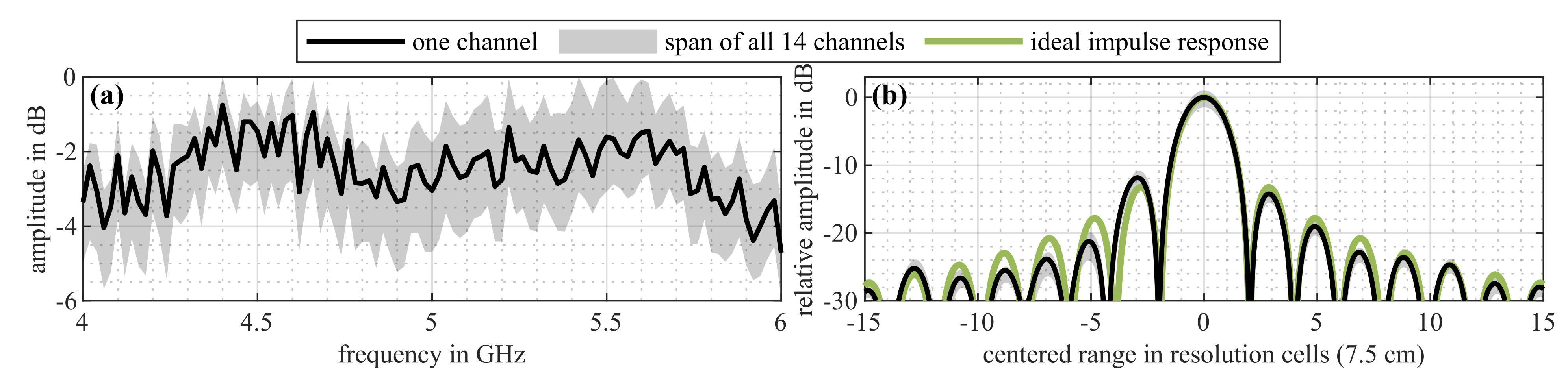
In [9] and Figure 3, the frequency-domain and corresponding spatial-domain transformations of the system calibration measurements are shown for all 14 individual receive-channels. The calibration data were obtained in a closed-loop measurement and contain the full receive- and transmit-paths, however, without the antennae and some connecting cables. The spatial-domain graphs shown in Figure 3—(b; —) match closely (in the range of 4 to 6 dB) with the ideal impulse response shown in Figure 3—(b; —). It should therefore be principally possible to produce almost dispersion-free images, assuming that other influences (e.g., antennae) are not degrading the systems’ impulse response.

A comparison of the ideal simulation-based images and profiles to the measurement results reveals a significant discrepancy in the image quality. The illustrations (s-1,2,3) show a well-focused impulse response. In the xy-plane, the object trace has no significant side-lobes, whereas the height profile (c-3; —) and images (s-2,3) show more pronounced side-lobes. Again, this is due to the limited angular-range of approximately 35°. In addition, the impulse response has a reflectional symmetry with respect to the xy plane at $z\approx 2.5 \mathrm{cm}$ and a rotational symmetry with respect to the z-axis at $x\approx 1.8 \mathrm{cm}$ and $y\approx -25 \mathrm{cm}$. These symmetries in the images are in alignment with what is expected of the simulation scenario.

In contrast to the simulations, the measurement results show a pronounced asymmetry of the image traces. In subplot (m-1), the rotational symmetry is visible, however, with a degrading quality with increasing distance from the image traces’ maximum. The plots (m-2,3) show no reflectional symmetry. The height profile (c-3; —) reveals this observation in more detail. The amplitude difference of the side-lobe unbalance is approximately over 10 dB. In addition to this, the positions of the side-lobes are also different, compared to the simulation data.

The maximum profiles (c-1,2,3) allow for a detailed analysis of the defocusing besides the degraded symmetries. All main-lobe widths of the measured data match approximately with the simulation results. The visible defocusing in the images (m-1,2,3) results from increased side-lobes. This increase is approximately 5 dB at minimum, and increases to levels beyond 20 dB. This discrepancy, compared to that of the simulation data, increases with greater distances to the image maximum.

In summary, the presented data and analysis allow for the conclusion that the visible, strong defocusing effects are most likely caused by the dynamic nonlinear transfer properties of the constructed harmonic test target. The shown internal transfer functions of the measurement system deviate only marginally from the expected ideal impulse response (see Figure 3). This, together with the result from the ideal simulation images and curves (see Figure 2—(s-1,2,3) and (c-1,2,3; —)), indicates that the observed defocusing is caused by effects other then the harmonic radar systems’ internal transfer behavior.

2.3. Theoretical Analysis

The underlying signal and measurement model used in this work is adopted form [23,24], where the received signal is described as a weighted integration of a target function along surfaces of constant propagation path length with respect to the positions of the transmitter and receiver. The different signal contributions of those coordinates within the measurement scene, for which the transmitted signal experiences the same time delay proportional to the propagation path length, superimpose at the receiver. Here, we do not restrict the mathematical formulations to special measurement geometries (e.g., large distances between the targets and the radar system). This allows for a general treatment of the physical phenomena as well as the signal and image processing algorithms. All assumptions and conclusions presented in here are also applicable to other radar scenarios, however, certain aspects might not be of relevance.

To discriminate in the received signal the total signal contribution depending on the time delay or signal path length, some system-dependent pre-processing step is used (e.g., matched filtering or pulse compression in the case of a pulse radar). The pre-processed receive-signal $\eta \left(r,{\mathit{r}}_{\mathrm{T}},{\mathit{r}}_{\mathrm{R}}\right)$, with the distance variable r, is associated with the transmitter T at the location ${\mathit{r}}_{\mathrm{T}}$ and the receiver R at the location ${\mathit{r}}_{\mathrm{R}}$. The target reflectivity distribution $\rho \left({\mathit{r}}^{\prime }\right)$, with the spatial coordinate ${\mathit{r}}^{\prime }$, is weighted by the system dependent function $\mathsf{\Gamma }\left(r,{\mathit{r}}^{\prime },{\mathit{r}}_{\mathrm{T}},{\mathit{r}}_{\mathrm{R}}\right)$. For a radar system, the target function quantifies the local electromagnetic reflectivity. The integration

$$\begin{array}{c}\hfill \begin{array}{c}\hfill \eta \left(r,{\mathit{r}}_{\mathrm{T}},{\mathit{r}}_{\mathrm{R}}\right)={\int }_{{\mathcal{X}}^{\prime }}\rho \left({\mathit{r}}^{\prime }\right)\frac{\mathsf{\Gamma }\left(r,{\mathit{r}}^{\prime },{\mathit{r}}_{\mathrm{T}},{\mathit{r}}_{\mathrm{R}}\right)}{{∥{\mathit{r}}^{\prime }-{\mathit{r}}_{\mathrm{T}}∥}_2{∥{\mathit{r}}_{\mathrm{R}}-{\mathit{r}}^{\prime }∥}_2}{\mathrm{d}}^3{\mathit{r}}^{\prime }\end{array}\end{array}$$

(1)

is executed over the support set ${\mathcal{X}}^{\prime }$ of the target function $\rho \left({\mathit{r}}^{\prime }\right)$. Equation (1) can be derived by following the derivations shown in [23], however, with some minor changes (not shown here, as they are not subject of this publication).

The function $\mathsf{\Gamma }\left(·\right)$ in (1) depends on the measurement system, the transmitted signal and further signal processing operations like matched filtering, for instance. In the case of a perfect measurement system and a transmit-signal with infinite bandwidth, the weighting function

$$\begin{array}{c}\hfill \begin{array}{c}\hfill \mathsf{\Gamma }\left(r,{\mathit{r}}^{\prime },{\mathit{r}}_{\mathrm{T}},{\mathit{r}}_{\mathrm{R}}\right)\to \delta \left(r-{∥{\mathit{r}}^{\prime }-{\mathit{r}}_{\mathrm{T}}∥}_2-{∥{\mathit{r}}_{\mathrm{R}}-{\mathit{r}}^{\prime }∥}_2\right).\end{array}\end{array}$$

(2)

In this description, the integration-surfaces are rotational ellipses with the focal points located at the antennae T and R. For the special case that T and R coincide, the elliptical surface is equal to a sphere. When the distance between T, R and the measurement scene is large enough, the rotational ellipse and sphere converge locally to a planar surface. These integral transformations are called Radon transformations [25,26,27].

The reconstruction of the target function $\rho \left({\mathit{r}}^{\prime }\right)$, i.e., the inversion of the Radon transformation, is done in general by applying the backprojection algorithm [23,24]. The signals, recorded at different positions relative to the target area, are projected onto an image matrix with respect to the measurement geometry. For the case of the discussed bi-static setup, the projection is carried out along curves (ellipses) or surfaces (rotational-ellipses).

We can extract four major assumptions from the derivations shown in [23,24], underlying conventional radar imaging:

• No multipath propagation: the transmit-signal propagates through vacuum (or air) uninterrupted and in straight lines to all target positions, and then in direct line to the receive-antenna.
• Weak-scattering assumption: the targets’ electromagnetic properties deviate only marginal from vacuum, so that multiple reflections within the individual targets or between them are negligible.
• No frequency, angular, or polarization dependence: all targets are described by a single scalar spatial reflectivity distribution $\rho \left(·\right)$.
• No diffraction or refraction: signals propagate undisturbed to a position in space, where they are scattered, regardless of other targets in the direct propagation-path.

These assumptions are met in classic scenarios, or are at least not violated too much. If, for example, assumption 3 is not met and the target shows some angular dependence in the scattering behavior, then one could make the argument that at least a mean reflectivity index is reconstructed. For imaging purposes and to visualize the make-up of a particular scenario to a human observer, this approach is still viable and proven in practice.

Applying the backprojection algorithm to harmonic radar data is possible, as it was shown in [1,9] and the results depicted in here (see Figure 3), but with the price of defocusing and a degraded image quality. The reason for this is the violation of all four of the above conditions, especially 2 and 3. The impinging electromagnetic wave is not scattered directly at the surface of the electronic device, but couples into the circuit where frequency multiples are excited. With this, the ”scattering” behavior is inherently frequency-dependent. Not only do filters or other frequency-dependent circuit elements shape the re-radiated signal, but the time-delays due to the signal propagation inside the electronic devices are also imposing a phase progression with respect to a chosen reference point on the target.

Besides the violation of the presented assumptions, the question is what physical quantity is recovered or computed by applying conventional image processing schemes. The scattering behavior of an electronic target cannot be described by a single parameter (i.e., $\rho$), as this will neither cover the frequency dependence, nor the nonlinear reaction to the impinging signals’ amplitude.

3. Dynamic Nonlinear Multipath Model for Harmonic Radar

In the following, a dynamic nonlinear system model based on a Volterra series representation is derived and presented (see Section 3.1.1). This model is targeted towards harmonic radar applications. The wave propagation from the transmitter to the target as well as the propagation from the target to the receiver is quantified using a simple, straight-forward and in radar applications commonly used model: the signal amplitude-loss is represented by dividing the signals’ amplitude by the direct signal path length; the time-delay is represented as a phase-shift, depending on the frequency of the transmitted signal. Some simple system examples are shown in Section 3.1.2.

For computational purposes, a sinusoidal continuous-wave excitation is assumed. The decision to restrict the mathematical analysis to sinusoidal signals does not only simplify the mathematical formulations, but is also relevant with respect to an actual harmonic radar measurement. Because non-cooperative electronic devices are in general producing relatively weak frequency harmonics, it is beneficial to increase the instantaneous power at a single frequency over an extended amount of time. In addition, intermixing products of more complex signals (e.g., pseudo-noise, frequency-modulated continuous wave-forms, etc.) are avoided. This does not impose any significant limitations on a practical system implementation. Commercially available radar modules used in close-range applications are able to operate in a stepped-frequency continuous-wave mode, where the transmit-signal is sinusoidal, however, with a rapid and step-wise change of the instantaneous transmit-frequency. For each individual frequency interval, the formulations shown in here apply.

In the second part (Section 3.2), a multipath model is derived in conjunction with the described nonlinear Volterra model. Within this multipath model, we assume multipath-channels caused by the measurement environment influencing the signal propagation paths transmitter—target and target—receiver. The multipath channel transmitter—environment—receiver is not included in here, as it is only present in classic radar scenarios.

3.1. Modeling of Dynamic Nonlinear Systems in Harmonic Radar

The following derivations are simplified and shortened by assuming a stepped-frequency continuous-wave signal. As mentioned, this signal restriction is in conjunction with some of the experimental harmonic radar demonstrator systems. In addition, this choice enables the formulation of compact equations, that are still capturing all dynamic nonlinear effects.

3.1.1. Volterra Series Expansion

The following treatment of dynamic nonlinear systems, described by the operator $V\left[x\left(t\right)\right]\left(t\right)$ acting on a time-signal $x\left(t\right)$, is done by representing the signal using a Volterra series expansion given as

$$\begin{array}{c}\hfill \begin{array}{cc}\hfill y\left(t\right)& =V\left[x\left(t\right)\right]\left(t\right)\hfill \\ & =y_0+\sum _{k=1}^K{V}_k\left[x\left(t\right)\right]\left(t\right),\hfill \end{array}\end{array}$$

(3)

with the output signal $y\left(t\right)$, the k-th order Volterra operators $V_k\left[·\right]\left(t\right)$ and the constant $y_0$ [28,29]. The maximum order and end-index of the summation is denoted by K (note that often times $K\to \infty$).

The k-th order partial signal $y_k\left(t\right)$ is defined as

$$\begin{array}{c}\hfill \begin{array}{cc}\hfill y_k\left(t\right)& =V_k\left[x\left(t\right)\right]\left(t\right)\hfill \\ & ={\int }_{-\infty }^{\infty }\cdots {\int }_{-\infty }^{\infty }{h}_k\left({\tau }_1,\dots ,{\tau }_k\right)\prod _{m=1}^{k}x\left(t-{\tau }_m\right)\mathrm{d}{\tau }_m.\hfill \end{array}\end{array}$$

(4)

Herein, $h_k\left({\tau }_1,\dots ,{\tau }_k\right)$ is called the k-th order time-domain Volterra kernel. The ${\tau }_m$ are integration variables with the index m.

For the following derivations, it is beneficial to use a frequency-domain representation of (4), with the k-th order frequency-domain Volterra kernels ${\check{h}}_k\left(f^{\left(1\right)},\dots ,f^{\left(k\right)}\right)$. The time-domain partial output signal is

$$\begin{array}{c}\hfill \begin{array}{cc}\hfill y_k\left(t\right)& ={\check{V}}_k\left[\check{x}\left(f\right)\right]\left(t\right)\hfill \\ & ={\int }_{-\infty }^{\infty }\cdots {\int }_{-\infty }^{\infty }{\check{h}}_k\left(f^{\left(1\right)},\dots ,f^{\left(k\right)}\right)\prod _{m=1}^k\check{x}\left(f^{\left(m\right)}\right){\mathrm{e}}^{\mathrm{j}2\pi f^{\left(m\right)}t}\mathrm{d}{f}^{\left(m\right)},\hfill \end{array}\end{array}$$

(5)

with the frequency-domain input-signal $\check{x}\left(·\right)$ and the integration variables $f^{\left(m\right)}$ [29].

The frequency-domain kernels can be transformed to a symmetric variant, as this formulation will appear in the following derivations [30]. The k-th order symmetrized frequency-domain kernel ${\tilde{h}}_k\left(f^{\left(1\right)},\dots ,f^{\left(k\right)}\right)$ has the property, that permutations of the k arguments $f^{\left(1\right)},\dots ,f^{\left(k\right)}$ do not change the function value. It is computed as

$$\begin{array}{cc}\hfill {\tilde{h}}_k\left(f^{\left(1\right)},\dots ,f^{\left(k\right)}\right)& =\frac{1}{k!}\sum _{\begin{array}{c}\mathrm{all}\mathrm{permutations}\\ \mathrm{of}{f}^{\left(1\right)},\dots ,f^{\left(k\right)}\end{array}}{\check{h}}_k\left(f^{\left(1\right)},\dots ,f^{\left(k\right)}\right)\hfill \\ & ={\left(\begin{array}{c}k\\ k_1,\dots ,k_W\end{array}\right)}^{-1}\sum _{\begin{array}{c}\mathrm{all}\mathrm{unique}\\ \mathrm{permutations}\\ \mathrm{of}{f}^{\left(1\right)},\dots ,f^{\left(k\right)}\end{array}}{\check{h}}_k\left(f^{\left(1\right)},\dots ,f^{\left(k\right)}\right).\hfill \end{array}$$

(6)

In the second line of (6), the summation is carried out only over unique permutations of the frequency-arguments $f^{\left(1\right)},\dots ,f^{\left(k\right)}$. This becomes important if some arguments are identical, as it will be the case in here. As an example, let us set $k=4$. With this, we have the four frequency variables $f^{\left(1\right)},f^{\left(2\right)},f^{\left(3\right)}$ and $f^{\left(4\right)}$. Suppose that $f^{\left(1\right)}=f^{\left(2\right)}=f^{\left(3\right)}\ne f^{\left(4\right)}$. With this, permutations of $f^{\left(1\right)},f^{\left(2\right)}$ and $f^{\left(3\right)}$ do not change the function value of the kernel and ${\check{h}}_4\left(f^{\left(1\right)},f^{\left(2\right)},f^{\left(3\right)},f^{\left(4\right)}\right)={\check{h}}_4\left(f^{\left(2\right)},f^{\left(1\right)},f^{\left(3\right)},f^{\left(4\right)}\right)$, for example.

In the second line of (6), the multinomial coefficient right before the summation has W arguments $k_1,\dots ,k_W$, which correspond to the number of unique frequency variables with ${\sum }_{w=1}^W{k}_w=k$. In the aforementioned example, we have $W=2$ with $k_1=3$, corresponding to $f^{\left(1\right)}=f^{\left(2\right)}=f^{\left(3\right)}$, and $k_2=1$, corresponding to $f^{\left(4\right)}$. There exist four unique permutations and the multinomial coefficient yields four.

For the targeted application, we discuss the special case of a single-frequency transmit-signal. The impinging signal has an amplitude $\widehat{x}$, a frequency $f_0$ and the time-delay (or phase shift) $\mathsf{\Delta }t$, relative to the time of transmission. The signal is expressed in time- and frequency-domain as

$$\begin{array}{c}\hfill \begin{array}{c}\hfill x\left(t\right)=\widehat{x}sin\left(2\pi f_0\left(t-\mathsf{\Delta }t\right)\right)\leftrightarrow \check{x}\left(f\right)=\frac{\widehat{x}}{\mathrm{j}2}\left(\delta \left(f-f_0\right)-\delta \left(f+f_0\right)\right){\mathrm{e}}^{-\mathrm{j}2\pi f\mathsf{\Delta }t},\end{array}\end{array}$$

(7)

with $\check{x}\left(f\right)$ being the frequency-domain signal with frequency-variable f. The k-th order output signal then yields

$$\begin{array}{c}\hfill \begin{array}{cc}\hfill y_k\left(t\right)={\left(\frac{\widehat{x}}{\mathrm{j}2}\right)}^k{\int }_{-\infty }^{\infty }\cdots {\int }_{-\infty }^{\infty }& {\check{h}}_k\left(f^{\left(1\right)},\dots ,f^{\left(k\right)}\right)\dots \hfill \\ \hfill \dots & \prod _{m=1}^k\left(\delta \left(f^{\left(m\right)}-f_0\right)-\delta \left(f^{\left(m\right)}+f_0\right)\right)\dots \hfill \\ \hfill \dots & \exp \left\{\mathrm{j}2\pi f^{\left(m\right)}\left(t-\mathsf{\Delta }t\right)\right\}\mathrm{d}{f}^{\left(m\right)}.\hfill \end{array}\end{array}$$

(8)

Here, we are interested in the output signal at frequency multiples $f_p=p{f}_0$, with the frequency multiplier p. For the following computations, the signals are treated in complex notation. The true, real-valued output signal is the real-part of the following expressions. From (8), the p-th multiple of the k-th order partial output signal $y_k^{\left(p\right)}\left(t\right)$ yields

$$\begin{array}{c}\hfill \begin{array}{c}\hfill y_k^{\left(p\right)}\left(t\right)={\left(-1\right)}^{\frac{k-p}{2}}{\left(\frac{\widehat{x}}{\mathrm{j}2}\right)}^k\frac{k!}{\left(\frac{k+p}{2}\right)!\left(\frac{k-p}{2}\right)!}{\tilde{h}}_k^{\left(p\right)}\left(f_0\right){\mathrm{e}}^{\mathrm{j}2\pi \left(p{f}_0\right)\left(t-\mathsf{\Delta }t\right)}.\end{array}\end{array}$$

(9)

Herein, ${\tilde{h}}_k^{\left(p\right)}\left(f_0\right)$ is the symmetrized kernel in short-hand notation and given as

$$\begin{array}{c}\hfill \begin{array}{c}\hfill {\tilde{h}}_k^{\left(p\right)}\left(f_0\right)={\tilde{h}}_k\left({\left\{f_0\right\}}_{\frac{k+p}{2}},{\left\{-f_0\right\}}_{\frac{k-p}{2}}\right),\end{array}\end{array}$$

(10)

with ${\left\{·\right\}}_U$ indicating U occurrences of the argument in braces. Not that k and p have to be both even or odd and $k\ge p$.

In the following, the output signal for $p=2$ shall be discussed, as this is relevant with respect to the presented experimental data. We have

$$\begin{array}{c}\hfill \begin{array}{c}\hfill y_k^{\left(2\right)}\left(t\right)=-{\left(\frac{\widehat{x}}{2}\right)}^k\frac{k!}{\left(\frac{k}{2}+1\right)!\left(\frac{k}{2}-1\right)!}{\tilde{h}}_k^{\left(2\right)}\left(f_0\right){\mathrm{e}}^{\mathrm{j}2\pi \left(2f_0\right)\left(t-\mathsf{\Delta }t\right)}.\end{array}\end{array}$$

(11)

To obtain the total output at the second frequency multiple $2f_0$, the partial signals are summed up ($y_0$ can be ignored, as it is a constant) which results in

$$\begin{array}{c}\hfill \begin{array}{cc}\hfill y^{\left(2\right)}\left(t\right)& =\sum _{k^{\prime }=1}^{K^{\prime }}{y}_{2k^{\prime }}^{\left(2\right)}\left(t\right)\hfill \\ & =-{\left(\frac{\widehat{x}}{2}\right)}^2{\mathrm{e}}^{-\mathrm{j}2\pi \left(2f_0\right)\mathsf{\Delta }t}{\mathit{v}}^{\mathrm{T}}\left(\widehat{x}\right)\tilde{\mathit{h}}\left(f_0\right){\mathrm{e}}^{\mathrm{j}2\pi \left(2f_0\right)t}.\hfill \end{array}\end{array}$$

(12)

Herein, $k^{\prime }$ is an index, $K^{\prime }=\lfloor \frac{K}{2}\rfloor$ and the vectors $\mathit{v}\left(\widehat{x}\right)$ and $\tilde{\mathit{h}}\left(f_0\right)$ are defined as

$$\begin{array}{cc}\hfill {\mathit{v}}^{\mathrm{T}}\left(\widehat{x}\right)& =\left[\begin{array}{ccccc}1& 4{\left(\frac{\widehat{x}}{2}\right)}^2& 15{\left(\frac{\widehat{x}}{2}\right)}^4& 56{\left(\frac{\widehat{x}}{2}\right)}^6& \cdots \end{array}\right],\hfill \end{array}$$

(13)

$$\begin{array}{ccc}\hfill \mathrm{and}{\tilde{\mathit{h}}}^{\mathrm{T}}\left(f_0\right)& =\left[\begin{array}{ccccc}{\tilde{h}}_2^{\left(2\right)}\left(f_0\right)& {\tilde{h}}_4^{\left(2\right)}\left(f_0\right)& {\tilde{h}}_6^{\left(2\right)}\left(f_0\right)& {\tilde{h}}_8^{\left(2\right)}\left(f_0\right)& \cdots \end{array}\right],\hfill & \hfill \end{array}$$

(14)

to reformulate the summation in the first line of (12).

In (12), it can be observed that the time-delay $\mathsf{\Delta }t$ appears in an exponential function with the frequency $2f_0$. This indicates, that the time delay of the wave propagation from the transmit-antenna to the target can be treated, as if the transmit-signal would have been generated already at $2f_0$. The same can be concluded from observing the time-varying part with ${\mathrm{e}}^{\mathrm{j}2\pi \left(2f_0\right)t}$.

The signal propagation from the transmit-antenna to the target is modeled in the following as

$$\begin{array}{cccc}\hfill \mathsf{\Delta }t& =\frac{r_{\mathrm{XT}}}{c_0},\hfill & & \mathrm{with}\hfill \end{array}$$

(15)

$$\begin{array}{cccc}\hfill r_{\mathrm{XT}}& ={∥{\mathit{r}}_{\mathrm{X}}-{\mathit{r}}_{\mathrm{T}}∥}_2,\hfill & & \mathrm{and}\hfill \end{array}$$

(16)

$$\begin{array}{cccc}\hfill \widehat{x}& =\frac{\widehat{s}}{r_{\mathrm{XT}}}.\hfill & & \hfill \end{array}$$

(17)

Herein, $c_0$ is the speed of light, $r_{\mathrm{XT}}$ is the propagation path length from the transmitter to the target. The target is located at ${\mathit{r}}_{\mathrm{X}}$ and the signal amplitude at transmission is $\widehat{s}$.

With this, the harmonic signal ${\check{y}}^{\left(2\right)}\left(f_0\right)$, without time-dependence, yields

$$\begin{array}{c}\hfill \begin{array}{cc}\hfill {\check{y}}^{\left(2\right)}\left(f_0\right)& =-{\left(\frac{\widehat{s}}{2r_{\mathrm{XT}}}\right)}^2\exp \left\{-\mathrm{j}2\pi \frac{2f_0}{c_0}{r}_{\mathrm{XT}}\right\}{\mathit{v}}^{\mathrm{T}}\left(\widehat{s},r_{\mathrm{XT}}\right)\tilde{\mathit{h}}\left(f_0\right).\hfill \end{array}\end{array}$$

(18)

In the following step, the propagation of the harmonic signal at $2f_0$ from the target to the receiver shall be discussed. The receive path length is $r_{\mathrm{RX}}$ and given as

$$\begin{array}{c}\hfill \begin{array}{c}\hfill r_{\mathrm{RX}}={∥{\mathit{r}}_{\mathrm{R}}-{\mathit{r}}_{\mathrm{X}}∥}_2.\end{array}\end{array}$$

(19)

The complex amplitude ${\check{z}}^{\left(2\right)}\left(f_0\right)$ of the received signal can be computed as

$$\begin{array}{c}\hfill \begin{array}{cc}\hfill {\check{z}}^{\left(2\right)}\left(f_0\right)& =\frac{1}{r_{\mathrm{RX}}}\exp \left\{-\mathrm{j}2\pi \frac{2f_0}{c_0}{r}_{\mathrm{RX}}\right\}{\check{y}}^{\left(2\right)}\left(f_0\right)\hfill \\ & =-{\left(\frac{\widehat{s}}{2}\right)}^2\frac{1}{r_{\mathrm{RX}}{r}_{\mathrm{XT}}^2}\exp \left\{-\mathrm{j}2\pi \frac{2f_0}{c_0}\left(r_{\mathrm{RX}}+r_{\mathrm{XT}}\right)\right\}{\mathit{v}}^{\mathrm{T}}\left(\widehat{x}=\frac{\widehat{s}}{r_{\mathrm{XT}}}\right)\tilde{\mathit{h}}\left(f_0\right)\hfill \end{array}\end{array}$$

(20)

3.1.2. Volterra System Examples

In this section, three simple example setups of dynamic nonlinear systems are discussed. All three systems are composed of linear and frequency-dependent circuit blocks as well as nonlinear and frequency-independent elements:

• in → linear block $A_1\left(t\right)$→ nonlinear block $B_1\left(·\right)$→ out
• in → nonlinear block $A_2\left(·\right)$→ linear block $B_2\left(t\right)$→ out
• in → linear block $A_3\left(t\right)$→ nonlinear block $B_3\left(·\right)$→ linear block $C_3\left(t\right)$→ out

The linear and frequency-dependent blocks are represented by the impulse response functions $A_1\left(t\right),B_2\left(t\right),A_3\left(t\right)$ and $C_3\left(t\right)$. The nonlinear and frequency-independent elements are $B_1\left(·\right),A_2\left(·\right)$ and $B_3\left(·\right)$. A detailed treatment of example system 3 can be found in [31]. Example 1 is also known as the Wiener model and example 2 is called the Hammerstein model [32].

The output signals $y\left[x\left(t\right)\right]\left(t\right)$, with the input signal $x\left(t\right)$, result in

$$\begin{array}{c}\hfill \begin{array}{c}\hfill y\left[x\left(t\right)\right]\left(t\right)=\left\{\begin{array}{cc}{B}_1\left(A_1\left(t\right)\star x\left(t\right)\right)\hfill & \mathrm{example}1\hfill \\ B_2\left(t\right)\star A_2\left(x\left(t\right)\right)\hfill & \mathrm{example}2\hfill \\ C_3\left(t\right)\star B_3\left(A_3\left(t\right)\star x\left(t\right)\right)\hfill & \mathrm{example}3\hfill \end{array}\right.\end{array}\end{array}$$

(21)

To construct the Volterra kernels from these setups, the Taylor series

$$\begin{array}{c}\hfill \begin{array}{c}\hfill y\left(x\left(t\right)\right)=y_0+\sum _{k=1}^K\underset{d_k}{\underbrace{\frac{1}{k!}{\left(\frac{{\partial }^k}{\partial {\xi }^k}y\left(\xi \right)\right)}_{\xi =0}}}{x}^k\left(t\right)\end{array}\end{array}$$

(22)

of a static transfer function $y\left(x\left(t\right)\right)$ is used. Herein, $d_k$ is also the coefficient of a polynomial approximation of the static systems’ transfer function. The symbol ⋆ denotes a convolution with respect to t.

The resulting symmetrized Volterra kernels are

$$\begin{array}{c}\hfill \begin{array}{c}\hfill {\tilde{h}}_k^{\left(2\right)}\left(f_0\right)=\left\{\begin{array}{cc}{d}_{1,k}{\check{A}}_1^2\left(f_0\right){\left|{\check{A}}_1\left(f_0\right)\right|}^{k-2}\hfill & \mathrm{example}1\hfill \\ d_{2,k}{\check{B}}_2\left(2f_0\right)\hfill & \mathrm{example}2\hfill \\ d_{3,k}{\check{C}}_3\left(2f_0\right){\check{A}}_3^2\left(f_0\right){\left|{\check{A}}_3\left(f_0\right)\right|}^{k-2}\hfill & \mathrm{example}3\hfill \end{array}\right.,\end{array}\end{array}$$

(23)

with the frequency-domain representations ${\check{A}}_1,{\check{B}}_2,{\check{A}}_3$ and ${\check{C}}_3$ of $A_1,B_2$,$A_3$ and $C_3$, respectively. The coefficients $d_{1,k},d_{2,k}$ and $d_{3,k}$ are computed from the series expansions of, respectively, $B_1\left(·\right),A_2\left(·\right)$ and $B_3\left(·\right)$, analog to $d_k$ in (22).

As an example, the derivation of the symmetrized frequency-domain Volterra kernels for example system 1 is shown in Appendix A. The equations for examples 1 and 2 shown in (23) and also other possible systems constructed using simple static nonlinear blocks and dynamic linear transfer functions can be derived in a similar way.

3.2. Multipath Model for Harmonic Radar

The useful signal (i.e., the direct signal between transmitter and target) with amplitude $\widehat{x}$ and phase ${\varphi }_0=2\pi \frac{f_0}{c_0}{r}_{\mathrm{XT}}$ is superimposed by a multipath signal of the same frequency, but with amplitude ${\widehat{x}}_{\mathrm{M}}$ and phase ${\varphi }_{\mathrm{MT}}$. The total signal might be written as

$$\begin{array}{c}\hfill \begin{array}{cc}\hfill x\left(t\right)& =\widehat{x}sin\left(2\pi f_{0}t+{\varphi }_0\right)+{\widehat{x}}_{\mathrm{M}}sin\left(2\pi f_{0}t+{\varphi }_{\mathrm{MT}}\right)\hfill \\ & \updownarrow \hfill \\ \hfill \check{x}\left(f\right)& =\frac{\widehat{x}}{\mathrm{j}2}\left(\delta \left(f-f_0\right)a-\delta \left(f+f_0\right)a^{*}\right),\hfill \end{array}\end{array}$$

(24)

in time- and frequency-domain, respectively. The complex amplitude a depends on the direct and multipath phases as well as the multipath-to-signal ratio ${\beta }_{\mathrm{M}}$ given as

$$\begin{array}{cccc}\hfill a& =\left({\mathrm{e}}^{\mathrm{j}{\varphi }_0}+{\beta }_{\mathrm{M}}{\mathrm{e}}^{\mathrm{j}{\varphi }_{\mathrm{MT}}}\right),\hfill & & \mathrm{with}\hfill \end{array}$$

(25)

$$\begin{array}{cccc}{\beta }_{\mathrm{M}}\hfill & =\frac{{\widehat{x}}_{\mathrm{M}}}{\widehat{x}}.\hfill & & \hfill \end{array}$$

(26)

By plugging the frequency-domain version of (24) into (5) we get

$$\begin{array}{c}\hfill \begin{array}{cc}\hfill y_k\left(t\right)={\left(\frac{\widehat{x}}{\mathrm{j}2}\right)}^k{\int }_{-\infty }^{\infty }\cdots {\int }_{-\infty }^{\infty }& {\check{h}}_k\left(f^{\left(1\right)},\dots ,f^{\left(k\right)}\right)\dots \hfill \\ \hfill \dots & \prod _{m=1}^k\left(\delta \left(f^{\left(m\right)}-f_0\right)a-\delta \left(f^{\left(m\right)}+f_0\right)a^{*}\right)\dots \hfill \\ \hfill \dots & \exp \left\{\mathrm{j}2\pi f^{\left(m\right)}t\right\}\mathrm{d}{f}^{\left(m\right)},\hfill \end{array}\end{array}$$

(27)

and subsequently the $p=2$-th multiple, k-th order partial signal in a complex formulation as

$$\begin{array}{c}\hfill \begin{array}{c}\hfill y_k^{\left(2\right)}\left(t\right)=-a^2{\left|a\right|}^{\frac{k}{2}-1}{\left(\frac{\widehat{x}}{2}\right)}^k\frac{k!}{\left(\frac{k}{2}+1\right)!\left(\frac{k}{2}-1\right)!}{\tilde{h}}_k^{\left(2\right)}\left(f_0\right){\mathrm{e}}^{\mathrm{j}2\pi \left(2f_0\right)t}.\end{array}\end{array}$$

(28)

Again, of interest is the complex amplitude ${\check{y}}_{\mathrm{M}}^{\left(2\right)}$ of the discussed signal with multipath contributions, which yields

$$\begin{array}{cc}\hfill {\check{y}}_{\mathrm{M}}^{\left(2\right)}\left(f_0\right)& =-a^2{\left(\frac{\widehat{s}}{2r_{\mathrm{XT}}}\right)}^2{\mathit{v}}_{\mathrm{M}}^{\mathrm{T}}\left(\widehat{x}\right)\tilde{\mathit{h}}\left(f_0\right),\hfill \end{array}$$

(29)

$$\begin{array}{cc}\hfill \mathrm{with}{\mathit{v}}_{\mathrm{M}}^{\mathrm{T}}\left(\widehat{x}\right)& =\left[\begin{array}{ccccc}1& 4{\left(\frac{\widehat{x}}{2}\right)}^2\left|a\right|& 15{\left(\frac{\widehat{x}}{2}\right)}^4{\left|a\right|}^2& 56{\left(\frac{\widehat{x}}{2}\right)}^6{\left|a\right|}^3& \cdots \end{array}\right].\hfill \end{array}$$

(30)

Herein, ${\mathit{v}}_{\mathrm{M}}\left(\widehat{x}\right)$ is the multipath-vector variant of (13).

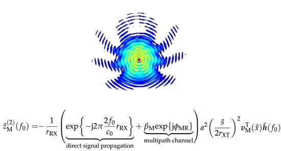
In the last step, the multipath signal propagation from the target to the receive-antenna is included to obtain the receive-signal ${\check{z}}_{\mathrm{M}}^{\left(2\right)}\left(f_0\right)$ as

$$\begin{array}{c}\hfill \begin{array}{c}\hfill {\check{z}}_{\mathrm{M}}^{\left(2\right)}\left(f_0\right)=\frac{1}{r_{\mathrm{RX}}}\left(\underset{\mathrm{direct}\mathrm{signal}\mathrm{propagation}}{\underbrace{\exp \left\{-\mathrm{j}2\pi \frac{2f_0}{c_0}{r}_{\mathrm{RX}}\right\}}}+\underset{\mathrm{multipath}\mathrm{channel}}{\underbrace{{\beta }_{\mathrm{M}}\exp \left\{\mathrm{j}{\varphi }_{\mathrm{MR}}\right\}}}\right){\check{y}}_{\mathrm{M}}^{\left(2\right)}\left(f_0\right).\end{array}\end{array}$$

(31)

Herein, we used again the multipath-to-signal ratio ${\beta }_{\mathrm{M}}$, as we assume that the measurement environment has reciprocal multipath properties. The multipath phase on receive is ${\varphi }_{\mathrm{MR}}$.

4. Simulation Analysis

In this chapter, simulation results are presented. The image dispersion effects due to dynamic nonlinear target transfer functions are introduced using the derived Volterra and multipath model. The signal propagation from the transmit-antenna to the target and from the target to the receive-antenna are already included in the proposed model.

In Section 4.1, we describe simple and easy to implement algorithms for the random generation of dynamic nonlinear transfer functions. These algorithms are divided into two parts. The first part is concerned with dynamic linear impulse responses. In the second part, an algorithm for computing static nonlinear transfer functions is outlined. The transfer functions generated with these two methods are then combined using the pre-computed equations given in Section 3.1.2. We want to mention, that there may exist other, more sophisticated methods for the random generation of nonlinear systems, not only for the discussed examples, but also for more general or complex cases. Here, we restrict ourselves to the straight-forward method discussed in the following.

In Section 4.2, we present an easy method for randomly generating multipath data in conjunction with the model presented in Section 3.2. To this end, we do not want to generate random measurement environments or perform any ray-tracing or electromagnetic full-wave simulations, as it is for example been done in [33]. We define a set of governing rules, that limit the generation of the necessary multipath data. With this method, it is not guaranteed that the multipath data are truly representing physical environments, however, some effects which can be expected to be present in real-world scenarios are captured. This includes the correlation of multipath signals from different measurement channels.

Simulation results illustrating the presented harmonic radar model are shown and discussed in Section 4.3.

4.1. Random Generation of Dynamic Nonlinear System Transfer Functions

To generate random instances of the three example systems discussed in Section 3.1.2, it is necessary to generate random realizations of dynamic linear transfer functions and static nonlinear elements.

Dynamic linear impulse responses—For the generation of a random impulse response $H\left(t\right)$, we establish the following rules:

• $H\left(t\right)=0$ for $t\notin \left(0,T\right)$ : The impulse response has to be causal with finite extend T, as we do not expect any self-oscillatory behavior.
• One global maximum at $T_{\max }$, with local maxima increasing on average towards it for $t=0\dots T_{\max }$ and decreasing on average away from it for $t=T_{\max }\dots T$ : we expect an on average rising and decaying behavior after exciting a target.
• Normalization ${\int }_0^T{\left|H\left(t\right)\right|}^2\mathrm{d}t=1$ : the dynamic linear element should neither amplify nor attenuate an input signal.
• Continuously differentiable: sudden jumps are not expected from physical systems.

Algorithm 1 outlines roughly a scheme to generate random dynamic linear impulse response functions obeying the above defined rules.

Algorithm 1. Random impulse response generator.

Generate two sampled signal containers, one for $t=0\dots T_{\max }$ and one for $t=T_{\max }\dots T$, with an appropriate sampling frequency: Produce samples of a standard normal distribution for each signal bin. Apply a moving average filter until the signal is sufficiently smooth. Span a line from the first sample to the last sample and compute the difference of the two curves. Normalize the new signal samples, such that all samples sum up to one. Compute a new signal container of the same length as the cumulative sum of the old samples. Square the new samples, so that the envelope is positive and without jumps. Rotate the second signal container for $t=T_{\max }\dots T$. Join the two signal containers. Multiply with a sinusoidal signal of the desired center frequency. Normalize, such that the sum of the squared samples is one. Compute Fourier coefficients at the desired frequency values.

Static nonlinear transfer functions—In addition to dynamic linear elements, a random generator for static nonlinear input-output relations $y\left(x\right)$ is required. Again, we set up rules for this:

• The maximum of $|y\left(x\right)|$, within the range of expected input values, should be one: amplification and attenuation is considered separately.
• Continuously differentiable: sudden jumps are not expected.
• Monotonic increasing or decreasing: voltage or current break-ins by increasing the input voltage or current are not expected.
• $y\left(0\right)=0$ : no rest-current (or -voltage).

The outline of a random static nonlinear transfer function generator is given in Algorithm 2.

Algorithm 2. Random static nonlinear transfer function generator.

Produce samples of a standard normal distribution in a one-dimensional container. Apply a moving average filter until the curve is sufficiently smooth. Span a line from the first sample to last sample and compute the difference of the two curves. Shift range of the sample-set to $\left[0,1\right]$. Compute the cumulative summation of the samples. Set the value of the sample associated with $x=0$ to zero, so that $y\left(0\right)=0$ is guaranteed. Scale all samples, so that the maximum of the absolute values is one. Multiply at random with $\pm 1$. Compute all even-order polynomial coefficients up to some desired order.

With Algorithms 1 and 2, it is possible to generate random, but in some sense plausible, dynamic linear and static nonlinear transfer functions. Together with the equations derived in Section 3.1.2, it is possible to compute the relevant symmetrized frequency-domain Volterra kernels.

4.2. Random Generation of Multipath Data

The multipath signals of the total signal chain transmitter—target—receiver are characterized by three parameters: the multipath-to-signal ratio ${\beta }_{\mathrm{M}}$, the transmitter—target multipath phase ${\varphi }_{\mathrm{MT}}$ and the target—receiver multipath phase ${\varphi }_{\mathrm{MR}}$. In the following, a simple random multipath generator is discussed in conjunction with the harmonic radar multipath model (31).

The following rules define random multipath parameters and lead to Algorithm 3.

• Each individual channel (transmitter—target and target—receiver) has an associated set of multipath parameters.
• The multipath data of each channel have to be correlated to other channels based on the spatial separation of the start-point (transmit-antenna or target) and end-point (target or receive-antenna) relative to the signals’ wave-length: in a realistic scenario, it can be expected that small movements of the emitting or receiving element do not lead to significant variations of the multipath channels’ impulse response.
• The time-domain representation of the multipath channels’ impulse response has to decay with increasing travel-time (i.e., signal path length).
• Over all transmitter-, target- and receiver-locations, as well as all desired signal frequencies, the ratio of the multipath amplitude to the direct signals’ amplitude has to be on average ${\beta }_{\mathrm{M}}$.

Algorithm 3. Random multipath data generator.

Generate a sampled impulse response for all signal channels (transmitter—target and target—receiver), using an appropriate sampling frequency, over some desired spatial extend: Draw samples from a uniform distributions within the range $\left[{\rho }_{\mathrm{M},\min },1\right]$, with minimum multipath reflectivity ${\rho }_{\mathrm{M},\min }$, for all signal bins. Divide each random sample by a power of the associated distance (here, we use a power of two). Convert the spatial-domain multipath signal to frequency-domain for all desired signal frequencies. Correlate all frequency-domain multipath data samples according to the spatial separation of the start-point and end-point by a convolution with some kernel function separately for each frequency. Multiply the frequency-domain multipath data of each channel with the associated direct signal path length. Normalize all data points, such that the mean value is ${\beta }_{\mathrm{M}}$.

4.3. Simulation Results and Analysis

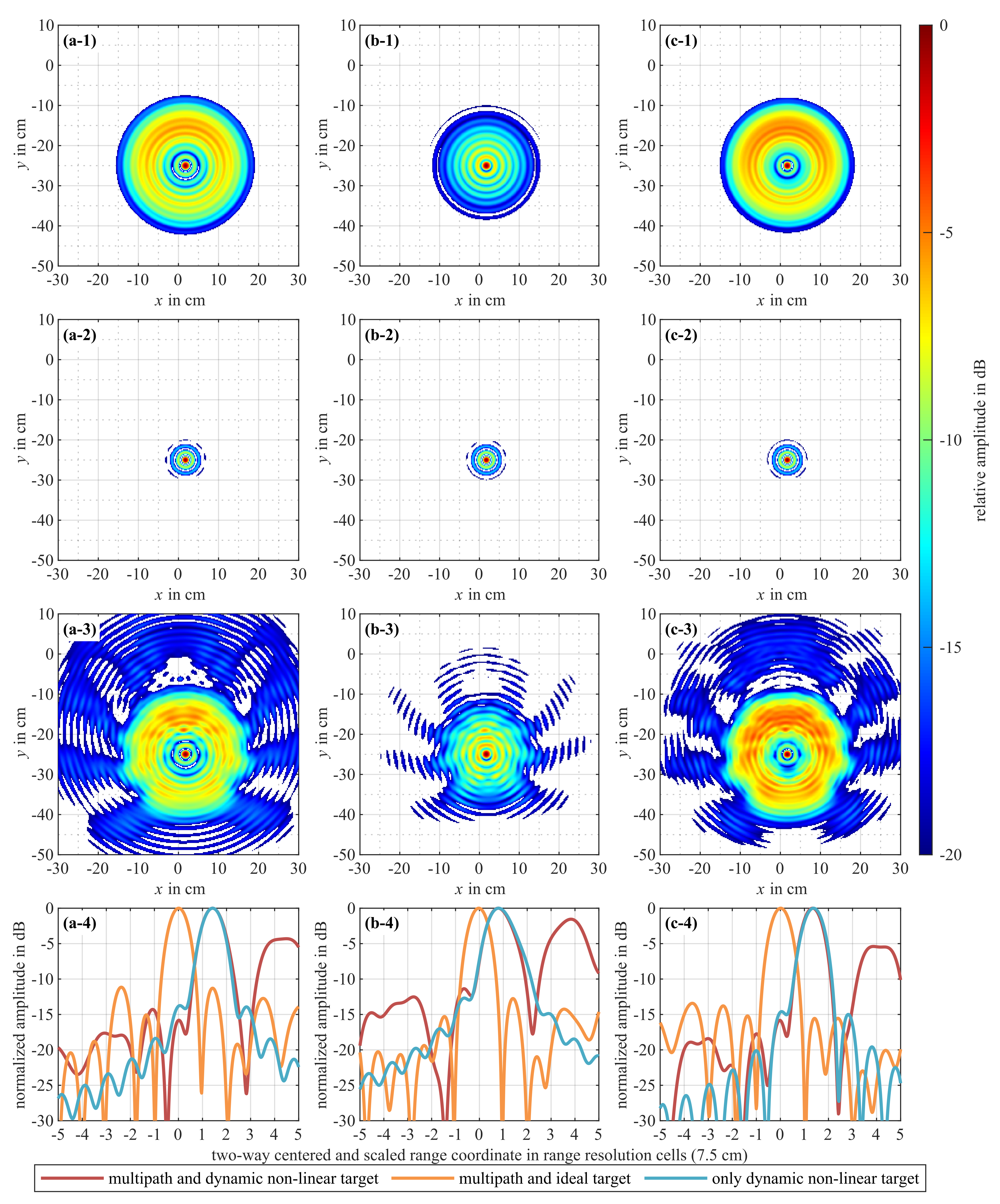
Figure 4 shows a comparison of three randomly generated simulation scenarios (if not mentioned otherwise, all of the explanations and references are with respect to this figure). The simulations are performed with the same geometry and parameter selection as in the measurement results shown in Figure 2 and [9]. For each simulation run, a new random dynamic nonlinear transfer-function is generated by means of frequency-domain Volterra kernels and the algorithms outlined in Section 4.1. Simulation run (a-1,2,3) in Figure 4 is based on the example system model 1 from Section 3.1.2, the simulations (b-1,2,3) and (c-1,2,3) are based on example model 2. In all three instances, a new set of multipath data are used, generated using the method described in Section 4.2. Additional noise is not present in any of the results. The images are generated using the backprojection algorithm. The signal-to-multipath ratio (SMR) is 6 dB (${\beta }_{\mathrm{M}}\approx 0.5$).

The different simulation instances in Figure 4 are indicated by (a-1,2,3), (b-1,2,3) and (c-1,2,3). All images (a,b,c-1,2,3) show maximum projections in the $xy$–plane, with each image being normalized to the respective maximum image value using a logarithmic scaling, normalized to the respective image maxima and a dynamic range of 20 dB. The curves (a,b,c-4) are spatial-domain receive-signals used for the image generation with the backprojection algorithm. The shown range-profiles are examples selected from the same transmit-receive-antenna combination at the same measurement position. The range coordinates measure the two-way distance, centered at the true transmitter—target—receiver signal path length and scaled relative to the resolution of an ideal rectangular band-limited signal with 2 GHz bandwidth. The images are generated with (a,b,c-1) only dynamic nonlinear target functions, (a,b,c-2) multipath signals and ideal target functions and (a,b,c-3) multipath signals and dynamic nonlinear target functions.

Dynamic nonlinear transfer-functions only—In the images (a,b,c-1), we can observe the dispersive influences of the targets transfer-functions on the image quality. The transfer functions are not designed to be dependent on the direction of the impinging signal. Consequently, the image traces in the shown $xy$-plane should appear rotationaly symmetric. The small deviation from this (e.g., (c-1)) is caused by the targets’ off-axial placement. As expected, the images show a significant defocusing and smearing, compared to an ideal image (see (s-1) in Figure 2 for reference). Although in (b-1,2,3) and (c-1,2,3), the same underlying example model is used, their images appear different. Image (b-1) shows a more compact disc compared to (c-1). A reason for this can be obtained by observing (b,c-4; —). In (b-4), the maximum of (—) is close to the true target position (distance less then 1 resolution cell), whereas in (c-4), the maximum of (—) is in a distance of more then one resolution cell, compared to that of the true target position. This effect is caused by the dynamic transfer function, as it adds a time-delay between the reception of the impinging radar signal and the emission of the harmonic signals. This delay, together with the backprojection algorithm, causes a disc-like smearing of the targets’ image trace. The same can be seen in (a-1) and (a-4; —). Increasing the targets’ intrinsic delay should therefore also increase the smearing and disc-like shape in the harmonic radar image.

Multipath signals only—The images (a,b,c-2) do not appear significantly different from an ideal and multipath-free scenario. In addition, no traces of the multipath signals are present in the depicted range of 20 dB. This is different with what is expected in a conventional radar scenario, where clutter and multipath contributions are typically present. In these simulations, only the multipath channels transmitter—environment—target and target—environment—receiver are added to the synthetic data. Multipath data for the channel transmitter—environment—receiver are not included, as this channel is blocked due to the frequency separation between transmission and reception. The influence of the (harmonic) multipath signals is visible in (a,b,c-4; —). Here, the impulse response of the simulated ideal targets has its’ maximum located at the true signal path length, however, with uneven and elevated side-lobes compared to an ideal impulse response (see (b; —) in Figure 3 for reference).

Dynamic nonlinear transfer-functions and multipath signals—Finally, the results of the combined multipath and dynamic nonlinear transfer-function case (a,b,c-3) is analyzed. In general, the image traces keep their overall appearance and characteristics compared to (a,b,c-1). The multipath signals, however, appear to introduce ripples and deviations from the approximate rotational symmetry. The curves (a,b,c-4; —) have their maxima at the same location as the curves without multipath contributions (a,b,c-4; —). This can be expected, because the multipath signals are added to the direct signal and should not introduce additional time delays. The side-lobes are elevated significantly, compared to the other two discussed situations. This indicates that the intermixing of the multipath data with the direct signal through the dynamic nonlinear transfer function introduces an additional deviation to the ideal impulse response.

The general visual appearances of the simulation results (a,b,c-1), and especially (a,b,c-3), are comparable to the measurement result (m-1) shown in Figure 2. The images (a,b,c-3) experience some of the same features, e.g., a smearing of the impulse response, yet keeping the image trace compact and centered around the true target location. The dominant ripples found in the measurement result is also present in the simulations.

5. Conclusions and Outlook

By analyzing measurement data and comparing it to ideal reference simulations, we showed that the observed dispersion effects are caused by the electronic targets. Motivated by these observations and our conclusions, a harmonic radar measurement model incorporating dynamic nonlinear effects, formalized using a Volterra series expansion and a single-frequency excitation, together with a multipath propagation model, was proposed. The derived signal model was tested using simulation studies with a random generation of selected target transfer-functions and multipath signals. The devised random generators are set-up to be computationally inexpensive and simple to implement. They adhere to some predefined rules but are not in every sense physical. Images generated from harmonic radar data using algorithms from conventional radar show some form of defocusing and smearing. These phenomena could be replicated in the discussed simulations using the derived signal model. In addition, the influence of multipath contributions could be observed by simulating different combinations of ideal targets, dispersive targets, multipath environments, and environments without multipath contributions.

The derived signal model reveals differences of harmonic radar to classic radar imaging. In classic radar, the measurement signals can be described as an integration of a function describing the electromagnetic reflectivity of targets and other objects in the measurement scene (see (1)). From this point of view, a target can be described by a single scalar parameter. The spatial reconstruction of this quantity is the goal of radar imaging schemes (e.g., the backprojection algorithm). From the derived model, we conclude that a target described by a dynamic nonlinear transfer-function cannot be described by just one parameter. Instead, it has to be quantified by a collection of frequency-domain symmetrized Volterra kernels, as they result from the derivations shown in here (i.e., (14) and (20)). By computing images using conventional algorithms, it is possible to generate a visual representation of a measurement scene and the targets within, however, the computed quantity has no direct meaning or interpretation. Computing and visualizing the spatial distribution of the Volterra model-parameters might introduce additional problems, as one first needs to be able to compute them using measured data. In addition, a system is described by a series of these coefficients, so a method for accurately visualizing them might become necessary.

The proposed model might also be used to compute the Volterra coefficients as a method for distinguishing or identifying targets. The task of estimating Volterra kernels or coefficients is already known in the engineering literature [34]. With the shown example systems, it might also be possible to pre-compute the Volterra coefficients of some targets or maybe some general classes of targets and use this for target identification or classification purposes.

With the easy to implement random system and multipath generators, it should be possible to test harmonic radar imaging algorithms, evaluate the performance of a possible measurement systems, or to test other algorithms related to harmonic radar applications.

Another possible application of the proposed harmonic radar system model could be to correct known nonlinear transfer functions of cooperative targets (i.e., transponders). With the presented system model and a priori knowledge on the targets’ transfer behavior, a nonlinear inversion procedure, or an impulse response for matched filtering, might be devised.

Future research activities should include testing the theoretical models presented in here with real measured data. This could include a full free-space signal propagation or, as a first step, a closed-loop experiment. These investigations also necessitate an a priori knowledge on the Volterra model parameters, so that the data could be compared to simulations or calculations. A detailed theoretical analysis of the interplay between multipath signals and nonlinear transfer functions is additionally open for investigations.