Joint Use of in-Scene Background Radiance Estimation and Optimal Estimation Methods for Quantifying Methane Emissions Using PRISMA Hyperspectral Satellite Data: Application to the Korpezhe Industrial Site

Abstract

Methane (CH₄) is one of the most contributing anthropogenic greenhouse gases (GHGs) in terms of global warming. Industry is one of the largest anthropogenic sources of methane, which are currently only roughly estimated. New satellite hyperspectral imagers, such as PRISMA, open up daily temporal monitoring of industrial methane sources at a spatial resolution of 30 m. Here, we developed the Characterization of Effluents Leakages in Industrial Environment (CELINE) code to inverse images of the Korpezhe industrial site. In this code, the in-Scene Background Radiance (ISBR) method was combined with a standard Optimal Estimation (OE) approach. The ISBR-OE method avoids the use of a complete and time-consuming radiative transfer model. The ISBR-OEM developed here overcomes the underestimation issues of the linear method (LM) used in the literature for high concentration plumes and controls a posteriori uncertainty. For the Korpezhe site, using the ISBR-OEM instead of the LM -retrieved CH₄ concentration map led to a bias correction on CH₄ mass from 4 to 16% depending on the source strength. The most important CH₄ source has an estimated flow rate ranging from 0.36 ± 0.3 kg·s⁻¹ to 4 ± 1.76 kg·s⁻¹ on nine dates. These local and variable sources contribute to the CH₄ budget and can better constrain climate change models.

1. Introduction

Climate change has become a major preoccupation for society, leading nations to develop common environmental commitments, such as the Paris Agreement (2015). Methane (CH₄) is one of the greenhouse gases (GHGs) chiefly under scrutiny due to its key role in several activity domains. Firstly, CH₄ has significant explosive properties that may result in major infrastructure damage and security issues [1]. CH₄ also has an impact on public health; inhaling high concentrations can lead to respiratory complications. CH₄ also contributes to the formation of tropospheric ozone (O₃), which may have a much higher impact in terms of respiratory and cardiovascular deaths [1,2,3]. Regarding the environment, CH₄ is the second most important anthropogenic GHG in terms of impact on climate and influence on air quality [4]. There is a high concentration of carbon dioxide (CO₂) in the atmosphere, yet CH₄ has a global warming potential approximately 28 times higher on a 100-year scale than that of CO₂ [5,6,7,8,9]. Calculations of CH₄ impact on climate change must consider indirect effects. The oxidation of CH₄ in the presence of nitrogen oxides and sunlight lead to the formation of ozone (O₃) [10,11]. O₃ adds approximately 38% to CH₄ force [2]. Considering all these impacts, the broad social cost of methane resulting from one ton of emission is 50–100 times greater than that of CO₂ [12]. Fortunately, CH₄ has an atmospheric lifetime of about a decade, while the CO₂ lifetime is approximately a century [10,13,14], meaning that reducing emissions will have a quicker impact for mitigating climate change [15,16,17].

Nevertheless, the CH₄ concentration in the atmosphere estimated by ice cores has changed dramatically, from approximately 650 parts per billion (ppb) in the year 1000 to approximately 1700 ppb shortly before the year 2000 [18]. The highest increase in the National Oceanic and Atmospheric Administration’s 37-year record [2] was observed in 2020, with an atmospheric concentration of 1890 ppb. The tripling of CH₄ concentration in a thousand years, as well as the increase in anthropogenic CH₄ compared to natural CH₄, can be explained by human activity. Natural CH₄ sources are wetlands (swamps), termites and oceans, which are relatively time-stable [19]. Anthropogenic sources are distributed in the sectors that followed the industrial revolution: energy (fossil fuel production, etc.), industry, waste treatment (15 to 18% of the anthropogenic balance [20]) and agriculture (rice farming, ruminant farming, etc.) [21]. CH₄ sinks are divided into three categories [22]; the main cause of methane destruction (90% of the sinks [23]) is the oxidation of CH₄ by the hydroxyl (OH) radical in the troposphere, while absorption by soils and oxidation in the stratosphere represent the rest of the CH₄ sinks.

Improved detection and quantification of CH₄ emissions would provide a better constraint for inventories of large-scale CH₄ releases into the atmosphere. Due to CH₄′s explosive properties and the limited accessibility of the source (in the case of major gas leaks), remote sensing is a powerful tool, already validated up to quantification [24]. Satellite sounders, such as TROPOMI (TROPOspheric Monitoring Instrument) [25] on ESA’s Sentinel-5 Precursor satellite, are suitable instruments to study CH₄ emissions on a global scale [9]. However, their kilometric spatial resolution is unsuitable for mapping anthropogenic CH₄ from industry. The dimensions of an industrial plume are typically less than a few kilometers. Detecting industrial plumes is an economic and environmental challenge. Firstly, permanent CH₄ leakage represents a loss of revenue for industries [26]. Secondly, although large emitters dominate the industrial methane emissions budget [27], small sources also contribute to increased CH₄ emissions. Identifying a leak is always a good step towards reducing GHG emissions. Other instruments, called imagers, have a smaller ground pixel size than sounders. The most common are airborne imagers that provide a ground pixel size of approximately a few meters. Airborne imagers, such as AVIRIS-NG (Airborne Visible/Infrared Imaging Spectrometer—Next Generation) [28], can detect and quantify industrial plumes [29]. These imagers can detect small-scale leakages on industrial infrastructure. Once located, dedicated teams can visit the site or a campaign can focus on certain emission points [30]. However, these airborne campaigns are expensive, difficult to perform, and cover only a small portion of the area of interest.

Satellite imagers are a compromise between satellite sounders and airborne imagers. Satellite imagers developed rapidly since 2020; however, it is important to note that two of them are pioneers. Hyperion [31], launched in the late 2000s, detects and quantifies industrial plumes, but the results are established with a super-emitter source [29] and the signal-to-noise ratio (SNR of 20 [32]) of this instrument has limited further studies [33] on weaker sources. Launched in 2016, the GHGSat-D (GreenHouse Gases Satellite) satellite demonstrated the feasibility of detecting CH₄ plumes with a spatial resolution of 50 m, but the data are not freely accessible [34]. The new imaging satellite, PRISMA (PRecursore IperSpettralle della Missione Applicativa) [35], launched in 2019, has a spatial resolution of 30 m and hyperspectral images are available. Recent work has demonstrated the feasibility of using this satellite to quantify methane plumes [36,37,38].

In the literature, two concentration map methods are widely used: the Matched Filtering (Linear Method (LM)) [23,29,39,40,41,42,43,44,45,46] and the Optimal Estimation (OE) method [37,47,48,49,50]. The first method linearizes the mathematical expression of the gas transmission, resulting in an underestimation of the retrieved concentration. In the second method, the standard OE approach [28] requires significant computation time due to the non-linear radiative transfer model computation and the number of parameters to retrieve. In this paper, we propose a new algorithm called ISBR-OE that builds on the LM and OE approaches.

This paper focuses on the Korpezhe oil and gas field, located in a desert area of Turkmenistan. This site was chosen because several significant emission points are present and the background is homogeneous [36]. Based on these data, this paper first highlights the drawbacks of the LM method widely used in the literature, resulting in an underestimation of the retrieved concentration. Then, the second part details a new plume quantification method, called the ISBR-OE method, that builds on the LM and OE approaches in order to obtain results with uncertainty control and reasonable computation time. In order to understand the improvement in the new method, we compared the integrated path concentration estimated from the linear and the new methods using synthetic data and real PRISMA data on different CH₄ plumes. Furthermore, two state-of-the-art flow rate estimation methods and a new method derived from the literature were applied to PRISMA data. We have analyzed CH₄ emission uncertainties derived from integrated path concentration maps for the industrial area studied. All three flow rate estimation methods are based on wind speed. Some approaches try to circumvent using this information by performing large-eddy simulations (LES) to derive the flow rate as a function of the plume shape [51], but these methods are not covered here.

2. Data

2.1. Hyperspectral Images

Launched in March 2019, the PRISMA satellite is equipped with hyperspectral and panchromatic sensors. The Agenzia Spaziale Italiana’s (ASI) policy is to give access to the data to the largest number of users, and it is easy to register on http://prisma-i.it/index.php/en/ (last accessed on 15 June 2021) to obtain data (PRISMA Data Policy Issue 1.0 Date 20 May 2020) which can be provided with various levels of pre-processing (L0, L1, L2B, L2C, L2D) [52]. The hyperspectral camera covers VNIR (visible/near-infrared) and SWIR (short-wave infrared) with respectively 92 and 157 channels [35]. As this paper focuses on CH₄ quantification, only the 113 channels between 1500 and 2500 nm are retained. Indeed, CH₄ has several vibrational absorption bands at wavelengths of approximately 1650 nm and 2350 nm (plus 3400 nm and 7700 nm in mid-wave infrared). The CH₄ monochromatic absorption of the Pacific Northwest National Laboratory (PNNL) database [53], in ppm⁻¹·m⁻¹, is shown in blue in Figure 1. This quasi-monochromatic absorption is then convolved with the PRISMA spectral response function (red line). In this spectral range, the PRISMA satellite has a spectral sampling distance of approximately 9 nm and a spectral resolution (Full Width of Half Maximum) between 9 and 15 nm [54]. The hyperspectral camera’s spatial resolution is approximately 30 m (ground sampling distance) and an image covers an area of 30 km × 30 km.

SNR specifications of PRISMA are described in Labate [35] and listed in

Table 1. Signal-to-noise ratio (SNR) specifications for the PRISMA satellite according to spectral range; requirement specifications come from Labate [35] and the observation-based specifications are estimated in Cogliati [55].

	Spectral Range (nm)	Requirement [35]	Estimation [55]
SNR	1500–1750	≥200	200–400
	1950–2350	≥100	≈100

. Using the Homogeneous Regions Division And Spectral De-Correlation (HRDSDC) method, Cogliati [55] estimated the PRISMA pixel SNR at each wavelength in the spectral dimension (by using the adjacent wavelengths) and scene heterogeneity (by using neighboring pixels in the same homogenous region). The results are provided in Table 1 and comply with the instrument’s specifications.

The images analyzed here focus on an industrial area, with four identified emission points in the west of Turkmenistan, as presented in Figure 2. These sources belong to the Korpezhe oil and gas field (38.52°N, 54.21°E). One of these emission points (D panel in Figure 2) is near a compressor station and has been identified as a strong CH₄ emitter [56]. On this industrial site, we were able to recover eleven images with cloudless sky or with few clouds between 2020/04/19 (YYYY/MM/DD) and 2021/06/22.

Table 2. Wind speed $U_{10}$ in m·s⁻¹ and wind direction expressed in meteorological data frame in degrees, for the images over the Korpezhe site. All images were acquired between 7:14 and 7:24 UTC, and a weighted average was calculated using the two closest ECMWF interpolated values.

Date	Speed (m·s−1)	Direction (°)
2020/04/19	2.6	251
2020/06/22	8.9	281
2020/07/03	5.0	129
2020/07/21	3.3	137
2020/08/07	4.0	331
2020/10/10	7.9	88
2020/11/14	1.2	147
2021/02/09	2.5	67
2021/03/10	1.7	377
2021/04/14	4.3	111
2021/06/22	2.7	148

lists the dates these different images were taken.

2.2. Wind Information

Using discrete (in time or in space) gas concentration measurements, wind speed and direction are required to estimate the gas flow rate (see Section 3.4). In this paper, European Centre for Medium-Range Weather Forecasts (ECMWF) forecasts are used. ECMWF wind data was calculated at 00:00 or 12:00. The forecasts were then used to estimate the 10 m wind components for each hour with a grid of 0.125° × 0.125°, i.e., 13 km × 13 km. The Korpezhe site is located between four ECMWF grid points. The wind direction is expressed in a meteorological data frame. Angles of 0°, 90°, 180° and 270° correspond to wind blowing from the north, east, south and west, respectively. Due to the grid and time of ECMWF data, spatial and temporal interpolations had to be applied. Spatially, the Korpezhe values were obtained by distance-weighted linear interpolation. Temporally, all the images of the analyzed data set were acquired at around 7:20 UTC. The 7:00 and 8:00 UTC values were used to calculate image wind speed by a weighted average. Table 2 lists the wind speed $U_{10}$ and wind direction for the various PRISMA images.

3. Methods

The determination of the total mass of a CH₄ plume and the estimation of the source flow rate require a plume segmentation step followed by a quantification step, which have been implemented in the CELINE code. These two steps are based on the information contained in the radiance spectrum of the hyperspectral image. In the CELINE code, once the pixels affected by CH₄ are identified, the observed radiance is again used to calculate the CH₄ concentration for each plume pixel.

3.1. Direct Model of Radiance as a Function of Plume Concentration

In VNIR-SWIR, the radiance measured by an imaging instrument without any gas plume in the line of sight can be expressed as the sum of three different radiances (in W·m⁻²·sr⁻¹·μm⁻¹⁾ (scheme on Figure A1 in Appendix A). The first radiance, $L_{atm}$, is the atmospheric radiance without any interaction with the ground. The second one, $L_{diff}$, describes the photons that have been scattered towards the sensor after an interaction with the ground. The last one, $L_{dir}$, represents the upwelling radiance directly transmitted from the ground. $L_{diff}$ and $L_{dir}$ are both dependant on the downward solar irradiance and the ground reflectance [57,58]. Therefore, the total measured radiance $L_{no pl}$ (in W·m⁻²·sr⁻¹·μm⁻¹) can be expressed as:

$$L_{no pl}=L_{atm}+L_{diff}+L_{dir}=L_{atm}+\frac{R{E}_o\left({\tau }_{dir}+{\tau }_{diff}\right)}{\pi \left(1-RS\right)},$$

(1)

where $R$ is the ground reflectance, $E_o$ the downward irradiance at ground level (in W·m⁻²·μm⁻¹), ${\tau }_{dir}$ the direct transmission, ${\tau }_{diff}$ the diffusive contribution, and $S$ the spherical albedo of the atmosphere. The total atmospheric transmission ${\tau }_{atm}$ is the sum of ${\tau }_{dir}$ and ${\tau }_{diff}$ and can be expressed as ${\tau }_{atm}=\left(1+\eta \right){\tau }_{dir}$ with $\eta ={\tau }_{diff}/{\tau }_{dir}$.

Scattering effects can be neglected in SWIR. A Radiative Transfer Model (RTM) (COMANCHE [59]) was effectively used to quantify the impact of each term. A sensitivity study was conducted to verify that additional simplifications could be made in the case of the airborne sensor. Firstly, the (1 − RS) term can be approximated by 1 with an error of approximately 0.05% for clear-sky observation conditions. Secondly, the diffusive contribution ${\tau }_{diff}$ is negligible compared to the direct transmission ${\tau }_{dir}$($\eta \ll 1$), which leads to an atmospheric transmission ${\tau }_{atm}={\tau }_{dir}$.

In a near-nadir viewing geometry and taking into consideration the presence of a CH₄ plume in the line of sight, the atmospheric transmission when a plume is present can be expressed as ${\tau }_{dir }^{\prime }={\tau }_{dir}·{\tau }_{CH4}$ with:

$${\tau }_{CH4}=e^{-\rho A \left(1+\frac{1}{\cos \theta }\right)},$$

(2)

where $\rho$ is the integrated line-of-sight concentration (in ppm·m), $A$ the absorption (in ppm⁻¹·m⁻¹) at the instrument wavelengths, and $\theta$ the solar zenith angle. In the following, we replace the term of “integrated line-of-sight concentration” by the term “concentration (in ppm·m)”. Therefore, the radiance in the presence of plume is $L_{pl}$ (see scheme on Figure A1 in Appendix A):

$$L_{pl}=L_{atm}+\frac{R{E}_o{\tau }_{dir}}{\pi }·{\tau }_{CH4}.$$

(3)

Finally, between 1500 and 2500 nm, the atmospheric radiance represents less than 2% of the total radiance in clear-sky conditions. In the following, we assume that ${\tau }_{atm}$ is equivalent to ${\tau }_{dir}$. These reasonable hypotheses result in the following expressions:

$$L_{no pl}=\frac{R{E}_o{\tau }_{dir }}{\pi },$$

(4)

$$L_{pl}=L_{no pl}·{\tau }_{CH4}.$$

(5)

In specific cases where the atmospheric radiance $L_{atm}$ cannot be neglected, a single RTM calculation of $L_{atm}$ for the whole image can be run (or derived from the image outside the plume) and the whole image can be corrected as follow:

$$L_{no pl}^{*}=L_{no pl}-L_{atm} ,$$

(6)

where $L$ is the measured radiance and $L^{*}$ is the corrected radiance. In this case, we assume:

$$L_{pl}^{*}=L_{no pl}^{*}·{\tau }_{CH4}.$$

(7)

3.2. Plume Segmentation

The plume segmentation method consists of calculating a probability score, called the Clutter Matched Filter (CMF) score [43,44,60], used for hyperspectral image analysis. This technique estimates the probability of the presence of a spectral signature $b$ (target gas signature) in the radiance spectrum $L$ for each pixel, considering the covariance of the image background. Assuming that the background spectrum follows a normal distribution with a mean background spectrum $L_{bkg}$ and a covariance matrix $C$, the CMF method tests the most likely hypothesis between $H_0$ where the target gas is absent (no-plume pixel), and $H_1$ where the gas is present, e.g.,

$$H_{0 }:L \approx N\left(L_{bkg},C\right),\hspace{1em}\hspace{1em}{H}_{1 }:L \approx N\left(L_{bkg}+\alpha b,C\right).$$

(8)

The CMF method estimates the value of the parameter $\alpha$ that is quantifying the strength of the gas signature $b$ in the background signal. The closer it is to the $b$-signal gas signature in the image, the greater the value of $\alpha$. An improvement of the CMF method, quickly introduced by Funk [43] and widely applied in the literature, uses image clustering as pre-processing [23,29,39,40,41,42]. Once the image is divided into $K$ clusters (or classes thanks to K-means algorithm), an average background spectrum and a covariance matrix are calculated for each class. This improvement is called the Cluster-Tuned Matched Filter or CTMF method. The expression of the CTMF score ${\alpha }_j$ for pixel $\left(x,y\right)$ among $z_j$ pixels of the class $j$ is:

$${\alpha }_j\left(x,y\right)=q_j·\left(L{\left(x,y\right)}_j-L_{mean,j}\right),$$

(9)

where the optimal filter $q_j$ of the class $j$ is expressed as [43]:

$$q_j=\frac{{b_j}^T{C}_j^{-1}}{\sqrt{{b_j}^T{C}_{\mathrm{j}}^{-1}{b}_j}} ,$$

(10)

and $L_{mean,j}$ is the mean radiance of the class $j$ and $C_j$ the class covariance matrix [61], such that:

$$L_{mean,j}=\frac{1}{Z_j}{{\displaystyle \sum }}_{iϵj}L\left(x_i,y_i\right) \mathrm{and} C_j={{\displaystyle \sum }}_{iϵj}\left(L\left(x_i,y_i\right)-L_{mean,j}\right){\left(L\left(x_i,y_i\right)-L_{mean,j}\right)}^T.$$

(11)

The gas signature $b$ must be homogeneous to $\left(L\left(x,y\right)-L_{mean,j}\right)$ to which the optimal filter $q_j$ is applied (Equation (9)). The observed radiance for plume pixels corresponds to the $L_{pl}$ of the direct model (Equation (5)). An important hypothesis is the approximation of the no-plume radiance of Equation (4) by $L_{mean,j}$ to determine the expression of $b$ (right term of the following equation):

$$L{\left(x,y\right)}_j-L_{mean,j}=\left({\tau }_{CH4}-1\right)L_{mean,j}=b_j.$$

(12)

The CTMF score results in a detection map of pixels impacted by CH₄. A threshold value of the score and morphological transformations are applied to isolate the CH₄ plume in the hyperspectral image (see Discussion in Section 5.3).

3.3. Quantification Step: Concentration

Once the mask of the plume pixels has been established, the CELINE code starts the quantification of the CH₄ plume in terms of concentration.

3.3.1. Linear Method (LM)

One of the most widely used methods for quantifying the plume concentration is based on Equation (12). The non-linearity of the problem is the main difficulty of the inversion. This method, which we call the linear method, uses a linearized expression for the methane transmission. Indeed, in the first-order Taylor series approximation, we can express ${\tau }_{CH4}$ as:

$${\tau }_{CH4}=e^{-\rho A\left(1+\frac{1}{\cos \theta }\right)}\approx 1-\rho A\left(1+\frac{1}{\cos \theta }\right).$$

(13)

In this case, the Equation (12) becomes:

$$L{\left(x,y\right)}_j-L_{mean,j}=-\rho A\left(1+\frac{1}{\cos \theta }\right)L_{mean,j}=\rho d_j.$$

(14)

A linear inversion gives the concentration directly as:

$${\rho }_{LM}=\frac{\left(L{\left(x,y\right)}_j-L_{mean,j}\right)C_j^{-1}{d_j}^T}{d_j{C}_j^{-1}{d_j}^T}.$$

(15)

The LM is often presented as a method derived from the CTMF score (a derivative of the Matched Filter) [27,33,46,62]. Indeed, it is possible to express the concentration as the CTMF score divided by the optimal filter $q_j$ applied to the theoretical signal $b_j$. When the hypothesis of low plume concentrations is no longer valid, an underestimation of the concentrations is observed as discussed below.

3.3.2. Optimal Estimation (OE) Method

To retrieve plume concentrations, OE is also commonly used in the literature [47,48,49]. The aim of this method was initially to retrieve the atmospheric composition by minimizing a cost function [24]. The standard OE approach uses iterative RTM computations to find the smallest difference between observed and modeled radiances [48]. In this approach, the state vector $\mathit{x}$ contains all parameters that contribute to the radiance collected by the instrument, in particular the atmospheric composition and the ground reflectance. The inversion requires a model $\mathit{F}\left(\mathit{x}\right)$ to fit the observed radiance $\mathit{y}$ as:

$$\mathit{y}=\mathit{F}\left(\mathit{x}\right)+\mathbf{ϵ},$$

(16)

where $\mathbf{ϵ}$ is the sum of instrument and model errors. As the forward model is non-linear, the state vector is obtained iteratively. The Gauss–Newton solution is presented in Rodgers [24] as:

$${\mathit{x}}_{i+1}={\mathit{x}}_a+{\left({\mathit{K}}_i{\mathit{S}}^{-1}{\mathit{K}}_i^T+{\mathit{S}}_a^{-1}\right)}^{-1}{\mathit{K}}_i{\mathit{S}}^{-1}\left({\left(\mathit{y}-\mathit{F}({\mathit{x}}_i)\right)}^T+{\mathit{K}}_i^T\left({\mathit{x}}_i-{\mathit{x}}_a\right)\right).$$

(17)

In this equation, ${\mathit{x}}_i$ is the state vector at the iteration $i$, ${\mathit{x}}_a$ the prior estimation of the state vector, and ${\mathit{S}}_a$ the prior error covariance matrix. $\mathit{S}$ is the covariance matrix of the image’s pixels and ${\mathit{K}}_i=\frac{\partial \mathit{F}}{\partial \mathit{x}}{|}_{x=x_i}$ the Jacobian matrix calculated for each iteration. This iterative inversion is applied to each plume pixel. OE inversion provides accurate results and has been used, for example, to determine the potential of next-generation imagers, such as PRISMA, to detect and quantify CH₄ point sources [37]. In this latter reference, the authors use the Iterative Maximum a Posterior Differential Optical Absorption Spectroscopy (IMAP-DOAS) algorithm [63,64] and a polynomial decomposition of the surface reflectance to characterize the algorithm’s response to the surface type (grass, bright, dark or urban). In this case, the forward model is expressed as:

$$F^h\left({\mathit{x}}_{\mathit{i}}\right)=I_0\left(\lambda \right)\exp (-A{{\displaystyle \sum }}_{n=1}^3{s}_n{{\displaystyle \sum }}_{l=1}^{72}{\tau }_{n,l}){{\displaystyle \sum }}_{k=0}^K{a}_k{P}_k\left(\lambda \right),$$

(18)

where $I_0$ is the incident top-of-atmosphere (TOA) solar intensity, $A$ the geometric air mass factor, ${\tau }_{n,l}$ the default optical depth from the US Standard Atmosphere (from MODTRAN [65]) for trace gas element $n=\left[1;3\right]$ of the state vector at vertical level $l=\left[1;72\right]$, $s_n$ the scaling factor to that default optical depth optimized retrieval, $P_k$ the k^th Legendre polynomial, and $a_k$ the coefficients optimized in the retrieval. However, iterative RTM computations for each pixel can be time-consuming and require good knowledge of non-retrieved parameters. In this paper, we combine the standard OE approach with a method to reconstruct the background (see below).

3.3.3. in-Scene Background Radiance (ISBR)—Optimal Estimation Method (OEM)

The method used in this paper is based on OE and the ISBR method developed for this study which can be referred to as ISBR-OEM. Nevertheless, the ISBR method can be applied to other algorithms, such as LM, to result in ISBR-LM.

The ISBR method is based on three assumptions. First, the radiance observed by the sensor in the presence of the plume can be written as $L_{obs}=L_{bkg}·{\tau }_{CH4}$ (Equations (4) and (5)). Second, the background radiance $L_{bkg}$ can be rebuilt from the spectra contained in the image itself without RTM. Finally, the reconstruction of background radiance reduces the number of parameters to be retrieved to one, i.e., the state vector $\mathit{x}$ of the standard OE approach only comprises the plume concentration $\rho$. The inverse problem’s (Equation (16)) solution thus becomes:

$${\rho }_{i+1}={\rho }_a+{\left({\mathit{K}}_i{\mathit{S}}^{-1}{\mathit{K}}_i^T+{\mathit{S}}_a^{-1}\right)}^{-1}{\mathit{K}}_i{\mathit{S}}^{-1}\left({\left(\mathit{y}-{\mathit{F}}_{\mathit{I}\mathit{S}\mathit{B}\mathit{R}}({\mathbf{\rho }}_i)\right)}^T+{\mathit{K}}_i^T\left({\mathbf{\rho }}_i-{\mathbf{\rho }}_a\right)\right).$$

(19)

The main advantage of ISBR-OEM is that, unlike in previous papers, an RTM is not required, avoiding a complex and time-consuming step. The forward model ${\mathit{F}}_{\mathit{I}\mathit{S}\mathit{B}\mathit{R}}\left(\rho \right)$ is written as:

$${\mathit{F}}_{\mathit{I}\mathit{S}\mathit{B}\mathit{R}}\left(\rho \right)={\mathit{L}}_{\mathit{b}\mathit{k}\mathit{g}}·{\mathbf{\tau }}_{\mathit{C}\mathit{H}\mathbf{4}}\left(\rho \right).$$

(20)

For an in-plume pixel, background radiance cannot be obtained directly because this would require an image taken just before the start of the emission and temporally very close to the time of the plume image studied. Therefore, the ISBR method’s background estimation steps are: (i) image classification using CH₄ non-absorbing channels, (ii) for each in-plume pixel, a set of no-plume pixels spectrally similar (corresponding to the same class as the target in-plume pixel) in the area surrounding the plume are selected; (iii) root mean square error (RMSE) is used to identify the “selected” pixel; (iv) in-plume pixel background radiance for the CH₄ absorbing channels is assumed to be the corresponding radiance of the “selected” pixel.

The a priori concentration ${\mathit{x}}_a={\rho }_{LM}$ is derived from the linear method even if the a priori has to be independent of the observation in the standard OE approach. To limit the share of observation in a priori knowledge, we used a prior error of 100% of the a priori concentration in the prior error covariance $S_{LM}$. The a priori concentration is also the initial state ${\mathit{x}}_0$. The ISBR-OEM’s solution is then expressed as:

$${\rho }_{i+1}={\rho }_{LM}+\widehat{{\mathit{S}}_{\mathbf{\rho }}^{-\mathbf{1}}}{\mathit{K}}_i{\mathit{S}}^{-1}\left({\left(\mathit{y}-{\mathit{L}}_{\mathit{b}\mathit{k}\mathit{g}}·{\mathbf{\tau }}_{\mathit{C}\mathit{H}\mathbf{4}}\left({\rho }_i\right)\right)}^T+{\mathit{K}}_i^T\left({\mathbf{\rho }}_i-{\mathbf{\rho }}_{LM}\right)\right).$$

(21)

The covariance matrix $\mathit{S}$ is calculated for each class without using the pixels identified as belonging to the plume. The a posteriori uncertainty of the retrieved concentration is commonly defined as $\widehat{{\mathit{S}}_{\mathbf{\rho }}^{-\mathbf{1}}}={\mathit{K}}_i{\mathit{S}}^{-1}{\mathit{K}}_i^T+S_{LM}^{-1}$ [47,48]. This a posteriori covariance matrix is providing a robust confidence interval for the concentration (for each plume pixel), from which a reliable uncertainty on the flow rate is estimated.

3.4. Quantification Step: Flow Rate

Once the wind information associated with the image is available, an estimation of the source flow rate is calculated by the CELINE code and we compare three methods of flow rate estimation.

3.4.1. Integrated Mass Enhancement (IME) Method

The IME method is commonly used to calculate flow rates from a gas concentration map [27,34,36,51], and it does not use wind direction. The IME method relates the flow rate $Q_{IME}$ to the plume’s total mass IME (in g), the wind speed $U$ (in m·s⁻¹) and the characteristic size of the plume $L$ (in m) as:

$$Q_{IME}=\frac{U}{L}\left(\mathsf{\Sigma }{C}_{plume}·A_{plume}\right)=\frac{U}{L}·IME=F_{IME}·U,$$

(22)

where $\mathsf{\Sigma }{C}_{plume}$ is the concentration of the plume-pixel (in g), and $A_{plume}$ the surface of the plume (in m²). The characteristic size of the plume $L$ is defined as the square root of the plume surface area [37]. $F_{IME}$ is the IME factor (in g·m⁻¹) similar to a mass per unit length of the following methods.

3.4.2. Cross-Sectional Flux (CSF) Method

The CSF method was developed to be efficient computationally and conceptually simple to estimate a source’s ozone and aerosol flow rates [66]. This method is commonly used in the literature to estimate gas flow rates [7,67,68,69,70]. The product of the mass per unit length $m_{ul CSF}$ (or line density) by the wind speed $U$ results in a flow rate value $q$ at each distance $d$ of the source as followed:

$$q\left(d\right)=m_{ul CSF}\left(d\right)·U\left(d\right).$$

(23)

To obtain the source’s flow rate $Q$ (in g·s⁻¹), an average of $q\left(d\right)$ is calculated over a distance range from the source. In our study, the wind speed grid is larger than the image dimension. The wind speed $U$ (in m·s⁻¹) is assumed to be constant in the entire image. Averaging $q\left(d\right)$ is the same as averaging $m_{ul CSF}\left(d\right)$ (in g·m⁻¹). Then, $Q$ is defined as:

$$Q_{CSF}=<m_{ul CSF}\left(d\right){>}_D· U,$$

(24)

where $< {>}_D$ is the mean operator between the source point and the distance D.

Estimating the principal wind direction is a critical point of the CSF method. The mass per unit length $m_{ul CSF}\left(d\right)$ is effectively obtained by summing the mass present on a slice perpendicular to the wind direction.

3.4.3. Rings Decomposition of Mass (RDM) Method

The local wind direction in the case of industrial plumes is not easy to estimate. Turbulence effects or the presence of obstacles (buildings, etc.) create variations in wind direction over very short timescales. In order to avoid this variability, a method independent of wind direction was developed during this work and based on a flow rate retrieval algorithm developed by SPASCIA society (see authors affiliation). After selecting the source pixel, the RDM method calculates the sum of the mass inside successive concentric rings (with the source point as centre) to obtain the mass per unit length $m_{ul RDM}\left(d\right)$ as a function of the distance to the source. As previously, after spatial averaging of $m_{ul RDM}\left(d\right),$ a multiplication by the wind speed leads to the RDM flow rate $Q_{RDM}$ as:

$$Q_{RDM}=<m_{ul RDM}\left(d\right){>}_D· U.$$

(25)

The radius of the rings is an input parameter. Choosing a small step (30 m or 1 pixel between successive rings) brings this method closer to the CSF method, while a step size covering the entire plume results in a calculation comparable to the IME method. The step has an impact on the uncertainty associated with the measurement.

4. Results

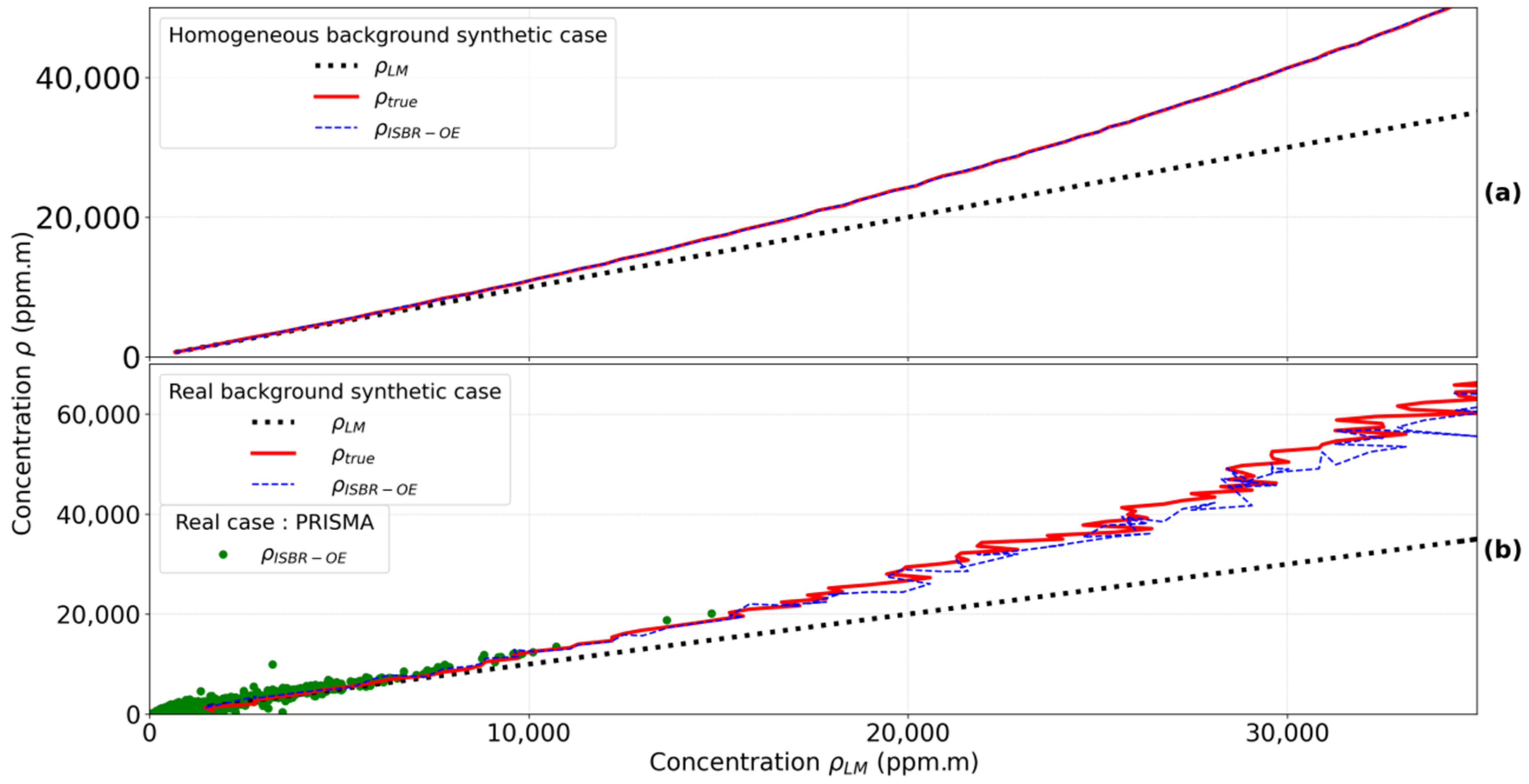
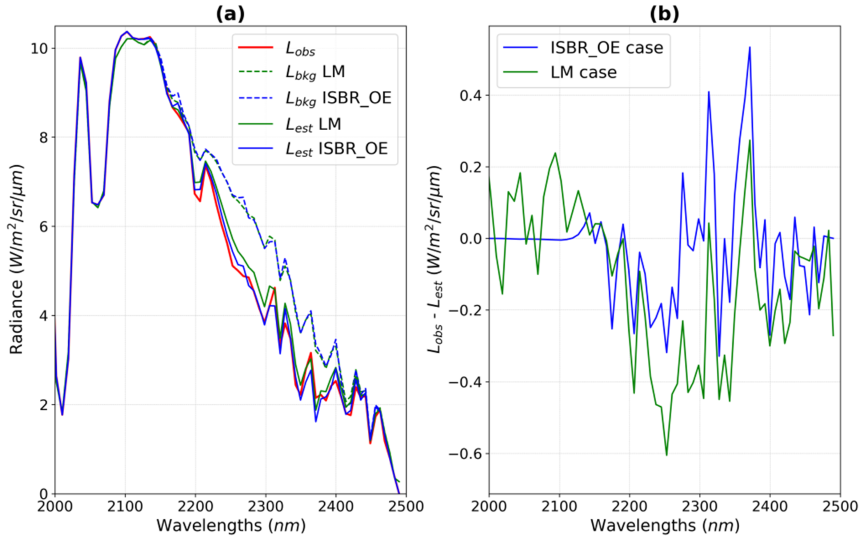
4.1. LM versus ISBR-OEM

LM is the most common plume concentration quantification method. However, transmission linearization results in an underestimation of the retrieved concentration, especially for high concentration values. In order to illustrate this effect, we used a reflectance image using a land surface reflectance database and standard atmospheric parameters to create a radiance image (using the formula in Section 3.1) with a synthetic plume of known concentration (see Figure A3 in Appendix C) added to an atmospheric signal. The background reference signal corresponds to a standard atmosphere of MODTRAN code (mid-latitude summer atmospheric profiles and concentrations) [65]. This image is then processed by LM and ISBR-OEM. The results are plotted in Figure 3; the true and retrieved ISBR-OEM concentrations are shown as a function of the retrieved LM concentration. This particular graph compares the real case (PRISMA) and the synthetic case. The reflectance used in Figure 3a is based on the reflectance spectrum of a brick material (ECOSTRESS JPL Spectral Library at https://speclib.jpl.nasa.gov/ [71,72], last accessed on 25 January 2021) with synthetic noise according to PRISMA SNR (SNR of 150 at 2300 nm), while Figure 3b is based on a real reflectance map from a SWIR image over an industrial site [73]. The synthetic concentration curves (in red) are above the first bisector, meaning an underestimation of the concentration obtained with the LM as expected [73]. The higher the synthetic concentration, the higher the underestimation. Concerning ISBR-OEM (blue dashed line), the synthetic concentration is perfectly retrieved in the simple reflectance map case, and retrieval is fairly similar to the simulation for the real reflectance map despite scene heterogeneity and the interclass variability.

In the test cases, the ISBR-OEM-retrieved concentration is equal to the input synthetic concentration, and the gap between ISBR-OEM and LM increases with concentration. The test cases give confidence in the results for the real case; the gap between ISBR-OEM and LM concentrations is almost the same with a real PRISMA image (green dots in Figure 3b) corresponding to the 2020/07/21 plume. As before, LM concentrations are lower than ISBR-OEM concentrations with the PRISMA image.

Figure 4 corresponds to a spatial comparison of the plume concentration maps for the 2020/07/21 PRISMA image using LM (Figure 4a) and ISBR-OEM (Figure 4b). The absolute difference between ISBR-OEM and LM concentrations is shown in Figure 4c. The difference between the two methods is less significant in the low concentration parts than in the more concentrated parts of the plume. Nevertheless, the spatial smoothness of the plume with LM seems more realistic than with ISBR-OEM. This is mainly because in case of non-convergence of the OE, the concentration values are set to 0. The highest concentration pixel has a mass difference of 30%, which can be significant in terms of the estimated total mass emitted by the source and thus the flow rate. LM can be used up to a maximum concentration of approximately 6000 ppm·m to be less sensitive to underestimation (and for a signal sufficiently higher than the SNR). The analysis in terms of total mass and flow bias is presented for two plumes in Section 4.3.

As the concentration map of the real plume is unknown, comparison between real and retrieved concentrations must be replaced by a comparative study of the measured and estimated radiances. Figure 5a represents (in red) the instrument-measured radiance for the highest concentration pixels near the source (approximately 20,000 ppm·m for the 2020/07/21 plume) for the wavelengths zoomed from 2000 to 2500 nm. The other colors portray LM and ISBR-OEM (green and blue, respectively) results, while other lines represent different types of radiance: the dashed lines represent the estimated background radiances $L_{bkg}$ used in the method, and the solid lines represent the instrument-estimated radiances calculated using the retrieved concentration value. The $L_{bkg LM}$, i.e., the mean radiance of the class, is close but not equal to the $L_{bkg \mathrm{ISBR}-\mathrm{OEM}}$ obtained by the ISBR method. When these spectra are used to estimate the radiance with the associated retrieved concentration (respectively 16,000 ppm·m for LM and 20,000 ppm·m for ISBR-OEM), the ISBR-OEM spectrum is closer to the measured radiance than the LM spectrum. The residuals of the two methods are shown in Figure 5b. The residual’s associated norm is 0.32 W·m⁻²·sr⁻¹·µm⁻¹ for the ISBR-OEM case compared to 0.39 W·m⁻²·sr⁻¹·µm⁻¹ for the LM case. The ISBR-OEM residual’s associated norm is closer to the expected noise value in this spectral range for PRISMA data. This noise is estimated to be around 0.25 in the CH₄ absorption bands. ISBR-OEM avoids any linearization of the gas transmission. Using an estimation of the background radiance that varies for each pixel reduces residuals. The CH₄ signature has been largely suppressed in the residuals.

Furthermore, ISBR-OEM benefits verification values from the standard OE approach, such as the degree of freedom or the ${\chi }^2$ value. Examples are shown in Figure 6 for the 2020/07/21 PRISMA image. In the case of a state vector with one parameter, the concentration in this study, the degree of freedom can be interpreted as the share of the retrieved concentration coming from the measurement and independent to a priori information. This parameter must tend towards unity to ensure that the inversion is not over constrained by the a priori. Figure 6a shows a degree of freedom of approximately 0.99 in the most concentrated area and higher than 0.5 in the rest of the plume. The ${\chi }^2$ value corresponds to the normalized mean square deviation between the observed and the modelled radiances for each wavelength. A ${\chi }^2$ value close to unity means a correct estimation of retrieval uncertainty. Figure 6b shows a few pixels between 0.5 and 1, which can be interpreted as a small overcorrection, while a few others near the plume head are insufficiently corrected (${\chi }^2>1)$. Nevertheless, the results remain close to unity which gives confidence to inversion results. In addition, the standard OE approach estimates a posteriori uncertainty [47]. For each plume pixel, retrieved concentration uncertainty is obtained in ppm·m, which can provide an estimation of the accessible concentration range. The a posteriori uncertainty for the plume in Figure 6 has an average value of approximately 350 ppm·m.

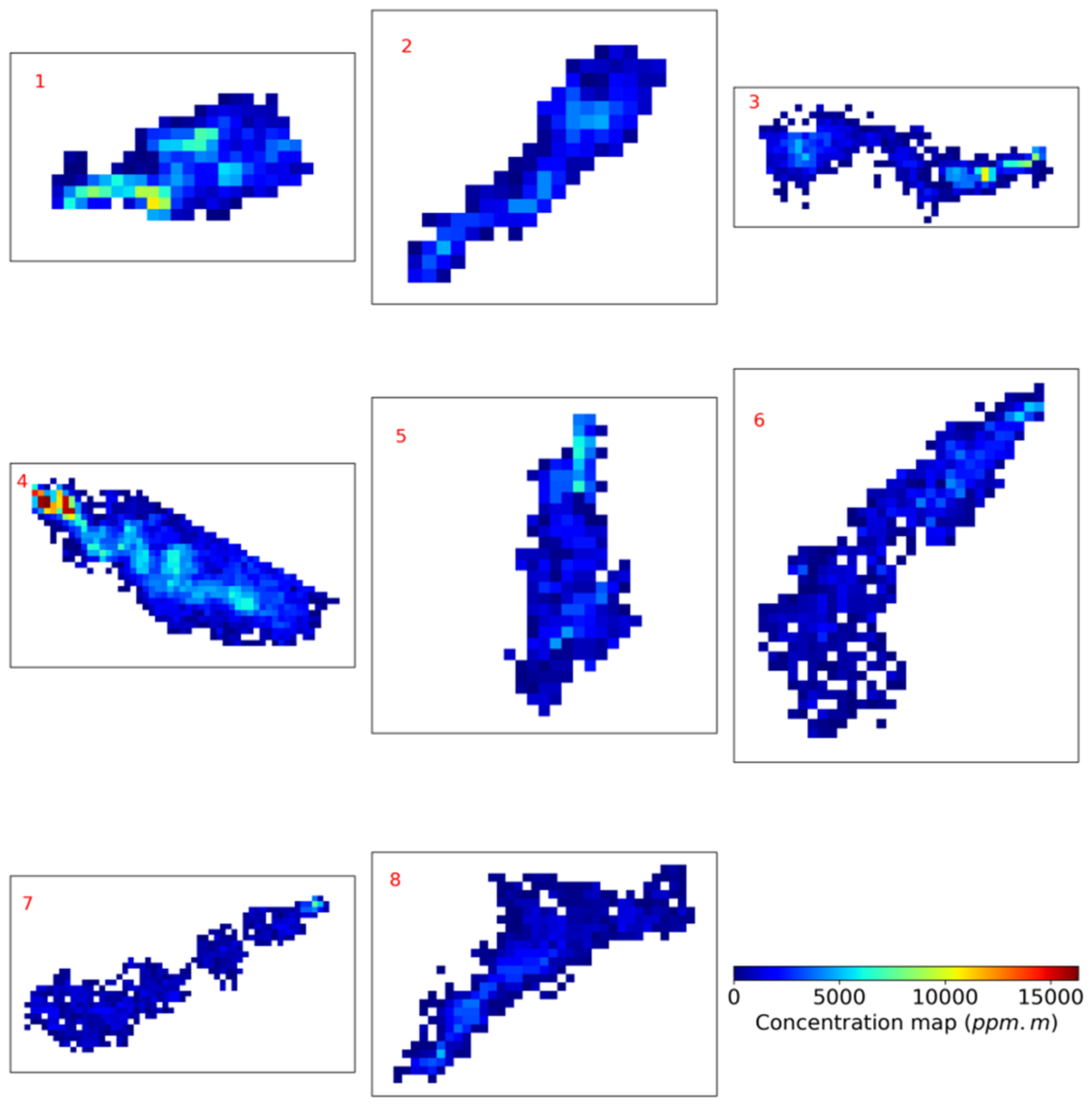
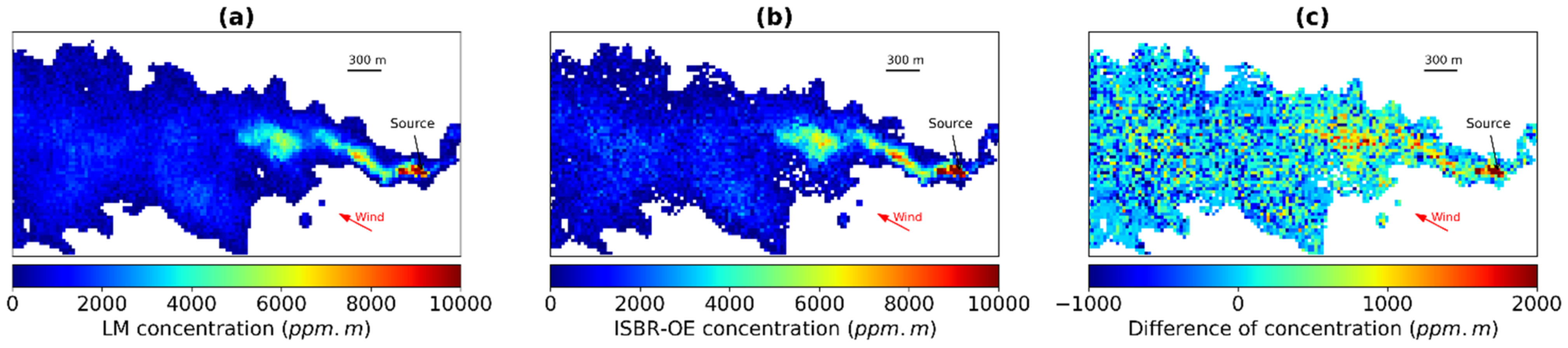
4.2. Overview of the Concentration Map

Here, only ISBR-OEM results are provided and discussed. Of the eleven images in the dataset, nine show a plume corresponding to source A (Figure 2), while the plume corresponding to source D is only seen in two images. Source B and C plumes are seen only once.

Independently of the sources and dates, thirteen plumes were detected. Focusing on the plume head, the plume from source A on the 2020/07/21 image, used as an illustration in the previous sections, shows the highest concentration with a maximum pixel of approximately 20,000 ppm·m. The maximum concentration values for each detected plume are listed in

Table 3. Maximum concentration (in ppm·m) for each plume detected as a function of the source. Seven of the thirteen plumes have a maximum concentration above 10,000 pmm·m.

Date	Source	Concentration Max (ppm·m)
2020/04/19	A	10,700
2020/06/22	A	4790
2020/06/22	D	4920
2020/07/03	A	10,520
2020/07/21	A	20,010
2020/08/07	A	16,300
2020/08/07	C	6790
2020/10/10	D	14,320
2020/11/14	B	11,940
2021/02/09	A	6570
2021/03/10	A	5470
2021/04/14	A	7470
2021/06/22	A	15,390

. To summarize, three plumes are marked for source A. Sources B and D each have one plume that appears significant, while the source C plume is less intense.

For illustration, Figure 7 shows plume concentrations maps on the four sources. Plumes not presented in Figure 4b and Figure 7 are shown in Figure A2 of Appendix B. A mask delimiting the plume contours was applied. These masks including the whole plume are called “full” masks. It is possible to see on this figure, especially on the plume of source D, estimation errors due to the terrain.

Indeed, these sources are distributed in a desert with roads and bright sand banks. The dispersion of a gas by wind advection and turbulence leads to a progressive decrease of the concentration as a function of the distance from the source. However, we observe a small local disturbance in this variation when the plume is covering road pixels. This disturbance is larger over a bright sand bank corresponding to high CTMF values (false alarms), probably due to the intra-class variability or “confuser” pixels that lead to a poor reconstruction of the background signal (see Discussion Section 5.4). The case of the 2020/10/10 image corresponding to source D illustrates the consequence of the presence of bright sand banks. The rectangle and the ellipse on the D source plume correspond to overestimated concentration areas and are linked to the presence of bright sand banks. If not considered, these artefacts have an impact on the estimation of the average mass and consequently on the estimation of the flow rate.

4.3. Mass per Unit Length or Wind Normalized Flow Rate Analysis

This section presents results for the flow rate quantification methods presented in Section 3 in terms of mean mass per unit length $<m_{ul}>$ and $F_{IME}$. The mean mass per unit length corresponds to the flow rate normalized by the wind speed (Section 2.2). The results are detailed in the case of ISBR-OEM retrieval and then compared to the LM retrieval. To analyze these methods, the most stable plumes were focused on. A stable plume must be as close as possible to a Gaussian plume, which settles in a constant emission regime and for which the mass spatial distribution follows a Gaussian model [74,75]. Thus, this analysis is based on two plumes of source A from the 2020/07/21 and 2021/06/22 images, shown respectively in Figure 4 and Figure 7, and respectively referred to as P1 and P2 below.

The CSF and RDM methods are first considered. Figure 8 shows the spatial evolution of the mass per unit length of P1 as a function of the distance $d$ to the source (located at $d=0$) for the CSF and RDM methods shown in a bold line. The mass per unit length $m_{ul}\left(d\right)$ is obtained by summing the mass present on a slice of the plume (perpendicular to the wind direction for CSF and in the ring for RDM). The areas in blue (CSF method) and with orange dots (RDM method) correspond to the sum of a posteriori uncertainties from the OE approach. These uncertainties do not include the loss mass due to the detection threshold, which increases with the distance to the source. The CSF and RDM methods provide equivalent results as shown in Figure 8, but the RDM method does not use the wind direction estimation.

The mean of the mass per unit length is calculated from these curves, and in order to minimize the errors due to the ground artefacts presented in Section 4.2, two masks have been established. The “small” mask covers the immediate environment of the source with an extension of 1400 m (excluding the road pixels or bright sand banks) and the “full” mask includes most of the concentration (see Figure 7). These masks have a direct impact on the mean of the mass per unit length and the associated uncertainty. The $<m_{ul}>$ uncertainty is lower with the small mask than with the full mask. Indeed, the associated uncertainty varies from 21.8 (23.4) g·m⁻¹ to 36.8 (39.9) g·m⁻¹ for the CSF (RDM) method from the small to the full mask, respectively. For the IME method, the uncertainty varies from 181.5 to 455.2 g·m⁻¹ with the small and the full mask, respectively. As shown in

Table 4. Estimation of the wind normalized source flow rate corresponding to plumes P1 and P2 using ISBR-OEM retrieved concentration and CSF, RDM or IME flow rate estimation methods.

Plume	Mask	$<{\mathit{m}}_{\mathit{u}\mathit{l} \mathit{C}\mathit{S}\mathit{F}}>$ (g·m−1)	$<{\mathit{m}}_{\mathit{u}\mathit{l} \mathit{R}\mathit{D}\mathit{M}}>$ (g·m−1)	${\mathit{F}}_{\mathit{I}\mathit{M}\mathit{E}}$ (g·m−1)	Total Mass (kg)	Number of Plume Pixels
P1	Small	617.0 ± 21.8	635.5 ± 23.4	1443.0 ± 181.5	1258.4 ± 158.3	845
P1	Full	727.0 ± 36.8	746.8 ± 39.9	1572.7 ± 455.2	3271.3 ± 946.7	4807
P2	Small	533.1 ± 16.1	558.4 ± 17.2	1222.2 ± 114.1	720.4 ± 67.3	386
P2	Full	548.4 ± 27.1	552.9 ± 28.4	1146.2 ± 324.6	2106.6 ± 596.5	3753

, $F_{IME}$ values are more than the double of CSF and RDM values due to the fact that the effective wind values to be considered are higher for the last two methods than for IME (see Section 5). The other cases are listed in

Table A1. Estimation of the wind normalized source flow rate in cases where the small mask is used.

Date	Source	$<{\mathit{m}}_{\mathit{u}\mathit{l} \mathit{C}\mathit{S}\mathit{F}}>$ (g·m−1)	$<{\mathit{m}}_{\mathit{u}\mathit{l} \mathit{R}\mathit{D}\mathit{M}}>$ (g·m−1)	${\mathit{F}}_{\mathit{I}\mathit{M}\mathit{E}}$ (g·m−1)	Masse Max (kg)	Total Mass (kg)	Number of Plume Pixels
2020/04/19	A	339.6 ± 16.4	339.9 ± 17.1	629.7 ± 81.5	6.33	224.3 ± 29.0	141
2020/06/22	A	140.7 ± 16.8	148.1 ± 19.0	338.9 ± 80.1	2.83	102.2 ± 24.2	101
2020/06/22	D	131.7 ± 16.1	128.4 ± 17.1	298.6 ± 95.2	2.91	154.1 ± 49.2	296
2020/07/03	A	204.6 ± 19.4	232.0 ± 23.9	392.0 ± 75.2	6.22	104.5 ± 20.0	79
2020/07/21	A	617.0 ± 21.8	635.5 ± 23.4	1443.0 ± 181.5	11.91	1258.4 ± 158.3	845
2020/08/07	A	653.5 ± 29.6	666.1 ± 31.8	1357.0 ± 200.9	9.64	1039.5 ± 153.9	652
2020/08/07	C	182.5 ± 22.4	183.0 ± 25.4	297.8 ± 82.2	4.01	76.8 ± 21.2	74
2020/10/10	D	413.2 ± 17.8	458.0 ± 20.4	666.4 ± 85.1	8.46	247.3 ± 31.6	153
2020/11/14	B	732.6 ± 39.3	781.4 ± 42.3	1185.5 ± 227.0	7.06	703.2 ± 134.6	391
2021/02/09	A	209.2 ± 26.8	209.2 ± 26.4	305.4 ± 70.8	3.89	56.5 ± 13.1	38
2021/03/10	A	177.1 ± 28.8	186.9 ± 33.0	334.7 ± 121.4	3.23	100.9 ± 36.6	101
2021/04/14	A	121.6 ± 22.1	121.7 ± 24.0	199.6 ± 73.8	4.42	40.2 ± 14.8	45
2021/06/22	A	533.1 ± 16.1	558.4 ± 17.2	1222.2 ± 114.1	9.10	720.4 ± 67.3	386

and

Table A2. Estimation of the wind normalized source flow rate in cases where the full mask is used. The dashes represent cases without “full” masks due to plume spread.

Date	Source	$<{\mathit{m}}_{\mathit{u}\mathit{l} \mathit{C}\mathit{S}\mathit{F}}>$ (g·m−1)	$<{\mathit{m}}_{\mathit{u}\mathit{l} \mathit{R}\mathit{D}\mathit{M}}>$ (g·m−1)	${\mathit{F}}_{\mathit{I}\mathit{M}\mathit{E}}$ (g·m−1)	Mass Max (kg)	Total Mass (kg)	Number of Plume Pixels
2020/04/19	A	-	-	-	-	-	-
2020/06/22	A	-	-	-	-	-	-
2020/06/22	D	-	-	-	-	-	-
2020/07/03	A	208.4 ± 24.7	198.0 ± 26.1	486.6 ± 142.7	6.22	237.7 ± 69.7	265
2020/07/21	A	727.0 ± 36.8	746.8 ± 39.9	1572.7 ± 455.2	11.91	3271.3 ± 946.7	4807
2020/08/07	A	-	-	-	-	-	-
2020/08/07	C	381.3 ± 33.3	392.3 ± 36.5	642.3 ± 185.2	4.01	411.9 ± 118.8	457
2020/10/10	D	530.4 ± 24.7	539.1 ± 25.7	1157.4 ± 207.4	8.46	1035.2 ± 185.5	889
2020/11/14	B	1022.3 ± 56.0	1170.3 ± 64.0	1580.5 ± 547.2	7.06	2668.3 ± 923.8	3167
2021/02/09	A	179.9 ± 28.3	179.9 ± 28.5	382.7 ± 137.4	3.89	145.7 ± 52.3	161
2021/03/10	A	157.0 ± 23.7	157.1 ± 25.9	368.7 ± 148.9	3.23	197.9 ± 79.9	320
2021/04/14	A	116.3 ± 24.0	156.2 ± 27.4	323.0 ± 178.3	4.42	192.3 ± 106.2	394
2021/06/22	A	548.4 ± 27.1	552.9 ± 28.4	1146.2 ± 324.6	9.1	2106.6 ± 596.5	3753

in Appendix D.

There is a difference in the estimated mean of the mass per unit length between the full and small masks, but the difference is relatively minor compared to the difference in surface area between the two masks (see number of pixels in the table). This means that the mean of the mass per unit length is relatively stable regardless of the area considered. It is therefore preferable to use the small mask for the flow rate estimation because the errors due to certain background elements are minimized.

Table 5. Estimation of the wind normalized source flow rate corresponding to plumes P1 and P2 using LM retrieved concentration and CSF, RDM or IME flow rate estimation methods.

Plume	Mask	$<{\mathit{m}}_{\mathit{u}\mathit{l} \mathit{C}\mathit{S}\mathit{F}}>$ (g·m−1)	$<{\mathit{m}}_{\mathit{u}\mathit{l} \mathit{R}\mathit{D}\mathit{M}}>$ (g·m−1)	${\mathit{F}}_{\mathit{I}\mathit{M}\mathit{E}}$ (g·m−1)	Total Mass (kg)	Number of Plume Pixels
P1	Small	531.9	547.9	1244.0	1084.8	845
P1	Full	694.6	713.4	1512.7	3146.4	4807
-	-	-	-	-	-	-
P2	Small	497.7	521.4	1141.2	672.6	386
P2	Full	525.8	530.0	1098.8	2019.4	3753

is the equivalent of Table 4 when using the concentration obtained with the LM for flow rate estimates. The relative differences between the flow rate estimates from ISBR-OEM and LM concentrations (for the three flow rate methods) are equal to the relative difference between the plume total mass from the ISBR-OEM and the LM presented in

Table 6. Relative differences between results obtained with the ISB-OEM and the LM.

Plume	Mask	Relat. Dif. CSF (%)	Relat. Diff. RDM (%)	Relat. Diff. IME (%)	Relat. Diff. Total Mass (%)	Relat. Diff. Total Mass Uncertainty with ISBR-OEM (%)
P1	Small	16.0	16.0	16.3	16.0	12.6
P1	Full	4.7	4.7	4.0	4.0	24.3
-	-	-	-	-	-	-
P2	Small	7.1	7.1	7.1	7.1	9.3
P2	Full	4.3	4.3	4.3	4.3	28.3

). Here, this bias is estimated to be 16% (for P1) and 7% (for P2) in the case of a concentrated mask, and drops to 7% (for P1) and 4% (for P2) with the “full” mask.

5. Discussion

5.1. Source Wind Normalized Flow Rate Estimation

We have shown that the ISBR-OEM can correct biases on pixel-to-pixel concentrations compared to a linear inversion. Table 4, Table 5 and Table 6 show, in a real case, the impact of the correction of this bias on the mass per unit length. This is smaller (5%) if all detected pixels are used for flow rate estimation. This value is directly related to the bias on the total mass included in the study mask. However, we have also seen that the uncertainty on the total mass increases when using a larger mask. It increases from 12.6% and 9.3% to 24.3% and 28.3% for P1 and P2, respectively. There is therefore a strong interest in using a “small” mask to reduce the uncertainties on the mass per unit length. In this case, it becomes necessary to correct the bias that can become greater than the uncertainty.

5.2. Wind Information and Flow Rate Estimation

Wind information and effective wind estimation uncertainties remain critical points for flow rate estimation. In this paper, ECMWF forecasts are used to derive the wind direction and wind speed. Due to spatial and temporal sampling of these forecasts, an interpolation was performed on the Korpezhe site.

Regarding the direction, when estimating the flow rate using the CSF method, we found, depending on the case, a significant difference between the wind direction given by the forecast, and that given by the main direction of the plume as seen in the images. As such, the plume direction used in this method was determined from the images themselves.

The wind speed $U$ is derived from the 10 m ECMWF wind components. The spatial and temporal averaging and a 50% random error (1–69% for some authors [46]) added to the forecast derived values resulted in low confidence in the value of $U$ [36]. Other authors suppose a 1.5 m·s⁻¹ standard deviation in the wind speed [7,76]. In addition, the value used to calculate the flow rate is an effective wind speed, and a function of the 10 m wind speed. In the literature, authors used fluid dynamics simulations to calibrate the relationship between the 10 m wind speed and the effective $U$ involved in plume dispersion [7,27,34,37,68,76]. Large-eddy simulation methods were used to determine the relationship, which depends on the flow rate estimation method, instrument specifications, and measurement conditions. The various expressions for $U$, according to the 10 m wind speed $U_{10}$, bring uncertainty to the wind speed value. For example, regarding GHGSat-D, Varon (2018) [68] proposes $U_{eff IME}=\alpha l\mathrm{og}{U}_{10}+0.6$ m·s⁻¹ with $\alpha \mathrm{between} 0.9 \mathrm{and} 1.1$ and $U_{eff CSF}=1.47 U_{10}$ m·s⁻¹. For the same instrument, Varon (2019) [34] uses $U_{eff IME}=\log \left(U_{10}\right)+0.5$ m·s⁻¹ for the IME method and $U_{eff CSF}=1.5 U_{10}$ m·s⁻¹ for the CSF method. For PRISMA, LES expresses effective wind speed as $U_{eff IME}=0.34 U_{10}+0.44$ m·s⁻¹ [36]. Considering $U_{10}=3$ m·s⁻¹, the effective wind speed can vary from 2.05 to 2.37 m·s⁻¹ for the IME method and is approximately 7.4 m·s⁻¹ for the CSF method. Figure 9 represents the flow rate estimation for source A and uncertainties for each method in nine images from 2020 to 2021 with the ISBR-OEM retrievals.

The flow rate obtained with the three methods are of the same order of magnitude with lower values for the IME method (around 30% lower than CSF). Taking only into account the uncertainty on the mean mass value and considering a perfect estimation of the effective wind speed, the uncertainty is reasonable as shown by the blue, red and orange (dotted) areas. The associated uncertainties are about 122, 135 and 196 g·s⁻¹ for the CSF, RDM and IME methods, respectively. However, effective wind speed uncertainty has a significant impact on these values. Adding this $U$ uncertainty results in the error bar value in Figure 9 that becomes rather large (863, 903 and 691 g·s⁻¹ with the same order). Nevertheless, considering all these uncertainties, an overlap appears between IME and CSF flow rate estimates. The uncertainties are consistent with each other. If only one value of the source flow rate were to be given, an average of the retrieved values should be calculated because, statistically, the true value of the flow rate must lie between the retrieved values (range that contains the uncertainties of both estimation methods).

The effective wind is the largest source of uncertainty. The use of better quality wind products associated with the measurement should be feasible and would reduce the uncertainty associated with the estimated source flow value [77]. In the event that such wind products are not available, it is also possible to use methods that circumvent the need for wind speed information by using LES, providing a more robust uncertainty [51].

5.3. Manual Intervention

The eye is a very powerful tool to identify an area of interest to focus on. In the algorithm set up to shift from a hyperspectral image to a map of plume concentration and then flow rate, some steps require manual checking. This is the case for the definition of the plume contour in the detection part and then the selection of an area of interest to translate the concentration map into a flow rate. Selecting a plume area is a common problem in the literature [38,78]. Monitoring methane emissions using satellite images has the advantage of a short revisit time and global coverage of the Earth. Manually adapting processing to each image is not optimal for high-frequency or large-scale monitoring. These manual operations can be removed by optimizing the algorithm, which should be possible.

5.4. Overestimation Area

In some images and for some areas, an overestimation of the methane concentration was identified over specific areas in the desert region under study. This may be related to the presence of transport infrastructure as well as to spatially homogeneous sand banks with higher reflectance. Overestimations like this should not occur due to the classification that correctly groups these pixels into specific classes. A possible explanation is that, even if these pixels are grouped into a class, the step for reconstructing the background radiance using similar pixels around the source has limitations. If a few pixels of the same class surround the plume, then the most similar pixels selected may not be spectrally ideal. Further investigation is required to determine the cause of this local overestimation. However, some authors have shown that the surface reflectance features in SWIR can lead to unexpected retrieved results [79]. For example, calcium carbonate has already been identified as a “confuser”, meaning a source of errors in plume concentration [64].

6. Conclusions

This paper shows a quantitative analysis of CH₄ plumes from an industrial site in the Turkmenistan desert based on PRISMA hyperspectral images at a spatial resolution of 30 m.

In open literature, a linear method based on CTMF score is used, providing a CH₄ concentration for each pixel in the hyperspectral image. However, this method uses a CH₄ transmission linearization that results in an underestimation of gas concentration. The proposed ISBR-OEM is divided into two steps. The first is the detection for which the CTMF score and standard image processing are used to delineate the plume. Detecting the plume’s boundaries is required to perform the next step of quantification on a reduced area of the image, therefore improving efficiency. The plume quantification step is divided into two parts: plume concentration mapping and source flow rate estimation. Instead of using a RTM in OE, a radiance expression is developed from an estimation of background radiance and CH₄ transmission. ISBR-OEM uses an a priori concentration map derived from the map obtained by LM. ISBR-OEM has two advantages. In addition to having a relatively fast computing time (no RTM), a posteriori uncertainty and verification values (such as the degree of freedom) can be studied. The a posteriori uncertainty map provides a precise and controlled framework of uncertainty on the retrieved concentration value. We detected thirteen plumes in the eleven PRISMA satellite images acquired over the Korpezhe site from 2020 to 2021. Four sources were identified, and the major source (Source A, Figure 2) is seen in nine images, with the stronger plume associated with a surface area of 432 km² and a total mass of approximately 3.2 Tg, and with the highest concentration for a pixel with 20,010 ppm·m. In this paper, three flow rate estimation methods were compared against each other with consistent results given the associated uncertainties. A sensitivity study was conducted on the impact of the mask applied to the concentration map and on the use of a threshold value for this map. For source A, the higher flow rate was estimated at 3.9 ± 1.7 kg·s⁻¹ using the CSF method, 4.0 ± 1.8 kg·s⁻¹ using the RDM method and 2.6 ± 1.3 kg·s⁻¹ using the IME method. The lower flow rate for the nine plumes was approximately 0.45 ± 0.35 kg·s⁻¹ using the CSF method, 0.47 ± 0.35 kg·s⁻¹ using the RDM method, and approximately 0.36 ± 0.3 kg·s⁻¹ using the IME method. It has been shown that the ISBR-OEM reduces flow rate bias from 4% (plume P1) to 16% (plume P2).

The largest source of uncertainty in flow rate remains the effective wind speed estimation, which is responsible for more than 75% of the total uncertainty in the total budget error. Without wind uncertainty, the higher flow rate for source A was estimated at 3.9 ± 0.2 kg·s⁻¹ using the CSF method and 2.6 ± 0.4 kg·s⁻¹ using the IME method.

References

1. Thorpe, A.K.; Duren, R.M.; Conley, S.; Prasad, K.R.; Bue, B.D.; Yadav, V.; Foster, K.T.; Rafiq, T.; Hopkins, F.M.; Smith, M.L.; et al. Methane emissions from underground gas storage in California. Environ. Res. Lett. 2020, 15, 45005. [Google Scholar] [CrossRef]
2. Ravishankara, A.R.; Kulenstierna, J.; Michalopoulou, E.; Höglund- Isaksson, L.; Zhang, Y.; Seltzer, K.; Ru, M.; Castelino, R.; Faluvegi, G.; Naik, V.; et al. Benefits and Costs of Mitigating Methane Emissions. 2021. Available online: https://wedocs.unep.org/bitstream/handle/20.500.11822/35917/GMA_ES.pdf (accessed on 11 August 2021).
3. Turner, M.C.; Jerrett, M.; Pope, C.A.; Krewski, D.; Gapstur, S.M.; Diver, W.R.; Beckerman, B.S.; Marshall, J.D.; Su, J.; Crouse, D.L.; et al. Long-Term Ozone Exposure and Mortality in a Large Prospective Study. Am. J. Respir. Crit. Care Med. 2016, 193, 1134–1142. [Google Scholar] [CrossRef] [Green Version]
4. Forster, P.; Ramaswamy, V.; Artaxo, P.; Berntsen, T.; Betts, R.; Fahey, D.W.; Haywood, J.; Lean, J.; Lowe, D.C.; Myhre, G.; et al. Changes in atmospheric constituents and in radiative forcing. Chapter 2. In Climate Change 2007. The Physical Science Basis; Cambridge University Press: Cambridge, UK, 2007; ISBN 978-0521-70596-7. [Google Scholar]
5. Hu, H.; Landgraf, J.; Detmers, R.; Borsdorff, T.; Aan de Brugh, J.; Aben, I.; Butz, A.; Hasekamp, O. Toward Global Mapping of Methane With TROPOMI: First Results and Intersatellite Comparison to GOSAT. Geophys. Res. Lett. 2018, 45, 3682–3689. [Google Scholar] [CrossRef]
6. USA. Inventory of Greenhouse Gas Emissions and Sinks 1990–2014; U.S. Environmentale Protection Agency: Washington, DC, USA, 2016.
7. Borchardt, J.; Gerilowski, K.; Krautwurst, S.; Bovensmann, H.; Thorpe, A.K.; Thompson, D.R.; Frankenberg, C.; Miller, C.E.; Duren, R.M.; Burrows, J.P. Detection and quantification of CH4 plumes using the WFM-DOAS retrieval on AVIRIS-NG hyperspectral data. Atmos. Meas. Tech. 2021, 14, 1267–1291. [Google Scholar] [CrossRef]
8. Krings, T.; Gerilowski, K.; Buchwitz, M.; Hartmann, J.; Sachs, T.; Erzinger, J.; Burrows, J.P.; Bovensmann, H. Quantification of methane emission rates from coal mine ventilation shafts using airborne remote sensing data. Atmos. Meas. Tech. 2013, 6, 151–166. [Google Scholar] [CrossRef] [Green Version]
9. Ialongo, I.; Stepanova, N.; Hakkarainen, J.; Virta, H.; Gritsenko, D. Satellite-based estimates of nitrogen oxide and methane emissions from gas flaring and oil production activities in Sakha Republic, Russia. Atmos. Environ. X 2021, 11, 100114. [Google Scholar] [CrossRef]
10. Anenberg, S.C.; Schwartz, J.; Shindell, D.; Amann, M.; Faluvegi, G.; Klimont, Z.; Janssens-Maenhout, G.; Pozzoli, L.; van Dingenen, R.; Vignati, E.; et al. Global air quality and health co-benefits of mitigating near-term climate change through methane and black carbon emission controls. Environ. Health Perspect. 2012, 120, 831–839. [Google Scholar] [CrossRef] [PubMed] [Green Version]
11. Baray, S.; Darlington, A.; Gordon, M.; Hayden, K.L.; Leithead, A.; Li, S.M.; Liu, P.S.K.; Mittermeier, R.L.; Moussa, S.G.; O’Brien, J.; et al. Quantification of methane sources in the Athabasca Oil Sands Region of Alberta by aircraft mass balance. Atmos. Chem. Phys. 2018, 18, 7361–7378. [Google Scholar] [CrossRef] [Green Version]
12. Shindell, D.T.; Fuglestvedt, J.S.; Collins, W.J. The social cost of methane: Theory and applications. Faraday Discuss. 2017, 200, 429–451. [Google Scholar] [CrossRef] [PubMed]
13. Lelieved, J.; Crutzen, P.J.; Dentener, F.J. Changing concentration, lifetime and climate forcing of atmospheric methane. Tellus B 1998, 50, 128–150. [Google Scholar] [CrossRef]
14. Prather, M.J.; Holmes, C.D.; Hsu, J. Reactive greenhouse gas scenarios: Systematic exploration of uncertainties and the role of atmospheric chemistry. Geophys. Res. Lett. 2012, 39, 6–10. [Google Scholar] [CrossRef] [Green Version]
15. Nisbet, E.G.; Manning, M.R.; Dlugokencky, E.J.; Fisher, R.E.; Lowry, D.; Michel, S.E.; Myhre, C.L.; Platt, S.M.; Allen, G.; Bousquet, P.; et al. Very Strong Atmospheric Methane Growth in the 4 Years 2014–2017: Implications for the Paris Agreement. Global Biogeochem. Cycles 2019, 33, 318–342. [Google Scholar] [CrossRef]
16. Foote, M.D.; Dennison, P.E.; Thorpe, A.K.; Thompson, D.R.; Jongaramrungruang, S.; Frankenberg, C.; Joshi, S.C. Fast and Accurate Retrieval of Methane Concentration From Imaging Spectrometer Data Using Sparsity Prior. IEEE Trans. Geosci. Remote Sens. 2020, 58, 6480–6492. [Google Scholar] [CrossRef] [Green Version]
17. Pandey, S.; Gautam, R.; Houweling, S.; van der Gon, H.D.; Sadavarte, P.; Borsdorff, T.; Hasekamp, O.; Landgraf, J.; Tol, P.; van Kempen, T.; et al. Satellite observations reveal extreme methane leakage from a natural gas well blowout. Proc. Natl. Acad. Sci. USA 2019, 116, 26376–26381. [Google Scholar] [CrossRef]
18. Etheridge, D.M.; Steele, L.P.; Francey, R.J.; Langenfelds, R.L. Atmospheric methane between 1000 A.D. and present: Evidence of anthropogenic emissions and climatic variability. J. Geophys. Res. Atmos. 1998, 103, 15979–15993. [Google Scholar] [CrossRef]
19. Bousquet, P.; Ciais, P.; Miller, J.B.; Dlugokencky, E.J.; Hauglustaine, D.A.; Prigent, C.; Van der Werf, G.R.; Peylin, P.; Brunke, E.-G.; Carouge, C.; et al. Contribution of anthropogenic and natural sources to atmospheric methane variability. Nature 2006, 443, 439–443. [Google Scholar] [CrossRef]
20. Krautwurst, S.; Gerilowski, K.; Jonsson, H.H.; Thompson, D.R.; Kolyer, R.W.; Iraci, L.T.; Thorpe, A.K.; Horstjann, M.; Eastwood, M.; Leifer, I.; et al. Methane emissions from a Californian landfill, determined from airborne remote sensing and in situ measurements. Atmos. Meas. Tech. 2017, 10, 3429–3452. [Google Scholar] [CrossRef] [Green Version]
21. Kirschke, S.; Bousquet, P.; Ciais, P.; Saunois, M.; Canadell, J.G.; Dlugokencky, E.J.; Bergamaschi, P.; Bergmann, D.; Blake, D.R.; Bruhwiler, L.; et al. Three decades of global methane sources and sinks. Nat. Geosci. 2013, 6, 813–823. [Google Scholar] [CrossRef]
22. Wecht, K.J.; Jacob, D.J.; Sulprizio, M.P.; Santoni, G.W.; Wofsy, S.C.; Parker, R.; Bösch, H.; Worden, J. Spatially resolving methane emissions in California: Constraints from the CalNex aircraft campaign and from present (GOSAT, TES) and future (TROPOMI, geostationary) satellite observations. Atmos. Chem. Phys. 2014, 14, 8173–8184. [Google Scholar] [CrossRef] [Green Version]
23. Thorpe, A.K.; Roberts, D.A.; Bradley, E.S.; Funk, C.C.; Dennison, P.E.; Leifer, I. High resolution mapping of methane emissions from marine and terrestrial sources using a Cluster-Tuned Matched Filter technique and imaging spectrometry. Remote Sens. Environ. 2013, 134, 305–318. [Google Scholar] [CrossRef]
24. Rodgers, C.D. Inverse Methods for Atmospheric, Theory and Practise; World Scientific: London, UK, 2000. [Google Scholar]
25. Voors, R.; Bhatti, I.S.; Wood, T.; Aben, I.; Veefkind, P.; de Vries, J.; Lobb, D.; van der Valk, N. TROPOMI, the Sentinel 5 precursor instrument for air quality and climate observations: Status of the current design. In Proceedings of the International Conference on Space Optics–ICSO 2012; Armandillo, E., Karafolas, N., Cugny, B., Eds.; SPIE: Bellingham, WA, USA, 2017; Volume 10564, p. 3. [Google Scholar]
26. Larsen, K.; Delgado, M.; Martsters, P. Untapped Potential: Reducing Global Methane EMissions from Oil and Natural Gas Systems. 2015. Available online: https://rhg.com/research/untapped-potential-reducing-global-methane-emissions-from-oil-and-natural-gas-systems/ (accessed on 12 June 2021).
27. Frankenberg, C.; Thorpe, A.K.; Thompson, D.R.; Hulley, G.; Kort, E.A.; Vance, N.; Borchardt, J.; Krings, T.; Gerilowski, K.; Sweeney, C.; et al. Airborne methane remote measurements reveal heavytail flux distribution in Four Corners region. Proc. Natl. Acad. Sci. USA 2016, 113, 9734–9739. [Google Scholar] [CrossRef] [Green Version]
28. Chapman, J.W.; Thompson, D.R.; Helmlinger, M.C.; Bue, B.D.; Green, R.O.; Eastwood, M.L.; Geier, S.; Olson-Duvall, W.; Lundeen, S.R. Spectral and Radiometric Calibration of the Next Generation Airborne Visible Infrared Spectrometer (AVIRIS-NG). Remote Sens. 2019, 11, 2129. [Google Scholar] [CrossRef] [Green Version]
29. Thompson, D.R.; Thorpe, A.K.; Frankenberg, C.; Green, R.O.; Duren, R.; Guanter, L.; Hollstein, A.; Middleton, E.; Ong, L.; Ungar, S. Space-based remote imaging spectroscopy of the Aliso Canyon CH 4 superemitter. Geophys. Res. Lett. 2016, 43, 6571–6578. [Google Scholar] [CrossRef] [Green Version]
30. Thompson, D.R.; Leifer, I.; Bovensmann, H.; Eastwood, M.; Fladeland, M.; Frankenberg, C.; Gerilowski, K.; Green, R.O.; Kratwurst, S.; Krings, T.; et al. Real-time remote detection and measurement for airborne imaging spectroscopy: A case study with methane. Atmos. Meas. Tech. 2015, 8, 4383–4397. [Google Scholar] [CrossRef] [Green Version]
31. Pearlman, J.S.; Barry, P.S.; Segal, C.C.; Shepanski, J.; Beiso, D.; Carman, S.L. Hyperion, a space-based imaging spectrometer. IEEE Trans. Geosci. Remote Sens. 2003, 41, 1160–1173. [Google Scholar] [CrossRef]
32. Folkman, M.A.; Pearlman, J.; Liao, L.B.; Jarecke, P.J. EO-1/Hyperion hyperspectral imager design, development, characterization, and calibration. In Hyperspectral Remote Sensing of the Land and Atmosphere; Smith, W.L., Yasuoka, Y., Eds.; SPIE: Bellingham, WA, USA, 2001; Volume 4151, pp. 40–51. [Google Scholar]
33. Ayasse, A.K.; Dennison, P.E.; Foote, M.; Thorpe, A.K.; Joshi, S.; Green, R.O.; Duren, R.M.; Thompson, D.R.; Roberts, D.A. Methane Mapping with Future Satellite Imaging Spectrometers. Remote Sens. 2019, 11, 3054. [Google Scholar] [CrossRef] [Green Version]
34. Varon, D.J.; McKeever, J.; Jervis, D.; Maasakkers, J.D.; Pandey, S.; Houweling, S.; Aben, I.; Scarpelli, T.; Jacob, D.J. Satellite Discovery of Anomalously Large Methane Point Sources From Oil/Gas Production. Geophys. Res. Lett. 2019, 46, 13507–13516. [Google Scholar] [CrossRef] [Green Version]
35. Labate, D.; Ceccherini, M.; Cisbani, A.; De Cosmo, V.; Galeazzi, C.; Giunti, L.; Melozzi, M.; Pieraccini, S.; Stagi, M. The PRISMA payload optomechanical design, a high performance instrument for a new hyperspectral mission. Acta Astronaut. 2009, 65, 1429–1436. [Google Scholar] [CrossRef]
36. Guanter, L.; Irakulis-Loitxate, I.; Gorroño, J.; Sánchez-García, E.; Cusworth, D.H.; Varon, D.J.; Cogliati, S.; Colombo, R. Mapping methane point emissions with the PRISMA spaceborne imaging spectrometer. Remote Sens. Environ. 2021, 265, 112671. [Google Scholar] [CrossRef]
37. Cusworth, D.H.; Jacob, D.J.; Varon, D.J.; Chan Miller, C.; Liu, X.; Chance, K.; Thorpe, A.K.; Duren, R.M.; Miller, C.E.; Thompson, D.R.; et al. Potential of next-generation imaging spectrometers to detect and quantify methane point sources from space. Atmos. Meas. Tech. 2019, 12, 5655–5668. [Google Scholar] [CrossRef] [Green Version]
38. Irakulis-Loitxate, I.; Guanter, L.; Liu, Y.N.; Varon, D.J.; Maasakkers, J.D.; Zhang, Y.; Chulakadabba, A.; Wofsy, S.C.; Thorpe, A.K.; Duren, R.M.; et al. Satellite-based survey of extreme methane emissions in the Permian basin. Sci. Adv. 2021, 7, eabf4507. [Google Scholar] [CrossRef] [PubMed]
39. Hulley, G.C.; Duren, R.M.; Hopkins, F.M.; Hook, S.J.; Vance, N.; Guillevic, P.; Johnson, W.R.; Eng, B.T.; Mihaly, J.M.; Jovanovic, V.M.; et al. High spatial resolution imaging of methane and other trace gases with the airborne Hyperspectral Thermal Emission Spectrometer (HyTES). Atmos. Meas. Tech. 2016, 9, 2393–2408. [Google Scholar] [CrossRef] [Green Version]
40. Niu, S.; Golowich, S.E.; Ingle, V.K.; Manolakis, D.G. New approach to remote gas-phase chemical quantification: Selected-band algorithm. Opt. Eng. 2013, 53, 021111. [Google Scholar] [CrossRef]
41. Cusworth, D.H.; Duren, R.M.; Thorpe, A.K.; Eastwood, M.L.; Green, R.O.; Dennison, P.E.; Frankenberg, C.; Heckler, J.W.; Asner, G.P.; Miller, C.E. Quantifying Global Power Plant Carbon Dioxide Emissions With Imaging Spectroscopy. AGU Adv. 2021, 2, e2020AV000350. [Google Scholar] [CrossRef]
42. Dennison, P.E.; Thorpe, A.K.; Roberts, D.A.; Green, R.O. Modeling sensitivity of imaging spectrometer data to carbon dioxide and methane plumes. In Proceedings of the Workshop on Hyperspectral Image and Signal Processing, Evolution in Remote Sensing, Gainesville, FL, USA, 25–28 June 2013; Volume 2013, pp. 46–49. [Google Scholar]
43. Funk, C.C.; Theiler, J.; Roberts, D.A.; Borel, C.C. Clustering to improve matched filter detection of weak gas plumes in hyperspectral thermal imagery. IEEE Trans. Geosci. Remote Sens. 2001, 39, 1410–1420. [Google Scholar] [CrossRef] [Green Version]
44. Theiler, J.; Foy, B.R. Effect of Signal Contamination in Matched-Filter Detection of the Signal on a Cluttered Background. IEEE Geosci. Remote Sens. Lett. 2006, 3, 98–102. [Google Scholar] [CrossRef]
45. Manolakis, D.; Lockwood, R.; Cooley, T.; Jacobson, J. Hyperspectral detection algorithms: Use covariances or subspaces? Imaging Spectrom. XIV 2009, 7457, 74570Q. [Google Scholar] [CrossRef]
46. Duren, R.M.; Thorpe, A.K.; Foster, K.T.; Rafiq, T.; Hopkins, F.M.; Yadav, V.; Bue, B.D.; Thompson, D.R.; Conley, S.; Colombi, N.K.; et al. California’s methane super-emitters. Nature 2019, 575, 180–184. [Google Scholar] [CrossRef] [PubMed] [Green Version]
47. Thompson, D.R.; Natraj, V.; Green, R.O.; Helmlinger, M.C.; Gao, B.C.; Eastwood, M.L. Optimal estimation for imaging spectrometer atmospheric correction. Remote Sens. Environ. 2018, 216, 355–373. [Google Scholar] [CrossRef]
48. O’Dell, C.W.; Connor, B.; Bösch, H.; O’Brien, D.; Frankenberg, C.; Castano, R.; Christi, M.; Eldering, D.; Fisher, B.; Gunson, M.; et al. The ACOS CO2 retrieval algorithm-Part 1: Description and validation against synthetic observations. Atmos. Meas. Tech. 2012, 5, 99–121. [Google Scholar] [CrossRef] [Green Version]
49. Cusworth, D.H.; Duren, R.M.; Yadav, V.; Thorpe, A.K.; Verhulst, K.; Sander, S.; Hopkins, F.; Rafiq, T.; Miller, C.E. Synthesis of Methane Observations Across Scales: Strategies for Deploying a Multitiered Observing Network. Geophys. Res. Lett. 2020, 47, e2020GL087869. [Google Scholar] [CrossRef]
50. Thorpe, A.K.; Frankenberg, C.; Roberts, D.A. Retrieval techniques for airborne imaging of methane concentrations using high spatial and moderate spectral resolution: Application to AVIRIS. Atmos. Meas. Tech. 2014, 7, 491–506. [Google Scholar] [CrossRef] [Green Version]
51. Jongaramrungruang, S.; Frankenberg, C.; Matheou, G.; Thorpe, A.K.; Thompson, D.R.; Kuai, L.; Duren, R.M. Towards accurate methane point-source quantification from high-resolution 2-D plume imagery. Atmos. Meas. Tech. 2019, 12, 6667–6681. [Google Scholar] [CrossRef] [Green Version]
52. Vangi, E.; D’amico, G.; Francini, S.; Giannetti, F.; Lasserre, B.; Marchetti, M.; Chirici, G. The new hyperspectral satellite prisma: Imagery for forest types discrimination. Sensors 2021, 21, 1182. [Google Scholar] [CrossRef]
53. Sharpe, S.W.; Johnson, T.J.; Sams, R.L.; Chu, P.M.; Rhoderick, G.C.; Johnson, P.A. Gas-phase databases for quantitative infrared spectroscopy. Appl. Spectrosc. 2004, 58, 1452–1461. [Google Scholar] [CrossRef]
54. Romaniello, V.; Silvestri, M.; Buongiorno, M.F.; Musacchio, M. Comparison of PRISMA data with model simulations, hyperion reflectance and field spectrometer measurements on ‘piano delle concazze’ (Mt. Etna, Italy). Sensors 2020, 20, 7224. [Google Scholar] [CrossRef]
55. Cogliati, S.; Sarti, F.; Chiarantini, L.; Cosi, M.; Lorusso, R.; Lopinto, E.; Miglietta, F.; Scheffler, D.; Tagliabue, G. The PRISMA imaging spectroscopy mission: Overview and first performance analysis. Remote Sens. Environ. 2021, 262, 112499. [Google Scholar] [CrossRef]
56. Varon, D.J.; Jervis, D.; McKeever, J.; Spence, I.; Gains, D.; Jacob, D.J. High-frequency monitoring of anomalous methane point sources with multispectral Sentinel-2 satellite observations. Atmos. Meas. Tech. 2021, 14, 2771–2785. [Google Scholar] [CrossRef]
57. Philippets, Y.; Foucher, P.-Y.; Marion, R.; Briottet, X. Anthropogenic aerosol emissions mapping and characterization by imaging spectroscopy–application to a metallurgical industry and a petrochemical complex. Int. J. Remote Sens. 2019, 40, 364–406. [Google Scholar] [CrossRef]
58. Foucher, P.-Y.; Déliot, P.; Poutier, L.; Duclaux, O.; Raffort, V.; Roustan, Y. Aerosol Plume Characterisation from Multi-Temporal Hyperspectral Analysis. IEEE J. Sel. Top. Appl. Earth Obs. Remote. Sens. 2018, 12, 6029–6032. [Google Scholar] [CrossRef]
59. Poutier, L.; Miesch, C.; Lenot, X.; Achard, V.; Boucher, Y. COMANCHE and COCHISE: Two reciprocal atmospheric codes for hyperspectral remote sensing. 2002 AVIRIS Earth Sci. Appl. Work. Proc. 2002, 889–1059. Available online: https://aviris.jpl.nasa.gov/proceedings/workshops/02_docs/2002_Poutier.pdf (accessed on 15 June 2021).
60. Chilton, L.; Walsh, S. Detection of Gaseous Plumes using Basis Vectors. Sensors 2009, 9, 3205–3217. [Google Scholar] [CrossRef] [Green Version]
61. Theiler, J.; Foy, B.R.; Fraser, A.M. Nonlinear signal contamination effects for gaseous plume detection in hyperspectral imagery. In Algorithms and Technologies for Multispectral, Hyperspectral, and Ultraspectral Imagery XII; SPIE: Bellingham, WA, USA, 2006. [Google Scholar]
62. Kumar, S.; Torres, C.; Ulutan, O.; Ayasse, A.; Roberts, D.; Manjunath, B.S. Deep Remote Sensing Methods for Methane Detection in Overhead Hyperspectral Imagery. In Proceedings of the IEEE Winter Conference on Applications of Computer Vision, Snowmass, CO, USA, 1–5 March 2020; pp. 1776–1785. [Google Scholar]
63. Thorpe, A.K.; Frankenberg, C.; Thompson, D.R.; Duren, R.M.; Aubrey, A.D.; Bue, B.D.; Green, R.O.; Gerilowski, K.; Krings, T.; Borchardt, J.; et al. Airborne DOAS retrievals of methane, carbon dioxide, and water vapor concentrations at high spatial resolution: Application to AVIRIS-NG. Atmos. Meas. Tech. 2017, 10, 3833–3850. [Google Scholar] [CrossRef] [Green Version]
64. Ayasse, A.K.; Thorpe, A.K.; Roberts, D.A.; Funk, C.C.; Dennison, P.E.; Frankenberg, C.; Steffke, A.; Aubrey, A.D. Evaluating the effects of surface properties on methane retrievals using a synthetic airborne visible/infrared imaging spectrometer next generation (AVIRIS-NG) image. Remote Sens. Environ. 2018, 215, 386–397. [Google Scholar] [CrossRef]
65. Berk, A.; Bernstein, L.S.; Robertson, D.C. MODTRAN: A Moderate Resolution Model for LOWTRAN; Defense Technical Information Center: Fort Belvoir, VA, USA, 1987.
66. White, W.; Anderson, J.; Blumenthal, D.; Husar, R.; Gillani, N.; Husar, J.; Wilson, W. Formation and transport of secondary air pollutants: Ozone and aerosols in the St. Louis urban plume. Science 1976, 194, 187–189. [Google Scholar] [CrossRef]
67. Cusworth, D.H.; Jacob, D.J.; Sheng, J.-X.; Benmergui, J.; Turner, A.J.; Brandman, J.; White, L.; Randles, C.A. Detecting high-emitting methane sources in oil/gas fields using satellite observations. Atmos. Chem. Phys. 2018, 18, 16885–16896. [Google Scholar] [CrossRef] [Green Version]
68. Varon, D.J.; Jacob, D.J.; McKeever, J.; Jervis, D.; Durak, B.O.A.; Xia, Y.; Huang, Y. Quantifying methane point sources from fine-scale satellite observations of atmospheric methane plumes. Atmos. Meas. Tech. 2018, 11, 5673–5686. [Google Scholar] [CrossRef] [Green Version]
69. Watremez, X.; Doz, S.; Foucher, P.-Y. Methane leak near real time quantification with a hyperspectral infrared camera. In Proceedings of the Thermosense: Thermal Infrared Applications XL; de Vries, J., Burleigh, D., Eds.; SPIE: Bellingham, WA, USA, 2018; Volume 10661, p. 2. [Google Scholar]
70. Smith, M.L.; Gvakharia, A.; Kort, E.A.; Sweeney, C.; Conley, S.A.; Faloona, I.; Newberger, T.; Schnell, R.; Schwietzke, S.; Wolter, S. Airborne Quantification of Methane Emissions over the Four Corners Region. Environ. Sci. Technol. 2017, 51, 5832–5837. [Google Scholar] [CrossRef] [PubMed]
71. Meerdink, S.K.; Hook, S.J.; Roberts, D.A.; Abbott, E.A. The ECOSTRESS spectral library version 1.0. Remote Sens. Environ. 2019, 230, 111196. [Google Scholar] [CrossRef]
72. Baldridge, A.M.; Hook, S.J.; Grove, C.I.; Rivera, G. The ASTER spectral library version 2.0. Remote Sens. Environ. 2009, 113, 711–715. [Google Scholar] [CrossRef]
73. Nesme, N.; Foucher, P.-Y.; Doz, S.; Lezeaux, O.; Camy-Peyret, C. Comparison of Estimation Methods To Quantify Methane Plume Concentration At High Spatial Resolution From Hyperspectral Images. Int. Arch. Photogramm. Remote Sens. Spat. Inf. Sci. 2021, XLIII-B3-2, 411–417. [Google Scholar] [CrossRef]
74. Abdel-Rahman, A.A. On the atmospheric dispersion and Gaussian plume model. In Proceedings of the 2nd International Conference on Waste Management, Water Pollution, Air Pollution, Indoor Climate, Corfu, Greece, 26–28 October 2008; pp. 31–39. [Google Scholar]
75. Nassar, R.; Hill, T.G.; McLinden, C.A.; Wunch, D.; Jones, D.B.A.; Crisp, D. Quantifying CO2 Emissions From Individual Power Plants From Space. Geophys. Res. Lett. 2017, 44, 10–45. [Google Scholar] [CrossRef] [Green Version]
76. Varon, D.J.; Jacob, D.J.; Jervis, D.; McKeever, J. Quantifying Time-Averaged Methane Emissions from Individual Coal Mine Vents with GHGSat-D Satellite Observations. Environ. Sci. Technol. 2020, 54, 10246–10253. [Google Scholar] [CrossRef]
77. Thorpe, A.K.; O’Handley, C.; Emmitt, G.D.; DeCola, P.L.; Hopkins, F.M.; Yadav, V.; Guha, A.; Newman, S.; Herner, J.D.; Falk, M.; et al. Improved methane emission estimates using AVIRIS-NG and an Airborne Doppler Wind Lidar. Remote Sens. Environ. 2021, 266, 112681. [Google Scholar] [CrossRef]
78. Sherwin, E.D.; Chen, Y.; Ravikumar, A.P.; Brandt, A.R. Single-blind test of airplane-based hyperspectral methane detection via controlled releases. Elem. Sci. Anthr. 2021, 9, 00063. [Google Scholar] [CrossRef]
79. Foote, M.D.; Dennison, P.E.; Sullivan, P.R.; O’Neill, K.B.; Thorpe, A.K.; Thompson, D.R.; Cusworth, D.H.; Duren, R.; Joshi, S.C. Impact of scene-specific enhancement spectra on matched filter greenhouse gas retrievals from imaging spectroscopy. Remote Sens. Environ. 2021, 264, 112574. [Google Scholar] [CrossRef]
Figure 1. Methane monochromatic absorption in ppm−1·m−1 from the PNNL database (blue line) convolved with the PRISMA spectral response function (red line).
Remotesensing 13 04992 g001
Figure 2. The middle (black) panel displays a colored composition of PRISMA hyperspectral image (2020/06/22) of the Korpezhe site. In this colour composition (R, G, B: 641, 546, 471 nm), the small darker areas are liquid surfaces, the brown area is sand, and the lighter areas are rocks. Image size is 1000 × 1000 pixels at a spatial resolution of 30 m. Boxes (BD) (respectively green, orange and red) contain an emission point detected on a few images. Box A contains the most observed emission point in this dataset. Images of boxes from (A) to (D) come from Google Maps and Bing Maps.
Remotesensing 13 04992 g002
Figure 3. Plume concentration (synthetic in red and by ISBR-OEM in blue) as a function of the plume concentration obtained by LM. A noise brick reflectance map is used to compare the inversion method results to the synthetic (a); a real reflectance scene is used and the result of the inversion for a PRISMA image is plotted in green points (b).
Remotesensing 13 04992 g003
Figure 4. (a) Concentration map obtained by LM for the 2020/07/21 PRISMA image. (b) Concentration map obtained by ISBR-OEM for the same image. (c) Difference between both concentrations (b) − (a)). The black arrows indicate the emission point and the red arrows indicate the wind direction. The color bar is cut off at 10,000 ppm·m for (a) and (b) whose maximum is 15,000 and 20,000 ppm·m, respectively. For (c), the color bar is cut off to a maximum difference at 2000 ppm·m.
Remotesensing 13 04992 g004
Figure 5. (a) Observed radiance (red) and background radiances (dashed lines) for linear (green) and hybrid (blue) methods, estimated radiances (solid lines) with LM (green) and ISBR-OEM (blue) retrieved concentrations. (b) Difference between observed and estimated radiances for both cases.
Remotesensing 13 04992 g005
Figure 6. (a) Degree of freedom map for the 2020/07/21 image. The values tend towards 1.0; the a priori concentration is not dominant in the inversion step. (b) χ 2 map for the same image. The average χ 2 values are close to 1.0.
Remotesensing 13 04992 g006
Figure 7. The background of this figure is a PRISMA RGB image. The color scale represents the concentration maps (in ppm·m) for the four sources obtained from PRISMA images (source A: 2021/06/22, source B: 2020/11/14, source C: 2020/08/07, source D: 2020/10/10). The red rectangle and ellipse highlight an overestimation of the concentration linked to the presence of bright sand banks.
Remotesensing 13 04992 g007
Figure 8. Spatial evolution of the mass per unit length for the Cross-Sectional Flux (CSF) and Rings Decomposition of Mass (RDM) methods for the plume P1. The a posteriori error allows an uncertainty range to be calculated by summing the retrieved concentration and the a posteriori error map.
Remotesensing 13 04992 g008
Figure 9. Temporal evolution of source A’s flow rate for the three methods: CSF (blue), RDM (orange) and IME (red). The points of the three colors represent the flow rate obtained with the mean mass per unit length and the mean effective wind (average of all the U e f f calculated with U 10 from Table 2). This mean effective wind speed can be interpreted as the wind value assuming no uncertainty. The areas in blue, in orange dotted and in red correspond to the uncertainty on the mean mass per unit length and the same mean effective wind speed. The arrow error bars cover maximum flow rate value uncertainty. They are calculated by combining the uncertainty on the mean mass per unit length and the extremes of U e f f derived from U 10   ± 1.5 m·s−1.
Remotesensing 13 04992 g009