Abstract
Stereoscopic cloud-top height (CTH) retrieval from two geostationary (GEO) satellites is usually realized through a visible (VIS) band with a high horizontal resolution. A stereoscopic-based CTH retrieval algorithm (prototype dual-GEO CTH algorithm) proposed in our previous study also adopts this approach. Although this approach can retrieve accurate stereoscopic CTHs, the heights of optically thin upper clouds overlying the lower clouds are challenging to retrieve because the parallax difference between two GEOs is determined by the lower clouds owing to the low reflectance from the upper clouds. To address this problem, this paper proposes an improved stereoscopic CTH retrieval algorithm, named the improved dual-GEO CTH algorithm, for Himawari-8 and FengYun (FY)-4A GEOs. The proposed algorithm employs an infrared (IR) band in addition to a VIS band. A seamless image cloning technique is adopted to blend the VIS and IR images, which are then used to retrieve the stereoscopic CTHs. The retrieved CTHs are compared with the Cloud-Aerosol Lidar with Orthogonal Polarization (CALIOP) and Cloud Profiling Radar (CPR) CTHs for three occasions involving upper clouds overlying lower clouds. Results show that the proposed algorithm outperforms the prototype dual-GEO CTH algorithm in the case of upper clouds overlying lower clouds. Notably, although the proposed algorithm is intended for Himawari-8 and FY-4A GEOs, it can be easily extended to any combination of two GEOs.
1. Introduction
Clouds are key entities that affect the radiation budget of the Earth’s atmospheric system. In particular, clouds reflect solar shortwave radiation into space and absorb terrestrial longwave radiation. The cloud-top height (CTH) has been used in many climate and weather forecast models to simulate the radiative effects and vertical structure changes of clouds [1]. Satellite remote sensing is the most effective way to retrieve CTHs because it can provide continuous global information with a high accuracy. Therefore, in recent decades, several methods have been used to retrieve CTHs via satellite measurements, such as infrared (IR)-measurement-based methods (CO2-slicing method and single window channel method), active-measurement-based methods, and stereoscopic methods.
The CO2-slicing method [2,3] exploits the different atmospheric CO2 absorption levels in two adjacent CO2 absorption bands to simultaneously retrieve the CTHs and cloud effective emissivity. This method is effective for middle- and high-level clouds but not low-level clouds. For low-level clouds, usually, the single window channel method is used. This approach compares the observed 11 μm brightness temperature with the ambient atmospheric temperature profile and determines the corresponding height as the CTH. IR measurement-based methods can provide accurate information regarding the CTHs on the global coverage. However, the retrieval accuracy depends on the atmospheric temperature/humidity profiles and spectral difference of the cloud emissivity [4].
Moreover, active measurement-based methods have been used to retrieve CTHs based on the backscattered radiation. Cloud-Aerosol Lidar and Infrared Pathfinder Satellite Observation (CALIPSO; [5]) and CloudSat [6,7,8] missions can provide highly accurate information on the CTHs and vertical distribution of clouds. However, these missions provide the information only at the nadir view, with a revisit time of 16 days.
Stereoscopic methods geometrically retrieve CTHs with two simultaneous satellite measurements. Unlike IR- and active-measurement-based methods, stereoscopic methods are independent of cloud and atmospheric parameters [9,10]. Notably, stereoscopic methods can provide reliable information of the CTHs in the overlapping areas of two satellites, demonstrating their potential in retrieving CTHs [9]. Moreover, stereoscopic methods can be easily applied to any combination of satellites. For example, stereoscopic methods have been applied to combinations of two geostationary orbit (GEO) satellites, which are located at two different locations [11,12,13,14,15,16,17], and combinations of GEO and low Earth orbit (LEO) satellites [10,18,19]. Stereoscopic methods have also been used by multi-view instruments onboard a single LEO satellite [9,20,21,22,23,24,25].
Lee et al. [16] proposed a stereoscopic-based CTH retrieval algorithm (hereafter, the prototype dual-GEO CTH algorithm) based on simultaneous measurements of Himawari-8 and FengYun (FY)-2E GEO satellites. This algorithm uses a visible (VIS) band to retrieve stereoscopic CTHs (VIS-band-based approach), and the retrieval accuracy generally tends to lie within the theoretical accuracy range. However, stereoscopic CTHs are associated with the strongest image contrast [24], which, in a VIS image, pertains to optically thick dense clouds [9]. Consequently, in a case in which optically thin upper clouds overlie lower clouds, the VIS-band-based stereoscopic CTHs represent the heights of not the upper clouds but the lower clouds [9,13,23,24]. For a multi-view instrument onboard the LEO satellite (e.g., Along Track Scanning Radiometer), the use of IR bands (IR-band-based approach) can help address this problem because the IR bands of an LEO satellite have high horizontal resolutions (usually approximately 1 km) [9]. However, the IR bands of GEOs have coarser horizontal resolutions (e.g., 2 and 2–4 km for Himawari-8 and FY-4A, respectively). Therefore, the direct use of IR bands in a combination of GEOs may result in the low retrieval accuracy of stereoscopic CTHs.
To address this problem, we propose an improved dual-GEO CTH algorithm that uses an IR band in addition to a VIS band. The proposed algorithm uses an image blending technique known as seamless image cloning to accurately retrieve the heights of optically thin upper clouds overlying lower clouds. The proposed algorithm is applied to a novel combination of Himawari-8 and FY-4A.
The remaining paper is organized as follows. Section 2 provides a brief description of the input and inter-comparison datasets used in this study. Section 3 presents an overview of the prototype dual-GEO CTH algorithm reported in [16]. Section 4 describes the improved dual-GEO CTH algorithm. Section 5 presents the comparison of results with those of other satellite CTH products. Section 6 presents the concluding remarks.
2. Data Description
2.1. Input Datasets
Himawari-8 and FY-4A measurements are the input data sources of the improved dual-GEO CTH algorithm. This section describes the characteristics of these datasets.
Himawari-8 is the first of the Japanese third-generation GEO satellites. The satellite was launched on 7 October 2014 and began operating at 140.7°E on 7 July 2015. The Advanced Himawari Imager (AHI) onboard Himawari-8 has 16 spectral bands, including three VIS bands, three near-infrared (NIR) bands, and 10 IR bands with horizontal resolutions of 0.5–2.0 km at the sub-satellite point (SSP) [26]. The AHI scans the Earth’s full disk from north to south every 10 min. The improved dual-GEO CTH algorithm uses Himawari-8 full disk data pertaining to AHI bands 3 (0.64 μm) and 7 (3.9 μm) as the main inputs. For cloud detection, data pertaining to AHI bands 1 (0.47 μm), 3 (0.64 μm), and 4 (0.86 μm) are also used, as discussed in Section 3. Himawari-8 full disk datasets can be obtained from the Center for Environmental Remote Sensing at Chiba University in Japan (ftp://hmwr829gr.cr.chiba-u.ac.jp accessed on: 24 October 2021) [27,28].
The first of the Chinese next-generation GEO satellites, FY-4A, was launched on 11 December 2016 and started full operation at 104.7°E on 1 May 2018. The Advanced Geostationary Radiation Imager (AGRI) onboard FY-4A is an enhanced variant of the Stretched Visible and Infrared Spin Scan Radiometer (S-VISSR) onboard the FY-2 series, in terms of the spectral coverage and temporal/horizontal resolutions [29]. The AGRI has 14 spectral bands, with a resolution of 0.5–1.0 km in the VIS bands, 1.0–2.0 km in the NIR bands, and 2.0–4.0 km in the remaining IR bands at the SSP. The AGRI scans the Earth’s full disk from north to south in 15 min. We use FY-4A full disk data in AGRI bands 2 (0.65 μm) and 7 (3.72 μm), extracted from the FENGYUN Satellite Data Center of National Satellite Meteorological Center (https://satellite.nsmc.org.cn accessed on: 24 October 2021).
2.2. Inter-Comparison of Datasets
We compare the retrieved CTHs to the Cloud-Aerosol Lidar with Orthogonal Polarization (CALIOP) and Cloud Profiling Radar (CPR) CTHs. Moreover, to perform an indirect comparison, the AHI operational CTHs are compared with the CALIOP and CPR CTHs. This section describes the characteristics of these products, and Table 1 lists the products considered for the comparisons.

Table 1.
Products used to validate the improved dual-GEO CTH algorithm.
The CALIOP onboard CALIPSO is a two-wavelength (532 and 1064 nm) polarization-sensitive lidar that yields high-resolution vertical profiles of aerosols and clouds. Because the CALIOP operates at short wavelengths, it is susceptible to small cloud particles; therefore, it can provide reliable CTHs of the uppermost cloud layers [5]. In this study, we use the CALIOP level 2 5-km cloud layer data product available at the National Aeronautics and Space Administration Earth data website (https://search.earthdata.nasa.gov accessed on: 24 October 2021). The first layer of the top altitude in the CALIOP level 2 data is defined as the CALIOP CTH.
The CPR onboard CloudSat is a 94-GHz nadir-looking radar that measures signal backscattered from hydrometeors [7,8]. This instrument samples 688 pulses to produce a single profile every 1.1 km along the track. Each CPR profile has 125 vertical bins, and each vertical bin is 240 m thick. The footprint of a single profile is 1.7 km (along the track) by 1.3 km (across the track). The CPR is highly sensitive to large cloud particles and exhibits a low sensitivity to small cloud particles. Consequently, this instrument can provide information regarding the vertical structure of the cloud. In this study, the CPR level 2 geometric profile data product of the CloudSat Data Processing Center (http://www.cloudsat.cira.colostate.edu accessed on: 24 October 2021) was adopted. This dataset provides the cloud mask values assigned to each vertical bin. Herein, the CPR bins with cloud mask values greater than 30 are considered as cloud layers [30], and the highest level of the cloud layers is defined as the CPR CTH.
The AHI CTH product used in this study is the AHI official cloud property product for the Japan Aerospace Exploration Agency P-Tree system (https://www.eorc.jaxa.jp/ptree accessed on: 24 October 2021) [31,32,33]. The considered data have a horizontal and temporal resolution of 5 km and 10 min, respectively.
3. Prototype Dual-GEO CTH Algorithm
When a satellite views a cloud from an off-nadir angle, the apparent location of the cloud is displaced from its actual location. This effect (the parallax effect) becomes more notable when comparing two simultaneous satellite images. The prototype dual-GEO CTH algorithm [16] retrieves CTHs from the parallax of the cloud fields in VIS images. Because the improved dual-GEO CTH algorithm is based on the prototype dual-GEO CTH algorithm, we briefly review the prototype dual-GEO CTH algorithm.
The cloud parallax can be determined using two simultaneous satellite images projected onto the same coordinate system. In particular, cloud images that are not defined in the same projected coordinate system may appear differently in the two systems. This phenomenon may affect the determination of the parallax of the cloud fields. Therefore, the algorithm remaps the FY-2E/S-VISSR image onto the AHI native geolocation before determining the cloud parallax. The algorithm adopts the inverse distance weighting technique for image remapping.
Specifically, to determine the cloud parallax, the algorithm adopts an area-based (or template-based) matching technique to locate the template image in the source image. The template image is shifted pixel by pixel in the source image, and the similarity between the template and patch in the source image is determined. The normalized cross-correlation (NCC) is used to evaluate the similarity. The pixel location corresponding to the maximum NCC value corresponds to the optimal position of the template image in the source image.
The observations from Himawari-8 and FY-2E are not identical in time. Cloud advection due to the difference in the scan time between the two satellites can affect the parallax determination. Therefore, the algorithm performs a scan time correction using the template matching two times [10].
Once the cloud parallax is determined, the algorithm uses the iterative method [13] to convert the cloud parallax to CTH. This method iteratively increases the altitude to consider the altitude at which the distance between the two lines of sight from the two satellites is minimized as the CTH. The cloud coordinates are estimated by averaging the coordinates of two points at the lines of sights from the two satellites at which the iteration terminates.
Finally, the retrieved CTH is subjected to quality control, which includes two procedures. First, the retrieved CTH is rejected if the maximum NCC is less than 0.5, as this value indicates that the template matching is not adequately reliable. Second, the retrieved CTH is rejected if the minimum distance between the lines of sight from two satellites is greater than 2 km because this scenario pertains to the low confidence of the solution for the iterative method.
The algorithm is only implemented for cloud-flagged pixels. The cloud detection technique used in this study is implemented via the daytime cloud detection algorithm reported in [34]. This algorithm is based on the concept that the reflectance values for the spectral range of 0.4–1.3 μm over clouds are similar. A visible-based cloud index (VCI) is defined considering the root mean square of the three differences between any two of three AHI bands 1 (0.47 μm), 3 (0.64 μm), and 4 (0.86 μm). Because the VCI over clouds is smaller than those over land and ocean regions, an AHI pixel is flagged as cloudy if the VCI is smaller than 22 and 34 for land and ocean, respectively. The average accuracy of this algorithm is comparable with that associated with a complicated cloud detection algorithm. More details regarding this aspect have been presented in [34].
A flowchart of the prototype dual-GEO CTH algorithm is shown in Figure 1a.
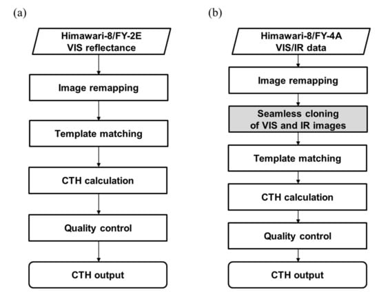
Figure 1.
Flowcharts of (a) the prototype and (b) improved dual-GEO CTH algorithms. The grey rectangle in (b) indicates the additional step with reference to the prototype algorithm.
4. Improved Dual-GEO CTH Algorithm
The improved dual-GEO CTH algorithm adopts a new combination of two GEOs, Himawari-8 and FY-4A. The core of the improved dual-GEO CTH algorithm is similar to that of the prototype algorithm described in Section 3. The main difference is the use of an IR band in addition to the VIS band to more accurately retrieve the heights of the optically thin upper clouds overlying lower clouds. Figure 1b shows the flowchart of the improved dual-GEO CTH algorithm. The grey square in Figure 1 indicates the additional step with reference to the prototype algorithm. In this section, we first describe the two approaches (i.e., VIS-band-based and IR-band-based approaches) to retrieve stereoscopic CTHs by considering a sample case and then discuss the use of an IR band in addition to the VIS band in the improved algorithm.
4.1. Characteristics of VIS-Band-Based and IR-Band-Based Approaches
As mentioned in Section 3, the prototype dual-GEO CTH algorithm adopts the VIS-band-based approach to retrieve stereoscopic CTHs owing to its high horizontal resolution, which significantly influences the retrieval accuracy of stereoscopic CTHs [10]. However, the reflectance in a VIS image is not always observed from a cloud top. For optically thin upper clouds overlying lower clouds, the reflectance characteristics are similar to those of lower clouds. In this case, the VIS-band-based approach may underestimate the stereoscopic CTHs because the parallax of the lower clouds is encountered in the retrieval of the stereoscopic CTHs [24]. Figure 2 and Figure 3 illustrate this problem. Figure 2 shows the AHI false-color RGB image at 03:00 UTC on 12 January 2020. This false-color RGB image corresponds to a combination of AHI bands 3 (0.64 μm for red), 4 (0.86 μm for green), and 14 (11.2 μm, reversed for blue). Yellow, green, black, and light blue regions represent lower clouds, land, ocean, and upper clouds, respectively. The optically thin upper clouds overlying the lower clouds are aligned in the northeast direction from 19°N. Figure 3a,c show the AHI band 3 (0.64 μm) and 7 (3.9 μm) images at 03:00 UTC on 12 January 2020, respectively. Figure 3b shows the VIS-band-based stereoscopic CTHs for this scene. The VIS-band-based approach partially retrieves the heights of the optically thin upper clouds, and the values pertain mainly to the lower clouds, especially near 19–21°N, 110–112°E and 23–25°N, 118–120°E. This finding indicates that lower clouds under the optically thin upper clouds impact the retrieval of the VIS-band-based stereoscopic CTHs.
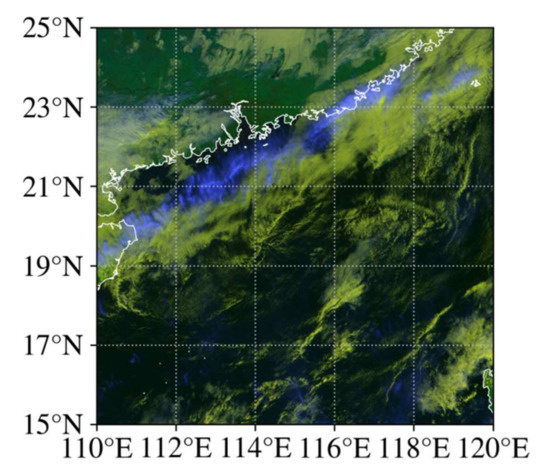
Figure 2.
AHI false-color RGB image at 03:00 UTC on 12 January 2020. This image corresponds to a combination of the AHI bands 3 (red), 4 (green), and 14 (blue, reversed).
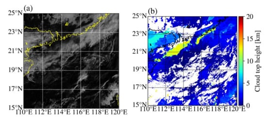
Figure 3.
Satellite images and derived cloud-top heights (CTHs) at 03:00 UTC on 12 January 2020. (a) AHI band 3 (0.64 μm) image. (b) Corresponding VIS-band-based stereoscopic CTHs. (c) AHI band 7 (3.9 μm) image. (d) Corresponding IR-band-based stereoscopic CTHs. (e) Result of seamless image cloning of (a,c). (f) Stereoscopic CTHs based on the cloned image.
Because optically thin upper clouds can be clearly detected in IR images, the IR-band-based approach may be a promising alternative. However, the IR band of a GEO satellite has a coarse horizontal resolution, resulting in a low retrieval accuracy of the stereoscopic CTHs. Figure 3d shows the IR-band-based stereoscopic CTHs for the same scene as that considered for the VIS-band-based approach. The IR-band-based approach successfully retrieves the heights of the optically thin upper clouds overlying the lower clouds. However, the overall quality of the stereoscopic CTH is low. This finding indicates that the coarser horizontal resolution of the IR band of the GEO satellite reduces the retrieval accuracy of stereoscopic CTHs.
In summary, the two approaches have inherent advantages and disadvantages. The VIS-band-based approach exhibits high retrieval accuracy for the stereoscopic CTHs; however, the obtained CTHs tend to be underestimated when the reflectance is not observed from a cloud top, as in the case of optically thin upper clouds overlying lower clouds. In contrast, although the IR-band-based approach can retrieve the stereoscopic CTHs of optically thin upper clouds overlying lower clouds, the overall retrieval accuracy of the stereoscopic CTH is low.
4.2. Seamless Image Cloning
The proposed strategy exploits the advantages of the two approaches, as mentioned in Section 4.1, by applying an image blending technique to VIS and IR images. The key concept is to simultaneously consider VIS and IR characteristics in one image obtained via image blending and use the blended images to retrieve the stereoscopic CTHs. Notably, when the VIS and IR images are blended, most of the characteristics of the VIS band are preserved in the blended image, and the area that is difficult to represent in the VIS band is replaced by the IR characteristics. In this study, as the image blending technique, seamless image cloning [35] is adopted. Using this approach, a source image can be seamlessly cloned over a target image. In this section, we briefly review the seamless image cloning approach reported in [35]. The seamless image cloning method aims to preserve the gradient of the source image as much as possible in the cloned image while matching the target image at the source boundary. Figure 4 shows the schematic and notations of the seamless image cloning approach. is the closed subset (the inserted image) of the target image with boundary . and are known scalar functions for the target and source image, respectively. is an unknown scalar function over the interior of . Seamless image cloning is performed by solving the minimization problem defined in Equation (1).
where is the gradient operator. The problem is to identify the unknown scalar function over the interior of . The solution of Equation (1) is the unique solution of the following Poisson equation with Dirichlet boundary conditions:
where is the Laplacian operator. Because the image intensities are defined on discrete grids (pixels), Equation (2) can be discretized and solved using various iterative algorithms such as the Gauss-Seidel method.
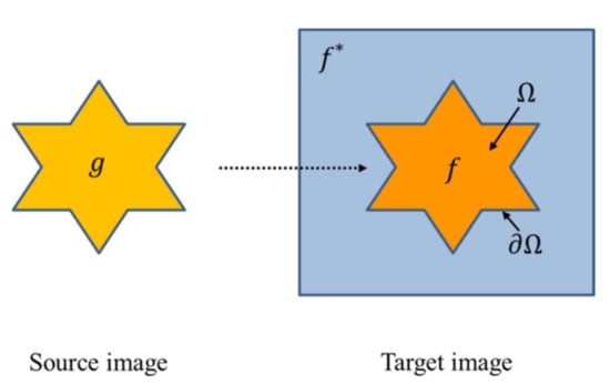
Figure 4.
Schematic and notations of seamless image cloning. The source image is cloned into the enclosed area of the target image with seamless image cloning. In the figure above, the target image is not the cloned image, but the image from which the clone of the source image is performed.
Two spectral bands associated with the VIS and IR bands are required to perform seamless image cloning. These bands must be suitable for presenting cloud structures. Among the bands available from the two satellites, we select the red band (AHI band 3/AGRI band 2) and shortwave IR window band (AHI band 7/AGRI band 7). The red band has the finest horizontal resolution (0.5 km at the SSP) among the available VIS bands and can thus most precisely represent the cloud textures. The shortwave IR window band can represent the cloud-top features based on the differences in thermal radiation. The longwave IR window band (e.g., 11 μm) may also be used for this purpose. However, the horizontal resolution of the AHI longwave IR window band is 2 km, whereas that of the AGRI longwave IR window band is 4 km. In other words, the AGRI has a disadvantage in presenting cloud features compared to the AHI. Therefore, among the available IR window bands, we choose the shortwave IR band with the same horizontal resolution on both instruments.
To perform seamless image cloning, we match the horizontal resolutions of the VIS and IR images. In general, two approaches can be used to match the horizontal resolution. First, a fine-resolution VIS image can be aggregated to a coarser horizontal resolution of an IR image. Second, a coarse-resolution IR image can be resampled to the pixel size of a fine-resolution VIS image. In this study, the latter approach based on the bi-cubic interpolation method is used.
The reflectance range of a VIS image is different from the brightness temperature range of an IR image, and the units of the values are also different. Therefore, we normalize the VIS reflectance and IR brightness temperature after matching the horizontal resolutions of the VIS and IR images. Specifically, the VIS reflectance defined at every pixel is normalized to the 8-bit range (0–255) using Equation (3):
where and are the minimum and maximum VIS reflectance values in the target area, respectively. is the normalized VIS reflectance. The IR brightness temperature is normalized similar to the VIS reflectance but reversed to present the cold feature bright. Equation (4) presents the formula to normalize the IR brightness temperature.
where and are the minimum and maximum IR brightness temperatures in the target area, respectively. is the normalized IR brightness temperature.
Finally, the normalized IR image is blended with the normalized VIS image via seamless image cloning. Figure 3e shows the resulting blended image of the VIS (Figure 3a) and IR images (Figure 3c). The intensities of the blended image are similar to those of the VIS image. However, in the region of the optically thin upper clouds overlying the lower clouds, the intensities of the IR image are shown. Note that the intensities of the optically thin upper clouds overlying the lower clouds in the resulting blended image are not the same as those in the IR image. As mentioned previously, seamless image cloning does not preserve the intensities of a source image in a target image. Instead, the gradients of the resulting image are similar to those of the source image. Figure 3f shows the resulting stereoscopic CTHs from the improved dual-GEO CTH algorithm. The properties of the retrieved stereoscopic CTHs are similar to those corresponding to the VIS-band-based approach (Figure 3b), and the heights of the optically thin upper clouds overlying lower clouds can be retrieved.
5. Inter-Comparison between Operational CTH Products
Section 4 discusses the potential for retrieving the heights of optically thin upper clouds overlying lower clouds based on the seamless image cloning of VIS and IR images. In this section, the improved dual-GEO CTH algorithm was applied to three scenarios involving upper clouds overlying lower clouds. The retrieved stereoscopic CTHs were compared to the CALIOP and CPR CTHs based on different measurement techniques. Moreover, the results for the AHI CTHs were considered to facilitate an indirect comparison, although the detailed analysis for the AHI CTHs is beyond the scope of this research.
5.1. Case 1: 27 February 2019
Figure 5 shows the retrieval results for the first case corresponding to 05:00 UTC on 27 February 2019. The prototype VIS-band-based stereoscopic CTHs and proposed stereoscopic CTHs with the CALIPSO/CloudSat track (red dashed line) are shown in Figure 5a,b, respectively. The retrieval patterns of the two stereoscopic CTHs were similar, albeit with certain differences. The prototype dual-GEO CTH algorithm could not detect several upper clouds (e.g., 33–35°N and 123–124°E, 32–33°N and 127–128°E, 36–37°N and 127–128°E). In contrast, the proposed algorithm successfully detected these clouds. Although the AHI also detected these clouds, the retrieved CTHs were slightly underestimated compared to those obtained using the proposed algorithm (Figure 5c). This is evident in Figure 5d, which shows the differences between the improved dual-GEO CTHs and AHI CTHs. Figure 5e shows the vertical cross-section of the CPR reflectivity and five CTHs from the CALIOP (purple circles), CPR (red diamonds), AHI (black squares), prototype dual-GEO CTH algorithm (green triangles), and improved dual-GEO CTH algorithm (orange inverted triangles). Figure 5f presents the CALIOP cloud boundary information. According to the CPR reflectivity and CALIOP cloud boundary information, upper clouds overlying lower clouds were present from 31°N to 35°N along the CALIPSO/CloudSat track. This region could be divided into 31–33°N and 3–35°N according to the characteristics of the upper clouds. In the region from 31°N to 33°N, the CALIOP backscatter signals were completely attenuated by the optically thick upper clouds (Figure 5f). The five retrieval results for these clouds were similar to one another.
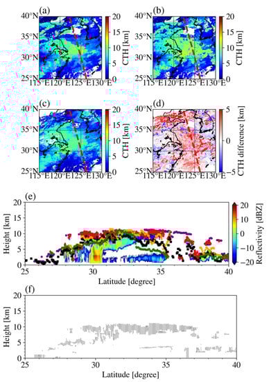
Figure 5.
CTHs obtained using the (a) prototype and (b) improved dual-GEO algorithm at 05:00 UTC on 27 February 2019. The CALIPSO/CloudSat track (red dashed line) is superimposed. (c) AHI CTHs. (d) Differences between the improved dual-GEO CTHs and AHI CTHs. (e) CPR 94 GHz reflectivity, and five CTHs from the CALIOP (purple circles), CPR (red diamonds), AHI (black squares), prototype dual-GEO CTH algorithm (green triangles), and improved dual-GEO CTH algorithm (orange inverted triangles) along the CALIPSO/CloudSat track. (f) CALIOP cloud boundary information.
In the region from 33°N to 35°N, the upper clouds were optically thin, and the prototype dual-GEO CTH algorithm retrieved the heights of lower clouds instead of those of the upper clouds. As mentioned previously, this phenomenon occurred because the parallax of lower clouds affected the retrieval of the stereoscopic CTHs by the prototype dual-GEO CTH algorithm. In contrast, the improved dual-GEO CTH algorithm could retrieve the heights of the upper clouds. The CALIOP and CPR successfully retrieved the heights of the upper clouds, and the retrieved heights were similar to one another. The AHI tended to retrieve the mid-heights between the two cloud layers. In general, in the case of two-layered clouds, the retrieved CTHs from a passive instrument were representative of the radiative mean between the two cloud layers [36,37]. This result is consistent with that reported by Huang et al. [38], which evaluated the AHI CTHs using shipborne radar-lidar merged products and the CALIOP CTHs. It is noted that for the regions from 35°N to 40°N, the proposed algorithm generally retrieved the heights of lower clouds rather than those of the upper clouds, which were optically extremely thin or extremely small. This result could be attributed to the low sensitivity of the passive IR instrument to these clouds. This finding indicates that the performance of the proposed algorithm may not be satisfactory when the upper clouds are optically extremely thin or have an extremely small size. For the optically thick clouds from 28°N to 31°N, the retrieved CTHs were in agreement. Several studies have shown that the retrieval performances associated with the CALIOP, CPR, and passive instruments, such as the AHI and AGRI, are similar in the case of optically thick clouds [4,38,39]. The two stereoscopic CTHs were similar to each other.
Figure 6a,b respectively present the probability densities of the CTH differences pertaining to the three CTHs from the AHI (black), prototype dual-GEO CTH algorithm (green), and improved dual-GEO CTH algorithm (orange), and the CALIOP/CPR CTHs for this case. Retrievals were considered when the AHI, prototype dual-GEO CTH algorithm, and improved dual-GEO CTH algorithm, as well as the CALIOP/CPR, provided CTHs. The numbers of comparison datasets for the CALIOP and CPR CTHs were 489 and 413, respectively. The improved dual-GEO CTHs were more similar to the CALIOP/CPR CTHs compared to the previous dual-GEO CTHs. To further investigate the CTH behaviors for different numbers of cloud layers, the cloud cases were separated into cases with single-layer and multi-layer clouds considering the number of layers in the CALIOP level 2 data. Figure 6c,d shows the results of the single-layer clouds for the CALIOP (249 comparison pairs) and CPR (249 comparison pairs), respectively. Figure 6d,e shows the results of the multi-layer clouds for the CALIOP (240 comparison pairs) and CPR (164 comparison pairs), respectively. As expected, the proposed algorithm achieved superior results for the multi-layer clouds compared to those obtained using the prototype algorithm. Moreover, the improved dual-GEO CTHs were more similar to the CPR CTHs than the CALIOP CTHs.
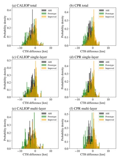
Figure 6.
Probability densities of the CTH difference for three CTHs (AHI, prototype dual-GEO CTH algorithm, and improved dual-GEO CTH algorithm) and CALIOP/CPR CTHs at 05:00 UTC on 27 February 2019. Panels (a,b) show the probability densities of CTH differences for the total clouds, compared to the CALIOP, and CPR CTHs, respectively. Panels (c,d) show the results for single-layer clouds, and panels (e,f) show the results for multi-layer clouds.
Table 2 summarizes the inter-comparison statistics for the three CTHs derived from the AHI, prototype dual-GEO CTH algorithm, and improved dual-GEO CTH algorithm with the CALIOP/CPR CTHs for this case. The considered statistics are the mean absolute error (MAE), mean bias error (MBE), and root mean square error (RMSE). All three statistics indicated that the improved dual-GEO CTHs were more similar to the CALIOP or CPR CTHs, compared with the prototype dual-GEO CTHs. This trend was more evident in the case of multi-layered clouds, as confirmed in Figure 6.
Table 2.
Statistics for three CTHs derived from the AHI, prototype dual-GEO CTH algorithm, and improved dual-GEO CTH algorithm with the CALIOP and CPR CTHs at 05:00 UTC on 27 February 2019. Statistics are shown for the cloud regimes: total, single-layer, and multi-layer clouds. MAE, MBE, and RMSE represent the mean absolute error, mean bias error, and root mean square error, respectively, presented in units of km.
5.2. Case 2: 3 December 2018
Figure 7 presents the retrieval results for the second case pertaining to 05:00 UTC on 3 December 2018. The prototype dual-GEO CTH algorithm did not detect upper clouds over the Korean peninsula (Figure 7a). In contrast, the proposed algorithm detected these upper clouds (Figure 7b). The AHI also detected these upper clouds, although the retrieved CTHs were smaller than those obtained using the improved dual-GEO CTH algorithm (Figure 7c,d). According to the CPR reflectivity and CALIOP cloud boundary information (Figure 7e,f), upper clouds overlying lower clouds were present from 36.5°N to 40°N along the CALIPSO/CloudSat track. In the areas north of 38°N, the proposed algorithm more accurately retrieved the heights of the upper clouds compared to those obtained using the prototype dual-GEO CTH algorithm and AHI. However, for the regions from 36.5°N to 38°N, the proposed algorithm retrieved the heights of lower clouds rather than those of the upper clouds, which were optically extremely thin or extremely small. This result was consistent with that of case study 1 (Section 5.1). For optically thick clouds (31°N to 35.5°N) and low clouds (35.5°N to 36°N), the retrieved CTHs were generally similar to one another.
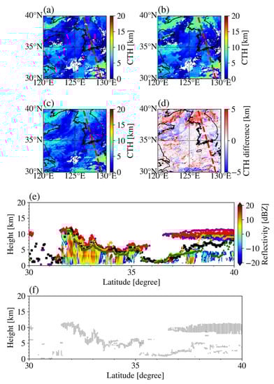
Figure 7.
CTHs obtained using the (a) prototype and (b) improved dual-GEO algorithm at 05:00 UTC on 3 December 2018. The CALIPSO/CloudSat track (red dashed line) is superimposed. (c) AHI CTHs. (d) Differences between the improved dual-GEO CTHs and AHI CTHs. (e) CPR 94 GHz reflectivity, and five CTHs from the CALIOP (purple circles), CPR (red diamonds), AHI (black squares), prototype dual-GEO CTH algorithm (green triangles), and improved dual-GEO CTH algorithm (orange inverted triangles) along the CALIPSO/CloudSat track. (f) CALIOP cloud boundary information.
Figure 8 shows the same probability densities of the CTH differences as those shown in Figure 6, but for the second case. The total numbers of comparison datasets for the CALIOP and CPR CTHs were 365 and 331, respectively. For single-layer (multi-layer) clouds, the numbers of comparison datasets for the CALIOP and CPR CTHs were 202 (163) and 243 (88), respectively. The results showed that the proposed algorithm outperformed the prototype algorithm (Figure 8a,b), and this trend was especially evident in the case involving multi-layer clouds (Figure 8e,f). It is also noted that the probability densities of CTH differences were bimodal. The secondary peaks of the probability densities for dual-GEO CTHs were evident in the multi-layer clouds. This is likely because the CALIOP and CPR retrieved the heights of the upper cloud of multi-layer clouds, while the dual-GEO CTH algorithms tend to retrieve heights of the lower cloud (e.g., clouds between 36.5°N and 38°N), as mentioned above. The secondary peaks of the probability densities for the AHI CTHs were also evident in the multi-layer clouds. This is because the AHI tends to retrieve the mid-heights between two cloud layers. This result is consistent with that reported by previous studies [38,40].
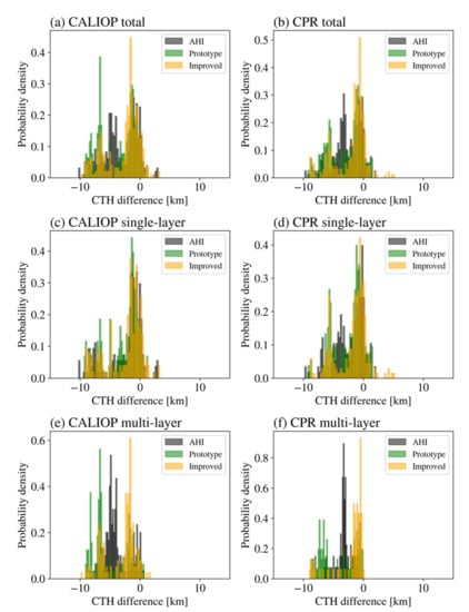
Figure 8.
Probability densities of the CTH difference for three CTHs (AHI, prototype dual-GEO CTH algorithm, and improved dual-GEO CTH algorithm) and CALIOP/CPR CTHs at 05:00 UTC on 3 December 2018. Panels (a,b) show the probability densities of CTH differences for the total clouds, compared to the CALIOP, and CPR CTHs, respectively. Panels (c,d) show the results for single-layer clouds, and panels (e,f) show the results for multi-layer clouds.
Table 3 summarizes the same statistics as those presented in Table 2, but for the second case. All three statistics showed that the proposed algorithm outperformed the prototype algorithm, and this aspect was more evident in the case with multi-layer clouds. However, the statistics were inferior to those in the first case. This phenomenon could likely be attributed to the influence of the clouds present from 36.5°N to 38°N, as mentioned previously.
Table 3.
Statistics for three CTHs derived from the AHI, prototype dual-GEO CTH algorithm, and improved dual-GEO CTH algorithm with the CALIOP and CPR CTHs at 05:00 UTC on 3 December 2018. Statistics are shown for the cloud regimes: total, single-layer, and multi-layer clouds. MAE, MBE, and RMSE represent the mean absolute error, mean bias error, and root mean square error, respectively, presented in units of km.
5.3. Case 3: 10 January 2019
Figure 9 presents the final retrieval results at 06:00 UTC on 10 January 2019. In this case, the retrieval patterns of the two stereoscopic CTHs were similar to each other. However, the heights of the upper clouds near 22°N were retrieved only by the proposed algorithm (Figure 9b) and not by the prototype algorithm (Figure 9a). The retrieval patterns associated with the proposed dual-GEO CTHs were similar to the AHI CTHs (Figure 9c), and the heights of the upper clouds were slightly smaller than those obtained using the proposed algorithm (Figure 9d). According to the CPR reflectivity and CALIOP cloud boundary information (Figure 9e,f), optically thin upper clouds (~10 km) overlying lower clouds were present near the surface near 22°N. The CALIOP and CPR detected these upper clouds, and the retrieved CTHs were similar to each other. However, the prototype dual-GEO CTH algorithm retrieved the heights of the lower clouds rather than those of the upper clouds. As mentioned previously, this phenomenon likely occurred because the parallax of the lower clouds affected the retrieval of the stereoscopic CTHs. In contrast, the proposed algorithm detected the upper clouds, and the retrieved heights were comparable to those of the CALIOP and CPR CTHs. The AHI CTHs for these clouds were mid-heights of the two cloud layers, as mentioned in Section 5.1. For the clouds from 20°N to 21°N, the proposed algorithm retrieved the heights of the lower clouds near the surface rather than those of the upper clouds. This result was similar to that in the cases described in Section 5.1 and Section 5.2. In particular, in the presence of optically extremely thin or extremely small upper clouds, the performance of the proposed algorithm was not entirely adequate. For the optically thick clouds from 26°N to 30°N, the five CTHs were in agreement. For the optically thin low clouds near the surface from 22°N to 25°N, the CALIOP and CPR CTHs were similar to each other, but the CPR did not detect certain clouds due to the ground clutter near the surface. Moreover, the AHI CTHs were similar to the CALIOP and CPR CTHs, and the two stereoscopic CTHs were slightly smaller than the CALIOP and CPR CTHs.
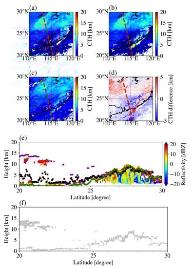
Figure 9.
CTHs obtained using the (a) prototype and (b) improved dual-GEO algorithm at 06:00 UTC on 10 January 2019. The CALIPSO/CloudSat track (red dashed line) is superimposed. (c) AHI CTHs. (d) Differences between the improved dual-GEO CTHs and AHI CTHs. (e) CPR 94 GHz reflectivity, and five CTHs from the CALIOP (purple circles), CPR (red diamonds), AHI (black squares), prototype dual-GEO CTH algorithm (green triangles), and improved dual-GEO CTH algorithm (orange inverted triangles) along the CALIPSO/CloudSat track. (f) CALIOP cloud boundary information.
Figure 10 shows the same probability densities of the CTH differences as those shown in Figure 6, but for the final case. The total numbers of comparison datasets for the CALIOP and CPR CTHs were 380 and 220, respectively. For single-layer (multi-layer) clouds, the numbers of comparison datasets for the CALIOP and CPR CTHs were 204 (120) and 176 (100), respectively. The differences between the prototype dual-GEO CTHs and CALIOP CTHs (Figure 10a) pertained to a peak slightly less than zero. The secondary peaks were also found around −15 km. These secondary peaks could be attributed to the presence of the optically extremely thin clouds from 20°N to 22°N (Figure 9e). The CALIOP retrieved the heights of these upper clouds, but the prototype dual-GEO CTH algorithm retrieved the heights of lower clouds. This result, once again, is consistent with that of case study 2 (Section 5.2). The behaviors associated with the improved dual-GEO CTHs were similar to those of the prototype dual-GEO CTHs, although the differences with the CALIOP CTHs were reduced. The secondary peaks for the AHI CTHs were also found because the AHI generally retrieved the mid-heights between two layers. The improvements in the algorithm were more notable in comparison with the CPR CTHs (Figure 10b). Moreover, for the different numbers of cloud layers (Figure 10c–f), the proposed algorithm outperformed the prototype algorithm, especially in the case of multi-layer clouds.
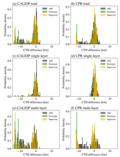
Figure 10.
Probability densities of the CTH difference for three CTHs (AHI, prototype dual-GEO CTH algorithm, and improved dual-GEO CTH algorithm) and CALIOP/CPR CTHs at 06:00 UTC on 10 January 2019. Panels (a,b) show the probability densities of CTH differences for the total clouds, compared to the CALIOP, and CPR CTHs, respectively. Panels (c,d) show the results for single-layer clouds, and panels (e,f) show the results for multi-layer clouds.
Table 4 summarizes the same statistics as those presented in Table 2, but for the final case. In this case, the proposed algorithm outperformed the prototype algorithm, especially in the case involving multi-layer clouds.
Table 4.
Statistics for three CTHs derived from the AHI, prototype dual-GEO CTH algorithm, and improved dual-GEO CTH algorithm with the CALIOP and CPR CTHs at 06:00 UTC on 10 January 2019. Statistics are shown for the cloud regimes: total, single-layer, and multi-layer clouds. MAE, MBE, and RMSE represent the mean absolute error, mean bias error, and root mean square error, respectively, presented in units of km.
6. Discussion and Conclusions
The prototype dual-GEO CTH algorithm [16] adopts the VIS-band-based approach to retrieve stereoscopic CTHs. This algorithm can retrieve reliable stereoscopic CTHs, but tends to underestimate the heights of optically thin upper clouds overlying lower clouds. This is a fundamental weakness of the VIS-band-based approach. Because optically thin upper clouds are transparent, the VIS-band-based approach tends to detect the parallax shift of lower clouds, resulting in underestimation of heights for optically thin upper clouds overlying lower clouds. To address this problem, this paper proposes an improved dual-GEO CTH algorithm for Himawari-8 and FY-4A GEOs.
The basic principle of the proposed algorithm is similar to that of the prototype algorithm: the prototype and improved dual-GEO CTH algorithms determine the parallax shift from two simultaneous images and converts the parallax shift to stereoscopic CTHs. The main difference is that the proposed algorithm, in addition to the VIS band, employs the IR band to more accurately retrieve the stereoscopic heights of optically thin upper clouds overlying lower clouds. Specifically, the proposed algorithm implements seamless image cloning to blend the VIS and IR images. Because the VIS-band-based approach can retrieve reliable stereoscopic CTHs, most characteristics of the VIS band are preserved in the blended image. Instead, the area that is difficult to represent in the VIS band (i.e., optically thin upper clouds overlying lower clouds) is replaced by IR characteristics. The resulting blended image can better represent the optically thin upper clouds overlying lower clouds than the VIS image while retaining the characteristics of the VIS band. This indicates that a more reliable parallax shift can be detected in the blended image, which enables more accurate stereoscopic CTH retrieval compared to the VIS-band-based approach.
The improved dual-GEO CTH algorithm is evaluated by comparing the CALIOP and CPR CTHs for three cases involving upper clouds overlying lower clouds. The proposed algorithm outperforms the prototype algorithm, and the improvement is especially evident in cases involving upper clouds overlying lower clouds, as expected. To obtain more reliable results, more detailed inter-comparisons are required. This will be included in future work.
The proposed algorithm involves certain limitations. First, the improved dual-GEO CTH algorithm is a daytime algorithm. Specifically, the algorithm uses a VIS band, which limits its use at night. Second, the performance of the proposed algorithm may not be adequate when the upper clouds are optically extremely thin or extremely small (Section 5). This phenomenon can be attributed to the low sensitivity of the passive IR instruments adopted by the proposed algorithm for these clouds. The application of a detailed multi-layer cloud detection, such as in Wang et al. [41] and Teng et al. [42], would be helpful for further improvements of our algorithm. This will be considered in future work.
Although the proposed algorithm has been designed for Himawari-8 and FY-4A GEOs, it can be used for any combination of two GEOs. As mentioned in Section 4, the proposed algorithm uses a shortwave IR window band as an additional IR band because the horizontal resolutions of the AGRI IR bands are relatively lower than those of the AHI IR bands. If the horizontal resolutions of the IR bands are higher, other IR window bands, such as a longwave IR window band, may be used.
Author Contributions
J.-h.L. developed the algorithm and wrote the original manuscript. D.-B.S. designed the experiments and reviewed and edited the manuscript. All authors have read and agreed to the published version of the manuscript.
Funding
This work was supported by the National Research Foundation of Korea (NRF) through a grant funded by the Korean government (MSIT) (no. 2020R1A4A1016537).
Institutional Review Board Statement
Not applicable.
Informed Consent Statement
Not applicable.
Data Availability Statement
Publicly available datasets were used in this study. The Himawari-8 full disk data are available from ftp://hmwr829gr.cr.chiba-u.ac.jp. The FY-4A full disk data are available from https://satellite.nsmc.org.cn. The CALIOP level 2 5-km cloud layer data are available from http://search.earthdata.nasa.gov. The CPR level 2 geometric profile data are available from http://www.cloudsat.cira.colostate.edu. The AHI operational cloud property products are available from https://www.eorc.jaxa.jp/ptree. All data were accessed finally on 24 October 2021.
Acknowledgments
The authors would like to thank the editor and anonymous reviewers for their helpful comments and suggestions that have helped enhance the quality of the manuscript. FY-4A and Himawari-8 full-disk data were obtained from the FENGYUN Satellite Data Center of the National Satellite Meteorological Center and Center for Environmental Remote Sensing at Chiba University, respectively. The CALIOP level 2 5-km cloud layer data product, CPR level 2 geometric profile data product, and AHI official cloud property product were obtained from the National Aeronautics and Space Administration Earthdata, CloudSat Data Processing Center, and Japan Aerospace Exploration Agency P-Tree system, respectively.
Conflicts of Interest
The authors declare no conflict of interest.
References
- Cheng, X.; Yi, L.; Bendix, J. Cloud top height retrieval over the Arctic Ocean using a cloud-shadow method based on MODIS. Atmos. Res. 2021, 253, 105468. [Google Scholar] [CrossRef]
- Wielicki, B.A.; Coakley, J.A. Cloud retrieval using infrared sounder data: Error analysis. J. Appl. Meteorol. Climatol. 1981, 20, 157–169. [Google Scholar] [CrossRef] [Green Version]
- Menzel, W.P.; Smith, W.L.; Stewart, T.R. Improved cloud motion wind vector and altitude assignment using VAS. J. Appl. Meteorol. Climatol. 1983, 22, 377–384. [Google Scholar] [CrossRef]
- Hamann, U.; Walther, A.; Baum, B.; Bennartz, R.; Bugliaro, L.; Derrien, M.; Francis, P.N.; Heidinger, A.; Joro, S.; Kniffka, A.; et al. Remote sensing of cloud top pressure/height from SEVIRI: Analysis of ten current retrieval algorithms. Atmos. Meas. Tech. 2014, 7, 2839–2867. [Google Scholar] [CrossRef] [Green Version]
- Winker, D.M.; Vaughan, M.A.; Omar, A.; Hu, Y.; Powell, K.A.; Liu, Z.; Hunt, W.H.; Young, S.A. Overview of the CALIPSO mission and CALIOP data processing algorithms. J. Atmos. Ocean. Technol. 2009, 26, 2310–2323. [Google Scholar] [CrossRef]
- Stephens, G.L.; Vane, D.G.; Boain, R.J.; Mace, G.G.; Sassen, K.; Wang, Z.; Illingworth, A.J.; O’Connor, E.J.; Rossow, W.B.; Durden, S.L.; et al. The CLOUDSAT Mission and the A-Train: A new dimension of space-based observations of clouds and precipitation. Bull. Am. Meteorol. Soc. 2002, 83, 1771–1790. [Google Scholar] [CrossRef] [Green Version]
- Im, E.; Wu, C.; Durden, S.L. Cloud profiling radar for the CloudSat mission. IEEE Aerosp. Electron. Syst. Mag. 2005, 20, 15–18. [Google Scholar] [CrossRef]
- Stephens, G.L.; Vane, D.G.; Tanelli, S.; Im, E.; Durden, S.; Rokey, M.; Reinke, D.; Partain, P.; Mace, G.G.; Austin, R.; et al. CloudSat mission: Performance and early science after the first year of operation. J. Geophys. Res. Atmos. 2008, 113, D00A18. [Google Scholar] [CrossRef]
- Muller, J.P.; Denis, M.A.; Dundas, R.D.; Mitchell, K.L.; Naud, C.; Mannstein, H. Stereo cloud-top heights and cloud fraction retrieval from ATSR-2. Int. J. Remote Sens. 2007, 28, 1921–1938. [Google Scholar] [CrossRef] [Green Version]
- Zakšek, K.; Hort, M.; Zaletelj, J.; Langmann, B. Monitoring volcanic ash cloud top height through simultaneous retrieval of optical data from polar orbiting and geostationary satellites. Atmos. Chem. Phys. 2013, 13, 2589–2606. [Google Scholar] [CrossRef] [Green Version]
- Hasler, A.F. Stereographic observations from geosynchronous satellites: An important new tool for the atmospheric sciences. Bull. Am. Meteorol. Soc. 1981, 62, 194–212. [Google Scholar] [CrossRef] [Green Version]
- Hasler, A.F.; Strong, J.; Woodward, R.H.; Pierce, H. Automatic analysis of stereoscopic satellite image pairs for determination of cloud-top height and structure. J. Appl. Meteorol. Climatol. 1991, 30, 257–281. [Google Scholar] [CrossRef] [Green Version]
- Wylie, D.P.; Santek, D.; Starr, D.O.C. Cloud-top heights from GOES-8 and GOES-9 stereoscopic imagery. J. Appl. Meteorol. 1998, 37, 405–413. [Google Scholar] [CrossRef]
- Seiz, G.; Tjemkes, S.; Watts, P. Multiview cloud-top height and wind retrieval with photogrammetric methods: Application to Meteosat-8 HRV observations. J. Appl. Meteorol. Climatol. 2007, 46, 1182–1195. [Google Scholar] [CrossRef] [Green Version]
- Merucci, L.; Zakšek, K.; Carboni, E.; Corradini, S. Stereoscopic estimation of volcanic ash cloud-top height from two geostationary satellites. Remote Sens. 2016, 8, 206. [Google Scholar] [CrossRef] [Green Version]
- Lee, J.; Shin, D.-B.; Chung, C.-Y.; Kim, J. A cloud top-height retrieval algorithm using simultaneous observations from the Himawari-8 and FY-2E satellites. Remote Sens. 2020, 12, 1953. [Google Scholar] [CrossRef]
- Carr, J.L.; Wu, D.L.; Daniels, J.; Friberg, M.D.; Bresky, W.; Madani, H. GEO–GEO stereo-tracking of atmospheric motion vectors (AMVs) from the geostationary ring. Remote Sens. 2020, 12, 3779. [Google Scholar] [CrossRef]
- Corradini, S.; Montopoli, M.; Guerrieri, L.; Ricci, M.; Scollo, S.; Merucci, L.; Marzano, F.S.; Pugnaghi, S.; Prestifilippo, M.; Ventress, L.J.; et al. A multi-sensor approach for volcanic ash cloud retrieval and eruption characterization: The 23 november 2013 Etna lava fountain. Remote Sens. 2016, 8, 58. [Google Scholar] [CrossRef] [Green Version]
- Carr, J.L.; Wu, D.L.; Wolfe, R.E.; Madani, H.; Lin, G.; Tan, B. Joint 3D-wind retrievals with stereoscopic views from MODIS and GOES. Remote Sens. 2019, 11, 2100. [Google Scholar] [CrossRef] [Green Version]
- Prata, A.J.; Turner, P.J. Cloud-top height determination using ATSR data. Remote Sens. Environ. 1997, 59, 1–13. [Google Scholar] [CrossRef]
- Moroney, C.; Davies, R.; Muller, J. Operational retrieval of cloud-top heights using MISR data. IEEE Trans. Geosci. Remote Sens. 2002, 40, 1532–1540. [Google Scholar] [CrossRef]
- Nelson, D.L.; Garay, M.J.; Kahn, R.A.; Dunst, B.A. Stereoscopic height and wind retrievals for aerosol plumes with the MISR INteractive eXplorer (MINX). Remote Sens. 2013, 5, 4593–4628. [Google Scholar] [CrossRef] [Green Version]
- Virtanen, T.H.; Kolmonen, P.; Rodríguez, E.; Sogacheva, L.; Sundström, A.M.; de Leeuw, G. Ash plume top height estimation using AATSR. Atmos. Meas. Tech. 2014, 7, 2437–2456. [Google Scholar] [CrossRef] [Green Version]
- Fisher, D.; Poulsen, C.A.; Thomas, G.E.; Muller, J.P. Synergy of stereo cloud top height and ORAC optimal estimation cloud retrieval: Evaluation and application to AATSR. Atmos. Meas. Tech. 2016, 9, 909–928. [Google Scholar] [CrossRef] [Green Version]
- Castro, E.; Ishida, T.; Takahashi, Y.; Kubota, H.; Perez, G.J.; Marciano, J.S. Determination of cloud-top height through three-dimensional cloud reconstruction using DIWATA-1 Data. Sci. Rep. 2020, 10, 7570. [Google Scholar] [CrossRef] [PubMed]
- Bessho, K.; Date, K.; Hayashi, M.; Ikeda, A.; Imai, T.; Inoue, H.; Kumagai, Y.; Miyakawa, T.; Murata, H.; Ohno, T.; et al. An introduction to Himawari-8/9—Japan’s new-generation geostationary meteorological satellites. J. Meteorol. Soc. Jpn. Ser. II 2016, 94, 151–183. [Google Scholar] [CrossRef] [Green Version]
- Yamamoto, Y.; Ichii, K.; Higuchi, A.; Takenaka, H. Geolocation accuracy assessment of Himawari-8/AHI imagery for application to terrestrial monitoring. Remote Sens. 2020, 12, 1372. [Google Scholar] [CrossRef]
- Takenaka, H.; Sakashita, T.; Higuchi, A.; Nakajima, T. Geolocation correction for geostationary satellite observations by a phase-only correlation method using a visible channel. Remote Sens. 2020, 12, 2472. [Google Scholar] [CrossRef]
- Yang, J.; Zhang, Z.; Wei, C.; Lu, F.; Guo, Q. Introducing the new generation of Chinese geostationary weather satellites, Fengyun-4. Bull. Am. Meteorol. Soc. 2017, 98, 1637–1658. [Google Scholar] [CrossRef]
- Mace, G. Level 2 GEOPROF Product Process Description and Interface Control Document Algorithm Version 5.3; NASA Jet Propulsion Laboratory: Pasadena, CA, USA, 2007; p. 44. [Google Scholar]
- Nakajima, T.Y.; Nakajma, T. Wide-area determination of cloud microphysical properties from NOAA AVHRR measurements for FIRE and ASTEX regions. J. Atmos. Sci. 1995, 52, 4043–4059. [Google Scholar] [CrossRef] [Green Version]
- Letu, H.; Nagao, T.M.; Nakajima, T.Y.; Riedi, J.; Ishimoto, H.; Baran, A.J.; Shang, H.; Sekiguchi, M.; Kikuchi, M. Ice cloud properties from Himawari-8/AHI next-generation geostationary satellite: Capability of the AHI to monitor the DC cloud generation process. IEEE Trans. Geosci. Remote Sens. 2018, 57, 3229–3239. [Google Scholar] [CrossRef]
- Letu, H.; Yang, K.; Nakajima, T.Y.; Ishimoto, H.; Nagao, T.M.; Riedi, J.; Baran, A.J.; Ma, R.; Wang, T.; Shang, H. High-resolution retrieval of cloud microphysical properties and surface solar radiation using Himawari-8/AHI next-generation geostationary satellite. Remote Sens. Environ. 2020, 239, 111583. [Google Scholar] [CrossRef]
- Zhuge, X.Y.; Zou, X.L.; Wang, Y. A fast cloud detection algorithm applicable to monitoring and nowcasting of daytime cloud systems. IEEE Trans. Geosci. Remote Sens. 2017, 55, 6111–6119. [Google Scholar] [CrossRef]
- Perez, P.; Gangnet, M.; Blake, A. Poisson image editing. ACM Trans. Graph. 2003, 22, 313–318. [Google Scholar] [CrossRef]
- Weisz, E.; Li, J.; Menzel, W.P.; Heidinger, A.K.; Kahn, B.H.; Liu, C.Y. Comparison of AIRS, MODIS, CloudSat and CALIPSO cloud top height retrievals. Geophys. Res. Lett. 2007, 34, L17811. [Google Scholar] [CrossRef]
- Menzel, W.P.; Frey, R.A.; Zhang, H.; Wylie, D.P.; Moeller, C.C.; Holz, R.E.; Maddux, B.; Baum, B.A.; Strabala, K.I.; Gumley, L.E. MODIS global cloud-top pressure and amount estimation: Algorithm description and results. J. Appl. Meteorol. Climatol. 2008, 47, 1175–1198. [Google Scholar] [CrossRef] [Green Version]
- Huang, Y.; Siems, S.; Manton, M.; Protat, A.; Majewski, L.; Nguyen, H. Evaluating Himawari-8 cloud products using shipborne and CALIPSO observations: Cloud-top height and cloud-top temperature. J. Atmos. Ocean. Technol. 2019, 36, 2327–2347. [Google Scholar] [CrossRef] [Green Version]
- Liu, B.; Huo, J.; Lyu, D.R.; Wang, X. Assessment of FY-4A and Himawari-8 cloud top height retrieval through comparison with ground-based millimeter radar at sites in Tibet and Beijing. Adv. Atmos. Sci. 2021, 38, 1334–1350. [Google Scholar] [CrossRef]
- Li, Q.; Sun, X.; Wang, X. Reliability evaluation of the joint observation of cloud top height by FY-4A and Himawari-8. Remote Sens. 2021, 13, 3851. [Google Scholar] [CrossRef]
- Wang, J.J.; Liu, C.; Yao, B.; Min, M.; Letu, H.S.; Yin, Y.; Yung, Y.L. A multilayer cloud detection algorithm for the Suomi-NPP Visible Infrared Imager Radiometer Suite (VIIRS). Remote Sens. Environ. 2019, 227, 1–11. [Google Scholar] [CrossRef]
- Teng, S.W.; Liu, C.; Zhang, Z.B.; Wang, Y.; Sohn, B.J.; Yung, Y.L. Retrieval of ice-over-water cloud microphysical and optical properties using passive radiometers. Geophys. Res. Lett. 2020, 47, e2020GL088941. [Google Scholar] [CrossRef]
Publisher’s Note: MDPI stays neutral with regard to jurisdictional claims in published maps and institutional affiliations. |
© 2021 by the authors. Licensee MDPI, Basel, Switzerland. This article is an open access article distributed under the terms and conditions of the Creative Commons Attribution (CC BY) license (https://creativecommons.org/licenses/by/4.0/).