Explainable Boosting Machines for Slope Failure Spatial Predictive Modeling

Abstract

Machine learning (ML) methods, such as artificial neural networks (ANN), k-nearest neighbors (kNN), random forests (RF), support vector machines (SVM), and boosted decision trees (DTs), may offer stronger predictive performance than more traditional, parametric methods, such as linear regression, multiple linear regression, and logistic regression (LR), for specific mapping and modeling tasks. However, this increased performance is often accompanied by increased model complexity and decreased interpretability, resulting in critiques of their “black box” nature, which highlights the need for algorithms that can offer both strong predictive performance and interpretability. This is especially true when the global model and predictions for specific data points need to be explainable in order for the model to be of use. Explainable boosting machines (EBM), an augmentation and refinement of generalize additive models (GAMs), has been proposed as an empirical modeling method that offers both interpretable results and strong predictive performance. The trained model can be graphically summarized as a set of functions relating each predictor variable to the dependent variable along with heat maps representing interactions between selected pairs of predictor variables. In this study, we assess EBMs for predicting the likelihood or probability of slope failure occurrence based on digital terrain characteristics in four separate Major Land Resource Areas (MLRAs) in the state of West Virginia, USA and compare the results to those obtained with LR, kNN, RF, and SVM. EBM provided predictive accuracies comparable to RF and SVM and better than LR and kNN. The generated functions and visualizations for each predictor variable and included interactions between pairs of predictor variables, estimation of variable importance based on average mean absolute scores, and provided scores for each predictor variable for new predictions add interpretability, but additional work is needed to quantify how these outputs may be impacted by variable correlation, inclusion of interaction terms, and large feature spaces. Further exploration of EBM is merited for geohazard mapping and modeling in particular and spatial predictive mapping and modeling in general, especially when the value or use of the resulting predictions would be greatly enhanced by improved interpretability globally and availability of prediction explanations at each cell or aggregating unit within the mapped or modeled extent.

1. Introduction

For empirical modeling tasks, in which predictor variables and example data are used to build models and make predictions of class membership, class probabilities, or continuous measures, machine learning (ML) algorithms and methods (e.g., k-nearest neighbor (kNN), artificial neural networks (ANN), support vector machines (SVM), random forests (RF), and boosted decision trees (DTs)) may provide improved model performance in comparison to traditional, parametric methods, such as linear regression, multiple linear regression, logistic regression (LR), and Gaussian maximum likelihood [1,2,3]. This is generally attributed to the ability of ML algorithms to characterize patterns in noisy, large, and/or complex datasets and feature spaces without having to make distribution assumptions that are often violated [2]. Unfortunately, this increased predictive power is generally accompanied by increased model complexity and reduced interpretability, leading practitioners and researchers to critique the “black box” nature of these methods and call for the use of more interpretable or “glass box” models. This is especially true when there is an interest in or need to explain what factors contribute most to the prediction and how the response variable is impacted by specific predictor variables. It is also of value for assessing how specific cases, such as each raster cell or aggregating unit across the mapped or modeled landscape, was predicted and what conditions or site characteristics resulted in the prediction [4,5].

In response to these concerns, recent advancements have yielded new methods or adaptions of existing methods that offer more transparent and interpretable results and predictive performance that may be comparable to those obtainable with black box ML methods, such as SVM, RF, and boosted DTs. In this study, we explore the use of explainable boosting machine (EBM) [6,7] for predicting the probability of slope failure (i.e., landslide) occurrence based on topographic predictor variables calculated from a light detection and ranging (LiDAR)-derived digital terrain model (DTM). We compare predictive performance of EBM to LR and common black box machine learning methods (kNN, RF, and SVM), assess how the algorithm responds when the number of training samples is reduced, compare how models trained in one MLRA generalize to the other study areas, and explore the outputs of the model associated with global interpretability (e.g., generated functions for each predictor variable, heat maps associated with included interactions between pairs of predictor variables, and variable importance estimates based on mean absolute score) and local interpretability (e.g., scores for each predictor variable contributing to the final prediction of a new sample or location). In this study, we define slope failures as the movement of a mass of rock, earth, or debris down a slope.

This study is part of a larger project that explores the use of empirical spatial predictive modeling methods and LiDAR-derived terrain variables for creating spatial probabilistic predictive models of slope failure occurrence. In the first component of the study, Maxwell et al. [8], we used the RF algorithm and explored the importance of predictor variables, the value of including additional, non-terrain variables, and the impact of reducing the number of predictor variables and training samples. In the second study in the series, Maxwell et al. [9], we explored how well RF models developed using training samples from different physiographies generalized to other landscapes. This study expands upon our prior studies in the series by evaluating the use of the EBM algorithm as a potentially more interpretable method for obtaining accurate slope failure occurrence predictions over large spatial extents.

2. Background

2.1. Explainable Machine Learning

EBM builds upon or augments generalized additive models (GAMs) (Equation (1)).

ŷ = β₀ + f₁(x₁) + f₂(x₂) + f₃(x₃) + ……. + f_i(x_i)

(1)

In contrast to linear and multiple linear regression, GAMs do not assume a linear relationship between predictor variables and the response variable. Instead, relationships are modeled using smoothing, spline, or other methods. A response variable is predicted by learning an intercept (β₀) along with functions that describe the relationship between the response and each predictor variable. Essentially, the coefficients (β_i) in a multiple linear regression model are replaced with learned functions (f_i) that are not confined to a linear relationship. The model is additive because separate functions are learned for each predictor variable independently, which allows for an examination of the effect of each predictor variable separately [2]. In order to apply GAMs to binary classification problems, as is the case in this study, class logits are predicted as opposed to a continuous variable (Equation (2)). In this equation, p represents the probability of the sample belonging to the positive class, which is assigned a value of 1 while the negative class is assigned a value of 0 [2,10].

$$\log \left(\frac{p\left(x\right)}{1-p\left(x\right)}\right)={\mathsf{\beta }}_0+f_1\left(x_1\right)+f_2\left(x_2\right)+f_3\left(x_3\right)+\dots \dots .+f_{\mathrm{i}}\left(x_{\mathrm{i}}\right)$$

(2)

Although GAM equations are more interpretable than models generated using black box ML methods, which cannot be presented as a single equation and set of functions that describe the estimated relationship between the dependent variable and values of each predictor variable, they are often less accurate [7]. EBM expands upon GAMs to maintain interpretability but improve predictive performance. EBM is a fast implementation of the generalized additive models plus interactions (GA²M) method [6,7,11]. Using GA²M, the function associated with each predictor variable is approximated using many shallow decision trees created with gradient boosting to iteratively improve model performance. More specifically, shallow decision tree generation, learning, and gradient updates are performed using a single predictor variable at a time in a round-robin fashion with a low learning rate [6,7]. Currently, the InterpretML implementation of EBM, which was used in this study, implements log loss for classification and mean square error loss (MSE) for regression as measures of error or loss [6]. Due to the low learning rate, only small updates to the model are made with the addition of each tree. This requires the model to be built by iterating through the training data over thousands of boosting iterations in which each tree only use one predictor variable. The algorithm developers argue that the low learning rate reduces the influence of the order in which features are used while iteratively cycling through the predictor variables using a round-robin method minimizes the impact of co-linearity to maintain interpretability [6,7,11]. To take into account interactions between predictor variables, two-dimensional functions (f_ij(x_i, x_j)) can be learned to relate the response variable to pairs of predictor variables. The subset of available interactions included are selected using the FAST method proposed by Lou et al. [7] that ranks all pairs of predictor variables. Adding interaction terms requires that the additive nature of GAMs be relaxed [2], and interpreting the influence of a single predictor variable will require investigating the associated one-dimensional function and any two-dimensional interaction functions that include the variable of interest [6,7].

Once an ensemble of decision trees is trained using gradient boosting, all trees produced for a single predictor variable are used to predict the training samples and build the function associated with each feature. Once the trees are used to build the function for each predictor variable, they are no longer needed, simplifying inference to new data. Thus, the function associated with each predictor variable or interaction is derived from the large set of shallow trees as opposed to using a spline method, as is common for traditional GAMs. For binary classification and associated class probabilities, the final prediction is derived by adding all scores (i.e., the effect of each included factor on the predicted logits for the positive class) estimated using each predictor variable and included interactions with the use of a link function to adapt to specific tasks (i.e., regression vs. classification). Due to its reliance on gradient descent and a low learning rate, training can be slower than some other ML methods, such as RF or SVM; however, prediction to new data is generally fast due to a reliance on the learned functions as opposed to the larger number of trees from which they were derived [6,7,11].

Figure 1 conceptualizes the ancillary outputs of EBM that aid in interpretability. For the global model, results include (1) graphic output of the functions for each predictor variable and each included two-dimensional interaction and (2) an assessment of variable importance for each predictor variable and interaction term. For binary classification problems specifically, the predicted relationship between the predictor variable and the dependent variable is obtained by graphing the values of the predictor variable to the x-axis and the associated prediction or score to the y-axis. For included two-dimensional interactions, each variable will be mapped to an axis and the resulting prediction or score will be presented as a heat map within the two-dimensional space. As a result, components of the model can be represented graphically, which the algorithm originators cite as the key characteristic of an interpretable model [6,7,11]. Larger scores indicate that the model associates those ranges of predictor variable values with a higher likelihood of occurrence of the positive class whereas lower values are associated with a lower likelihood or probability of occurrence [6,7,11]. In the current InterpretML implementation of EBM, variable importance is estimated as the average absolute value of the predicted score provided by the predictor variable when predicting each feature in the training set. Features that have larger magnitudes of feature function scores will generally show greater importance [6].

Once a new sample is predicted, such as a new pixel or aggregating unit, the score associated with each predictor variable can be obtained to aid in interpreting what characteristics resulted in the prediction [6,7,11]. Features that have larger magnitude positive or negative scores have a larger influence in the resulting prediction than features that had scores nearer to zero.

Methods are available to explain and increase the interpretability of black box methods, such as RF and SVM. For example, the local interpretable model-agnostic explanations (LIME) method allows for a linear approximation of any model for the prediction of a single sample point or observation with each predictor interpreted additively [12]. Shapely Additive Explanations (SHAP) allow for the assessment of variable importance, even if multicollinearity is present, using cooperative game theory [13,14]. Partial dependency plots allow for the interpretation of the effect of a predictor variable for the prediction of the dependent variable [15]. Variable importance estimates can also be generated as an ancillary output from some models; for example, variable importance assessment can be performed with the RF algorithm using a variety of methods with varying validity for different use cases [16,17,18,19,20,21]. In contrast to these methods, EBM attempts to provide a fully interpretable learning framework (i.e., all model components can be graphed as functions or two-dimensional heat maps), as opposed to adding interpretability to a black box classifier.

Interpretable and explainable ML has already been investigated within disciplines in which inference, variable importance, and understanding prediction results for single, new observations are of particular importance. Specifically, such methods have been investigated in the fields of healthcare (e.g., [13,22,23,24,25]), finance (e.g., [26,27,28]), and law (e.g., [26,29,30]). Explainable ML has seen less application and investigation in geospatial science and geoscience [31,32,33]. For geohazard mapping and modeling specifically, we argue that there is value in interpretable results. For example, slope failure occurrence or risk probabilistic predictions that are interpretable could improve the use of trained empirical models by allowing users to understand what landscape characteristics at a specific site (e.g., steepness, incision, or rugosity) resulted in a predicted high likelihood of occurrence or risk. Thus, there is a need to explore explainable ML methods for these tasks. In fact, prior studies have promoted the use of GAM-based methods, such as those relying on spline, for slope failure and landslide research due to their interpretable nature (see, for example, [34,35,36]).

2.2. Slope Failure Mapping and Modeling

Empirical, ML methods have shown great promise for geohazard mapping and modeling tasks. Algorithms that have shown particular value for probabilistic prediction of risk or occurrence include RF (e.g., [8,9,35,37,38,39]), SVM (e.g., [40,41,42,43]), and boosted DTs (e.g., [35,37,39]). LR techniques were commonly used prior to the development and refinement of modern ML methods (e.g., [44,45,46]) and have more recently served as a benchmark by which to compare more complex or newly developed methods (e.g., [47,48]). More recently, convolutional neural network (CNN)-based deep learning methods have been explored for slope failure mapping and prediction (e.g., [49,50,51]).

A variety of predictor variables have been investigated for geohazard and slope failure occurrence or risk prediction including variables associated with lithology, soil characteristics, distance to roads and streams, and topographic characteristics [8,9,35,37,39,48,52,53,54,55]. Digital terrain variables derived from DTMs (e.g., measures of steepness, rugosity, orientation, and surface curvature) have been shown to be of particular importance [8,35,37,41,56]. Maxwell et al. [8] reported only slight improvements in predictive performance when incorporating variables associated with lithologic and soil characteristics and distance from roads and streams with digital terrain variables. Further, Goetz et al. [36] noted that empirical models incorporating digital terrain variables often outperform physical process models of slope failure risk.

Many studies have provided comparisons of ML and other modeling methods for predicting slope failure occurrence or risk (e.g., [39,40,47,57,58]) while some studies have investigated the impact of feature space, or predictor variables used (e.g., [8,35,59]). In these studies, the primary consideration is model accuracy or performance as measured using withheld validation samples and assessment metrics such as overall accuracy (OA); Kappa; class-level precision, recall, and F1 score; and area under the receiver operating characteristic curve (AUC ROC) or precision-recall curve (AUC PR). However, other considerations have been explored. For example, Chang et al. [60] and Brock et al. [61] explored the impact of DEM data source and resolution on slope failure predictive performance while Maxwell et al. [9] assessed how well models trained in certain physiographies generalize to new landscapes with varying terrain and geomorphic characteristics. Catani et al. [54] explored the sensitivity of the RF algorithm for landslide susceptibility modeling in regard to tuning and hyperparameter settings. To the best of our knowledge, no studies have explored model interpretability as the primary research objective.

3. Methods

3.1. Study Areas and Slope Failure Data

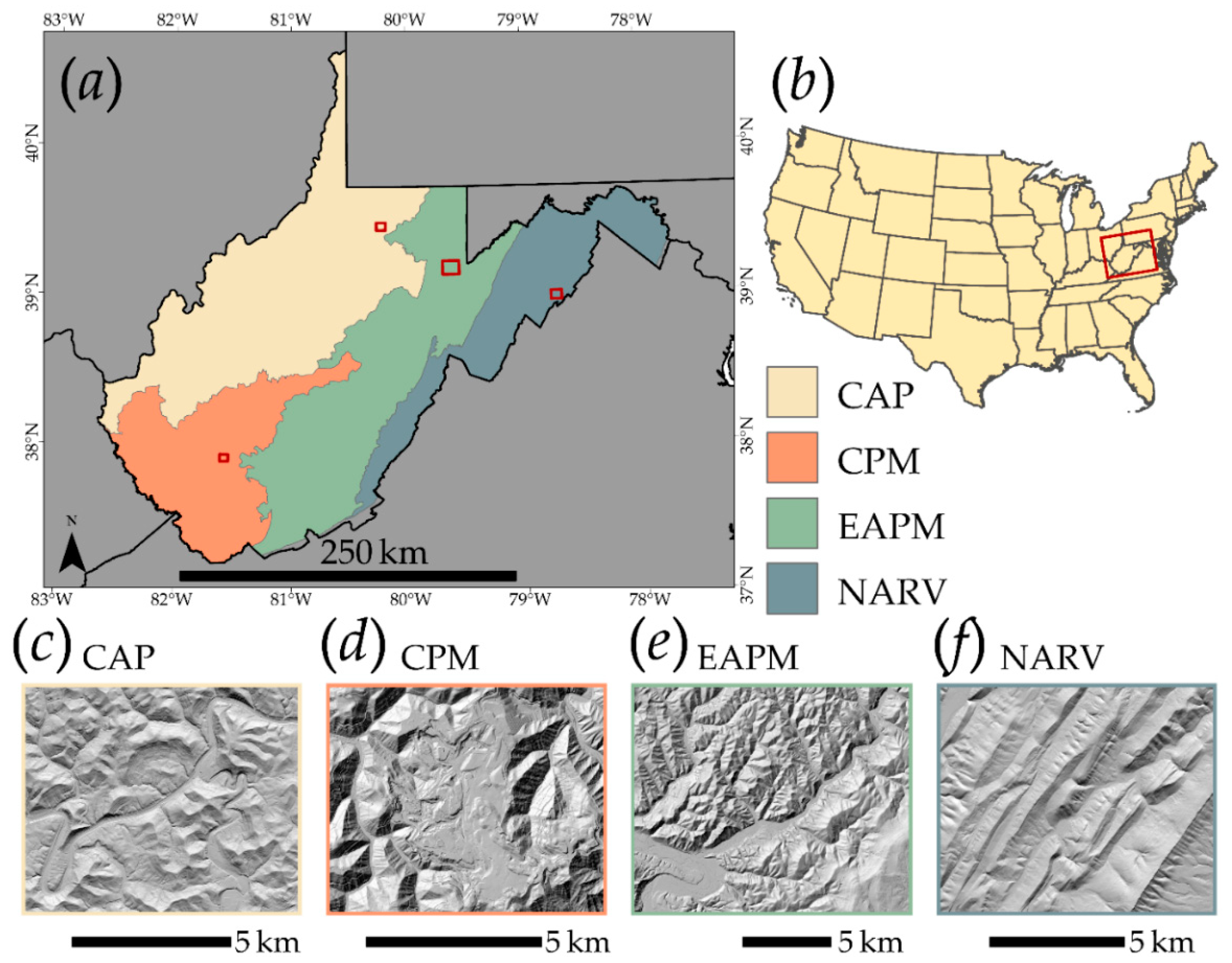
Four separate study areas are investigated, all within the state of West Virginia in the United States. These study areas are defined by Major Land Resource Areas [62] (MLRAs) that intersect West Virginia including the Central Allegheny Plateau (CAP), Cumberland Plateau and Mountains (CPM), Eastern Allegheny Plateau and Mountains (EAPM), and Northern Appalachian Ridges and Valleys (NARV) (Figure 2). Due to varying topography, anthropogenic alterations, disturbance histories, and slope failure presentation, the four MLRAs were treated as separate study areas as opposed to combining the data to generate a single dataset and model.

Figure 2 shows the extent of each MLRA in the state and also provides examples of characteristic surface morphologies using LiDAR-derived hillshades. Generally, the state of West Virginia has a high degree of susceptibility to slope failures due to local relief and steep slopes, a humid climate, weak geologic units, recent stream incision, and anthropogenic landscape modifications [63]. The state experiences average winter temperatures of approximately 0 °C and average summer temperatures of approximately 22 °C, with the lowest seasonal temperatures occurring in the EAPM MLRA. Precipitation is variable resulting from topographic and rain shadow effects. Western-facing slopes in the EAPM generally experience the most precipitation with totals as high as 1600 mm per year while the NARV experiences the lowest, with totals of approximately 635 mm per year. Topography between the MLRAs also varies. For example, the CAP is characterized by a high degree of local relief due to dissection of the plateau by a dendritic stream network while the NARV is characterized by long, linear ridges and valleys resulting from erosion, underlying geologic structure (i.e., synclines and anticlines), and a trellis stream network [64,65]. The steepest slopes generally occur in the CPM, a landscape that has been extensively modified by historic surface coal mining and more recent mountaintop removal coal mining [66,67,68]. In regard to land cover and land use, the state is dominated by forests with development, urbanization, and agriculture concentrated in river valleys [64].

Table 1. MLRA land areas, abbreviations used in this study, and number of mapped slope failure incidence points. Note that a statewide dataset of incidence points is not yet available since LiDAR data collection is not yet complete.

MLRA	Abbreviation	Land Area in WV	Number of Slope Failures Mapped
Central Allegheny Plateau	CAP	22,281 km2	29,637
Cumberland Plateau and Mountains	CPM	11,644 km2	20,712
Eastern Allegheny Plateau and Mountains	EAPM	18,071 km2	12,518
Northern Appalachian Ridges and Valleys	NARV	10,320 km2	1997

provides the land areas and number of mapped slope failures in each MLRA. Each slope failure was mapped as a point feature at the interpreted initiation location or head scarp as opposed to an areal extent due to the large spatial extent to inventory and number of features to be mapped along with the difficulty of accurately and consistently digitizing the full spatial extent of material displacement. Although the lack of slope failure polygons was a limitation in this study, generating an accurate and large dataset of slope failure areal extents across the state was not feasible, and prior studies have successfully used point-based representations of slope failures to train empirical models (e.g., [35,36,37,46]). To date, a total of 64,864 slope failure points has been identified by trained analysts supervised by a professional geomorphologist. The analysts used a combination of post-failure LiDAR-derived hillshades and slopeshades along with ancillary geospatial data to interpret initiation locations. It should be noted that a full inventory for the entire state extent is still pending since a full LiDAR dataset is not yet available. Specifically, full coverages for the CAP, CPM, and EAPM have yet to be made available; however, it is anticipated that these data will be available and post-processed by early 2022. Only areas with LiDAR data available were used. In this study, we do not differentiate types of slides. However, analysts labeled all digitized slope failures as either slides, debris flows, lateral spread, or multiple failures, with the majority categorized as slides. Slope failure incidence points are viewable at the WV Landslide Tool web application (https://www.mapwv.gov/landslide, accessed on 7 December 2021).

3.2. Training Data and Predictor Variables

All algorithms investigated require both presence and absence data. As a result, pseudo absence data were generated as random points within each MLRA. From the set of random points, samples were removed if they (1) did not occur within areas where LiDAR data were available, (2) were within 30 m of a mapped landslide, and/or (3) occurred within the extent of or within 30 m of historic slope failure data provided by the West Virginia Department of Transportation (WVDOT) and the West Virginia Geological and Economic Survey (WVGES). Although historic data were used to refine the pseudo absence data, these data were not used to train or validate the resulting models. Instead, we only relied on the point features that were manually interpreted for consistency. This was the same pseudo absence sampling method used in our prior studies in the series [8,9].

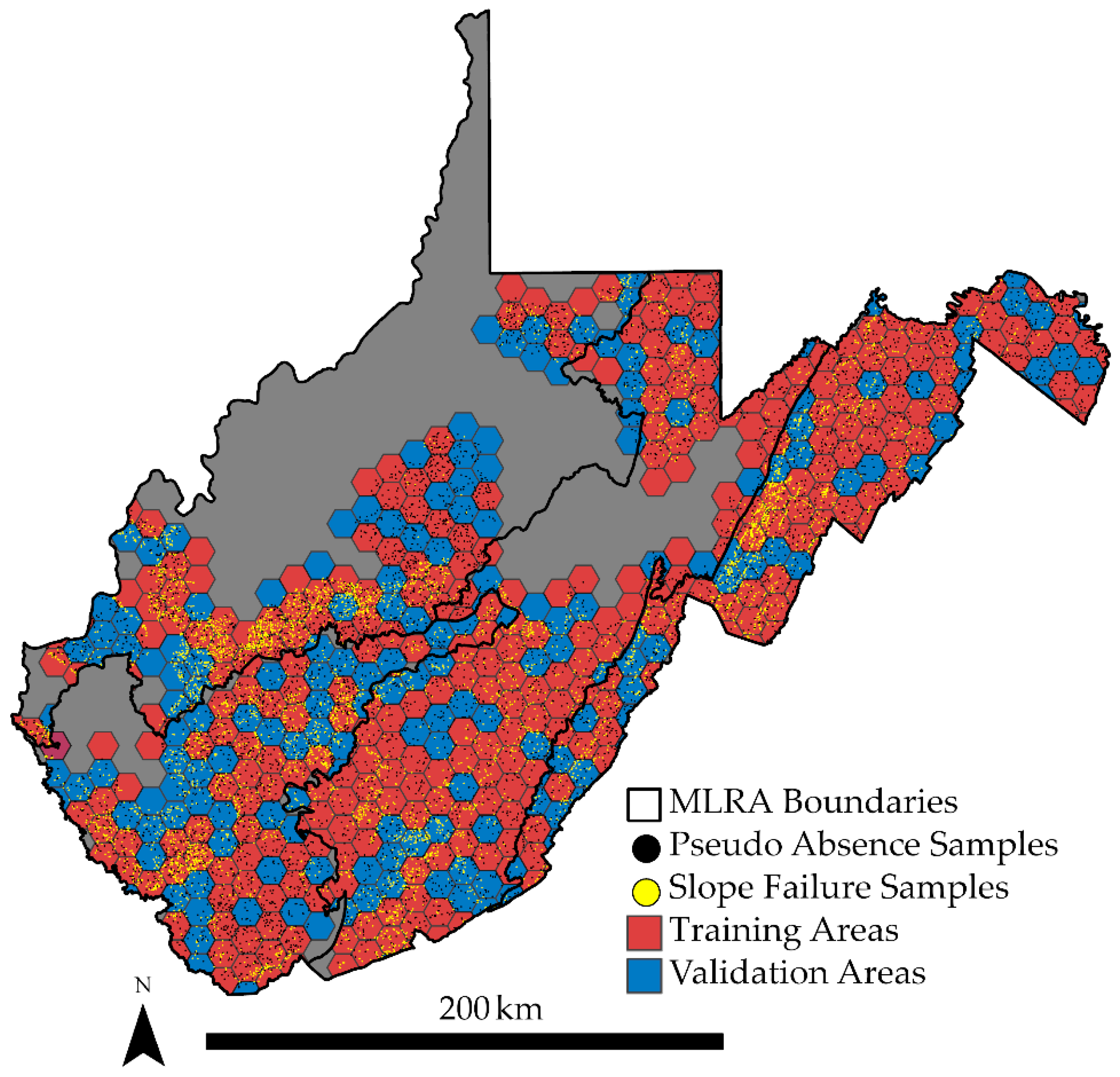
In order to perform consistent experimentation across the four different MLRAs and the different algorithms, we randomly selected 1200 slope failure and 1200 pseudo absence samples, or 2400 samples in total, from the complete dataset available for each MLRA. For model validation, 500 slope failure and pseudo absence samples, or a total of 1000 samples, were randomly selected such that the training and validation sets were non-overlapping. Further, in order to reduce spatial autocorrelation between the training and validation samples, which may optimistically bias the assessment, each MLRA was tessellated into 10,000-hectare contiguous hexagons (Figure 3). Random training and validation partitioning were conducted to ensure that slope failure and pseudo absence samples within the same hexagon bin occurred in the same split and also could not be included in both the training and validation partitions. In summary, in order to foster a fair comparison between different MLRAs, we used the same number of training samples. For a fair comparison between algorithms, each algorithm within each MLRA was trained and validated using the same sample partitions.

In order to assess how the algorithms respond to a reduction in the number of training features, we also randomly extracted samples from the full 2400 training point datasets in each MLRA. We generated training sets with 10, 50, 100, 200, 300, 400, 500, 600, 700, 800, 900, 1000, and 1100 samples per class. The same samples selected in each set were used to train all the algorithms to ensure a fair comparison between methods.

Additionally, for consistency and because our prior study [8] documented only marginal improvements when non-terrain predictor variables were included in the feature space, in this study, we only used terrain variables that could be consistently generated from the post-failure LiDAR-derived DTM for all MLRAs. The calculated variables are summarized in

Table 2. Description of terrain variables used in this study. Abbreviations defined in this table are used throughout this paper.

Variable	Abbreviation	Description	Window Radius (Cells)
Slope Gradient	Slp	Gradient or rate of maximum change in Z as degrees of rise	1
Mean Slope Gradient	SlpMn	Slope averaged over a local window	7, 11, 21
Linear Aspect	LnAsp	Transform of topographic aspect to linear variable	1
Profile Curvature	PrC	Curvature parallel to direction of maximum slope	7, 11, 21
Plan Curvature	PlC	Curvature perpendicular to direction of maximum slope	7, 11, 21
Longitudinal Curvature	LnC	Profile curvature intersecting with the plane defined by the surface normal and maximum gradient direction	7, 11, 21
Cross-Sectional Curvature	CSC	Tangential curvature intersecting with the plane defined by the surface normal and a tangent to the contour—perpendicular to maximum gradient direction	7, 11, 21
Slope Position	TPI	Z–Mean Z	7, 11, 21
Topographic Roughness	TRI	Square root of standard deviation of slope in local window	7, 11, 21
Topographic Dissection Index	TDI	$\frac{\mathrm{Z}-Min Z}{Max Z-Min Z}$	7, 11, 21
Surface Area Ratio	SAR	$\frac{Cell Area}{\mathrm{cosine} \left(slope \ast \pi \ast 180\right)}$	1
Surface Relief Ratio	SRR	$\frac{Mean \mathrm{Z}-Min Z}{Max Z-Min Z}$	7, 11, 21
Site Exposure Index	SEI	Measure of exposure based on slope and aspect	1
Heat Load Index	HLI	Measure of solar insolation based on slope, aspect, and latitude	1

. These variables were selected to capture a wide range of local topographic characteristics relating to steepness, curvature, orientation, slope position, rugosity, incision, and incoming solar radiation. All variables were calculated from the 2 m spatial resolution, LiDAR-derived DTM. Any variable that required defining a local moving window was calculated using multiple window sizes (i.e., circular windows with radii of 7, 11, and 21 cells) in order to capture terrain characteristics at varying spatial scales. Scales were selected based on common ridge-to-valley distances across the study area extents.

Based on a principal component analysis, 95% of the total variance in all 32 included predictor variables was explained with 12 or 13 principal components. The mean absolute Spearman’s rank correlation coefficient for variable pairs were 0.31, 0.28, 0.33, and 0.31 for the CAP, CPM, EAPM, and NARV MLRAs, respectively. Of all possible predictor variable pairs (496), the number that had a Spearman’s rank correlation coefficient larger than 0.90 were 18, 17, 28, and 32 for the CAP, CPM, EAPM, and NARV MLRAs, respectively. In summary, there is some multi-collinearity between the provided terrain predictor variables. This was especially true when the same variable was calculated using different moving window sizes.

Slope gradient (Slp) [69] was calculated using the Slope Tool made available in the Spatial Analyst Extension of ArcGIS Pro [70]. The Geomorphometry and Gradient Metrics Toolbox [71] extension for ArcGIS Pro was used to calculate mean slope gradient (SlpMn) [69], linear aspect (LnAsp) [72], the topographic position index (TPI) [73], the topographic roughness index (TRI) [74,75], the topographic dissection index (TDI) [76], the surface area ratio (SAR) [77], the surface relief ratio (SRR) [78], the site exposure index (SEI) [79], and the heat load index (HLI) [80]. Profile (PrC), plan (PlC), longitudinal (LnC), and cross-sectional (CSC) curvatures [81,82] were calculated using the Morphometric Features Module in the open-source System for Automated Geoscientific Analysis (SAGA) software [83,84]. A total of 32 topographic predictor variables were used. All raster grid cell values at the training and validation sample point locations were then extracted without bilinear interpolation to generate tables using the Extract Multi Values to Points tool in ArcGIS Pro [70].

3.3. Model Traning

The kNN, LR, RF, and SVM algorithms were trained using the caret [85] package in R [86]. This package acts as a wrapper that allows for the execution of a variety of ML methods using consistent syntax. The kNN algorithm uses the class package [87] while LR uses stats [86], RF uses randomForest [88], and SVM uses kernlab [89]. LR was implemented without hyperparameter optimization while kNN, RF, and SVM were optimized using five-fold cross validation. In order to avoid model bias, the cross-validation only used samples from the training set that occurred within the randomly selected hexagonal tessellation units. The validation samples were not used to optimize the models. Each model was trained five times, using four of the folds and maintaining the final fold for performance assessment. Once all folds were withheld, results were average to obtain final assessment metrics for each hyperparameter combination tested. A total of 20 values were tested for all optimized hyperparameters. For the number of neighbors (k) parameter for kNN, values between 5 and 43 were tested while values between 2 and 32 were tested for the RF number of variables available for splitting at each node (mtry) parameter. The cost parameter (c) was optimized for SVM, and values between roughly 1e-1 and 1e5 were tested. For RF, 501 trees were used in all models. SVM made use of a radial basis function (RBF). The best average AUC ROC for the withheld folds was used to select the final hyperparameters and train the final model.

EBM was implemented using Python [90] and the InterpretML library [91]. Default parameters were used, as suggested by the library originators [6,11] and also to specifically assess how well the algorithm performed “out-of-box”. Specifically, 5000 rounds of boosting were used with a learning rate of 0.01. We obtained all graphics representing the one-dimensional feature functions for each predictor variable, two-dimensional feature functions for included interactions, and global importance estimates based on mean absolute scores. We also explored local predictions for selected points.

3.4. Model Assessment

In order to assess model generalization to new geographic extents, all trained models were applied to the validation data in the MLRAs in which they were trained and also all other MLRAs. Several binary, threshold-based metrics were calculated including overall accuracy (OA) and precision, recall, F1 score, sensitivity, and negative predictive value (NPV) with the slope failure class as the positive case. Samples with a predicted probability of occurrence in the slope failure class of greater than or equal to 0.5 were classified to the positive case while those lower than 0.5 were mapped to the negative case.

Table 3. Example binary confusion matrix and associated terminology. TP = true positive, FP = false positive, TN = true negative, and FN = false negative.

		Reference Data
		True	False	1—Commission Error
Classification Result	True	TP	FP	Precision
	False	FN	TN	NPV
	1—Omission Errors	Recall	Specificity

provides the terminology used to define the calculated metrics. True positive (TP) samples are those that are in the slope failure class and are correctly mapped as failures while false positives (FPs) are not in the slope failure class (i.e., pseudo absence samples) but are incorrectly mapped as failures. True negatives (TNs) are pseudo absence samples correctly mapped as not failures while false negatives (FNs) are mapped as not failures when they are actually failures.

Overall accuracy (OA) (Equation (3)) represents the proportion of correctly classified samples in both classes. Precision (Equation (4)) is equivalent to 1—commission error while recall or sensitivity (Equation (5)) represents 1—omission error relative to the slope failure class. The F1 score (Equation (6)) is the harmonic mean of precision and recall. Similar to precision and recall, negative predictive value (NPV) (Equation (7)) and specificity (Equation (8)) represent 1—commission error and 1—omission error for the negative or not slope failure class, respectively [92]. All binary assessment metrics were calculated using the caret [85] package in R [86], which allows for the calculation of 95% confidence intervals for OA based on a binomial distribution [85,93].

$$\mathrm{Overall} \mathrm{Accuracy} (\mathrm{OA})=\frac{\mathrm{TP}+\mathrm{FP}}{\mathrm{TP}+\mathrm{TN}+\mathrm{FP}+\mathrm{FN}}$$

(3)

$$\mathrm{Precision}=\frac{\mathrm{TP}}{\mathrm{TP} + \mathrm{FP}}$$

(4)

$$\mathrm{Recall} \mathrm{or} \mathrm{Sensitivity}=\frac{\mathrm{TP}}{\mathrm{TP} + \mathrm{FN}}$$

(5)

$$\mathrm{F}1 \mathrm{Score}=\frac{2\times \mathrm{Precision} \times \mathrm{Recall}}{\mathrm{Precision} + \mathrm{Recall}}$$

(6)

$$\mathrm{Negative} \mathrm{Predictive} \mathrm{Value} (\mathrm{NPV})=\frac{\mathrm{TN}}{\mathrm{TN} + \mathrm{FN}}$$

(7)

$$\mathrm{Specificity}=\frac{\mathrm{TN}}{\mathrm{TN} + \mathrm{FP}}$$

(8)

We also calculated metrics that make use of predicted class probabilities and do not require defining a binary decision threshold. First, we calculated receiver operating characteristic (ROC) curves and the associated area under the curve measure (AUC ROC). An ROC curve plots 1—specificity on the x-axis and sensitivity or recall on the y-axis at varying decision thresholds [92,94,95,96]. The AUC ROC measure is the area under the ROC curve and is scaled from 0 to 1, with larger values indicating better model performance [92,94,95,96,97]. This analysis was undertaken using the pROC package [97] in R [86], which allows for the estimation of 95% confidence intervals for AUC ROC.

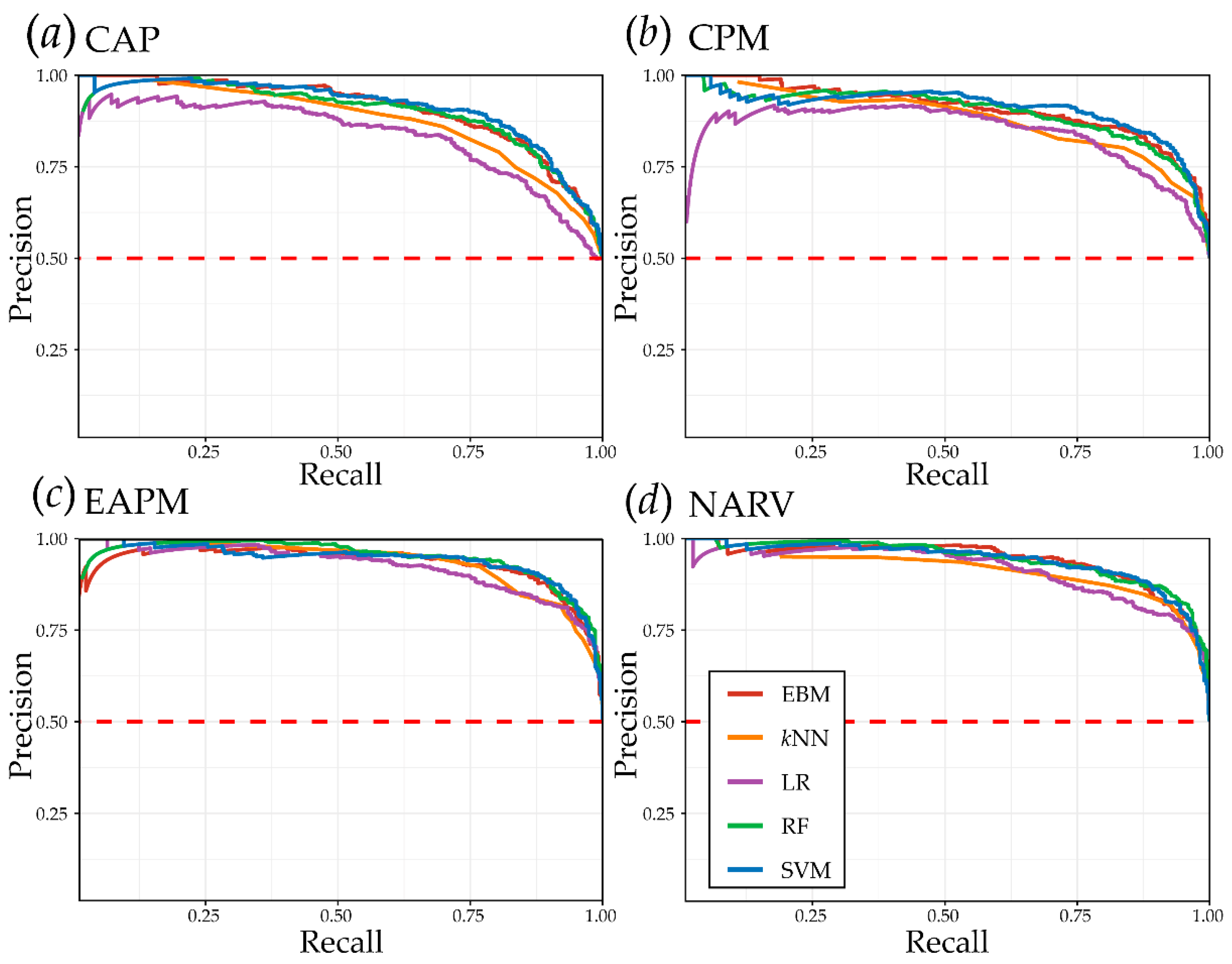
Since ROC curves and the associated AUC ROC metric rely on recall and specificity, both measures of 1—omission error, and do not take into account precision, or 1—commission error relative to the positive case [92,98], we also calculated precision-recall (P-R) curves, which consider recall and precision, or 1—omission and 1—commission error relative to the positive case. This curve plots recall to the x-axis and precision to the y-axis. Similar to ROC curves, an area under the curve (AUC PR) metric can be calculated to obtain a single summary statistic [92,98,99]. This analysis was completed using the yardstick package [100] in R [86].

It should be noted that many assessment metrics are impacted by the relative proportions of classes within the landscape or validation set [92]. Given that slope failure initiation locations make up a small proportion of the landscape and that the actual landscape proportion is not known a priori, it was not possible to assess the model using correct landscape proportions. Instead, we relied on a balanced sample to assess the differentiation of the slope failure class from the background. Since a large portion of the landscape is not a slope failure initiation location, there is a greater chance of FPs than is represented in our validation sample. When class proportions are not known, such as for predicting habitat suitability or future landscape change, it is common to use a class-balanced validation set (for example [101,102,103]).

4. Results

4.1. Algorithm Comparisons

Table 4. Assessment metrics calculated using the withheld validation samples in each MLRA for each algorithm. OA = overall accuracy, NPV = negative predictive value, AUC ROC = area under the receiver operating characteristics curve, and AUC PR = area under the precision-recall curve.

Study Area	Algorithm	OA	Precision	F1 Score	Recall	Specificity	NPV	AUC ROC	AUC PR
CAP	EBM	0.823	0.857	0.814	0.776	0.870	0.795	0.903	0.909
CAP	kNN	0.806	0.834	0.797	0.764	0.848	0.782	0.884	0.888
CAP	LR	0.789	0.819	0.779	0.742	0.836	0.764	0.843	0.844
CAP	RF	0.839	0.854	0.836	0.818	0.860	0.825	0.903	0.905
CAP	SVM	0.854	0.886	0.848	0.812	0.896	0.827	0.911	0.906
CPM	EBM	0.849	0.847	0.849	0.852	0.846	0.851	0.917	0.909
CPM	kNN	0.815	0.801	0.819	0.838	0.792	0.830	0.888	0.880
CPM	LR	0.797	0.799	0.796	0.794	0.800	0.795	0.870	0.839
CPM	RF	0.835	0.829	0.836	0.844	0.826	0.841	0.910	0.899
CPM	SVM	0.857	0.844	0.860	0.876	0.838	0.871	0.924	0.910
EAPM	EBM	0.875	0.854	0.879	0.904	0.846	0.898	0.945	0.930
EAPM	kNN	0.853	0.831	0.858	0.886	0.820	0.878	0.936	0.936
EAPM	LR	0.850	0.830	0.854	0.880	0.820	0.872	0.931	0.923
EAPM	RF	0.877	0.848	0.882	0.918	0.836	0.911	0.955	0.944
EAPM	SVM	0.890	0.878	0.892	0.906	0.874	0.903	0.949	0.942
NARV	EBM	0.870	0.857	0.872	0.888	0.852	0.884	0.947	0.941
NARV	kNN	0.859	0.845	0.862	0.880	0.838	0.875	0.924	0.912
NARV	LR	0.831	0.814	0.835	0.858	0.804	0.850	0.925	0.915
NARV	RF	0.884	0.861	0.888	0.916	0.852	0.910	0.948	0.944
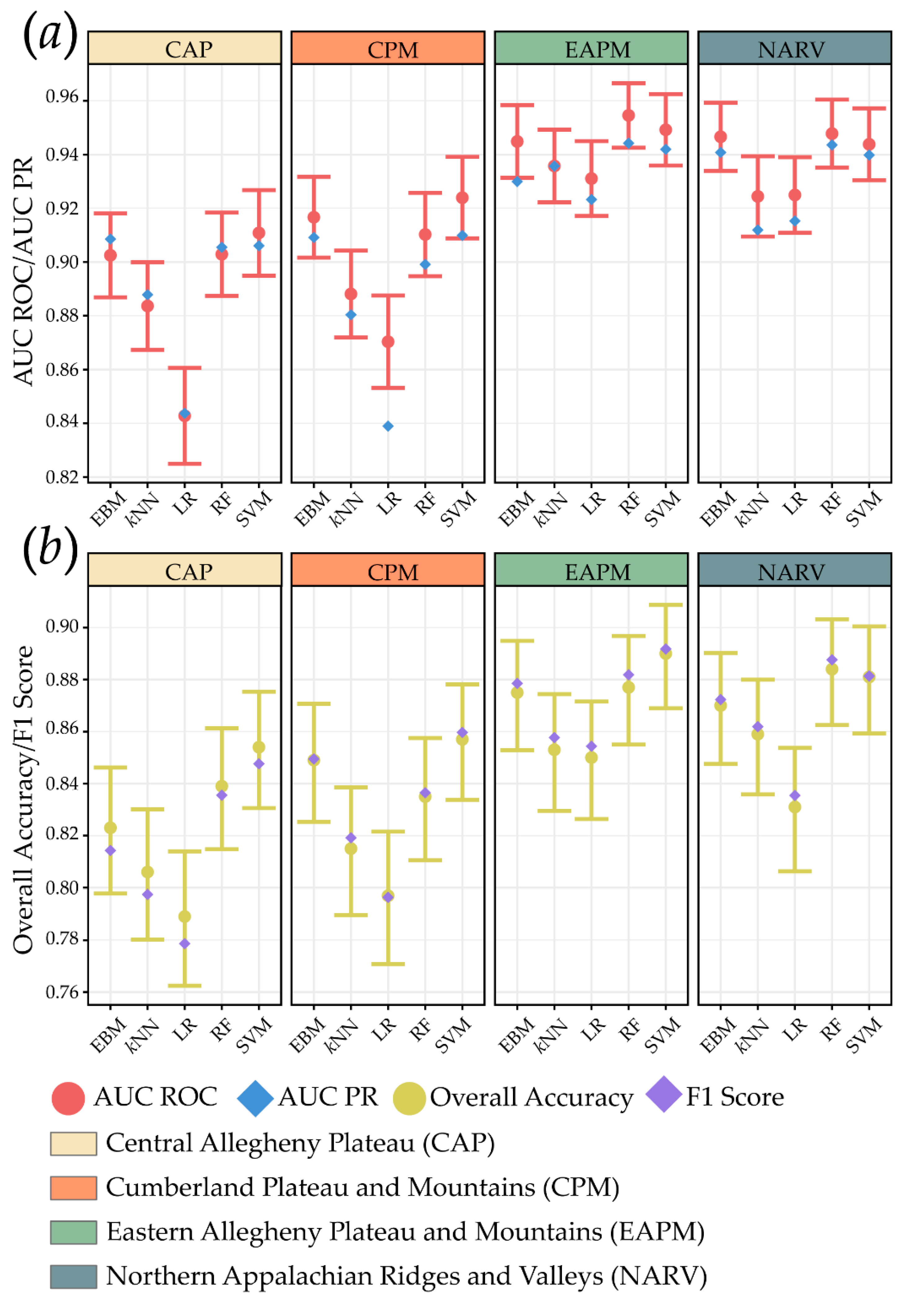
NARV	SVM	0.881	0.879	0.881	0.884	0.878	0.883	0.944	0.940

reports the assessment metrics obtained by predicting to the 1000 withheld validation samples within each MLRA study area using each algorithm while Figure 4 shows the OA, F1 score, AUC ROC, and AUC PR results specifically. Generally, the LR and kNN algorithms showed the weakest performance while the EBM, RF, and SVM algorithms showed the strongest performance. The slope failure predictions for the CAP and CPM regions generally had lower accuracies than those of the EAPM and NARV for all tested algorithms. Additionally, as evident in Figure 4, we observed more disparity in model performance between algorithms in the CAP and CPM in comparison to the EAPM and NARV.

The EBM method provided comparable performance to the current standard black box RF and SVM methods for this specific task. Overall accuracies for predicting slope failure in the CAP, CPM, EAPM, and NARV regions using EBM were 0.823, 0.849, 0.875, and 0.870, respectively, while F1 scores for the slope failure class were 0.814, 0.849, 0.879, and 0.872. AUC ROC and AUC PR values were all above 0.900 for all MLRAs when predicted using EBM.

The ROC and PR curves shown in Figure 5 and Figure 6, respectively, support the results highlighted in Table 4 and Figure 5. EBM generally performed comparably to RF and SVM while outperforming kNN and LR. The CAP and CPM MLRAs were generally predicted with lower accuracies than the EAPM and NARV regardless of the algorithm used. Additionally, there was generally more variability in performance between algorithms in the CAP and CPM. EBM, similar to RF and SVM, showed strong performance across a wide variety of decision thresholds. Additionally, sources of error varied between the different MLRAs when predicted using EBM since, amongst the precision, recall, specificity, and NPV metrics, no measure was consistently higher or lower than the others across all MLRAs. The strength of the ROC and PR curves is that they illustrate the trade-offs associated with predicting slope failure. The likelihood of slope failure is not a binary variable, but instead is a fuzzy variable. Figure 5a shows that in the CAP, LR and kNN underperform the other methods, irrespective of the threshold for labeling a pixel likely to experience slope failure. In contrast, in the EAPM (Figure 6c), the different methods are similar across most thresholds, and the lower performance of LR and kNN is associated with just part of the graph.

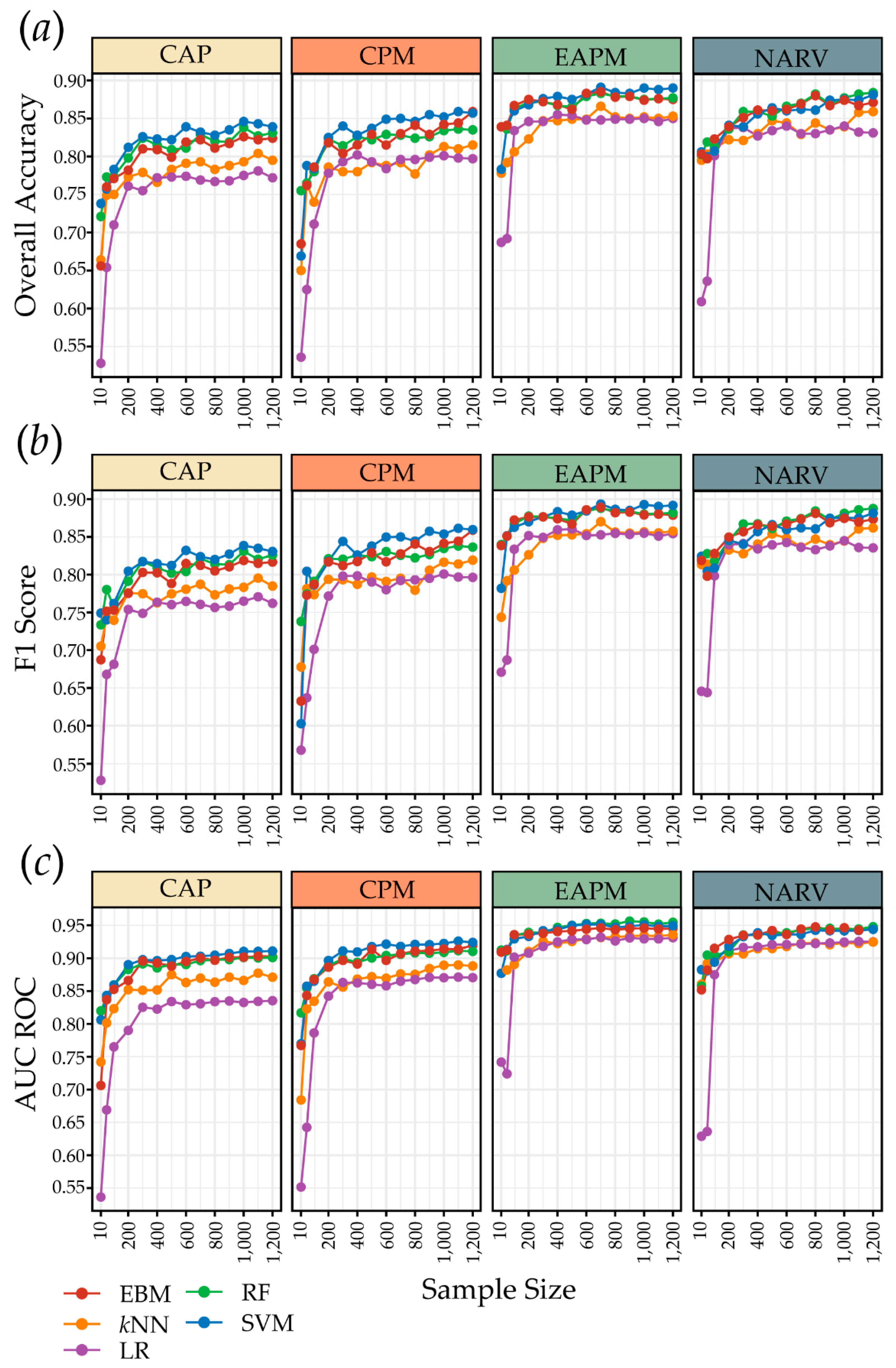
4.2. Sample Size and Model Generalization

Figure 7 summarizes for each MLRA how all tested algorithms responded to a reduction in the number of training samples from 1200 samples per class to just 10. Similar to the overall accuracy results discussed above, EBM performed similarly to RF and SVM in regard to predictive performance as measured with OA, F1 score, and AUC ROC. The sample size experimentation confirms that this pattern holds across a range of sample sizes: EBM, RF, and SVM outperformed kNN and LR regardless of sample size. The study areas that were predicted with higher accuracies generally showed less variability between algorithms while those predicted with lower accuracies showed more variability. Regardless of the algorithm used, predictions for the EAPM MLRA, and to a lesser extent the NARV, generally stabilized or stopped improving when the sample size reached roughly 200 samples per class. For the other areas, performance continued to improve with sample size increases; however, improvements were slow after 200 to 300 samples per class.

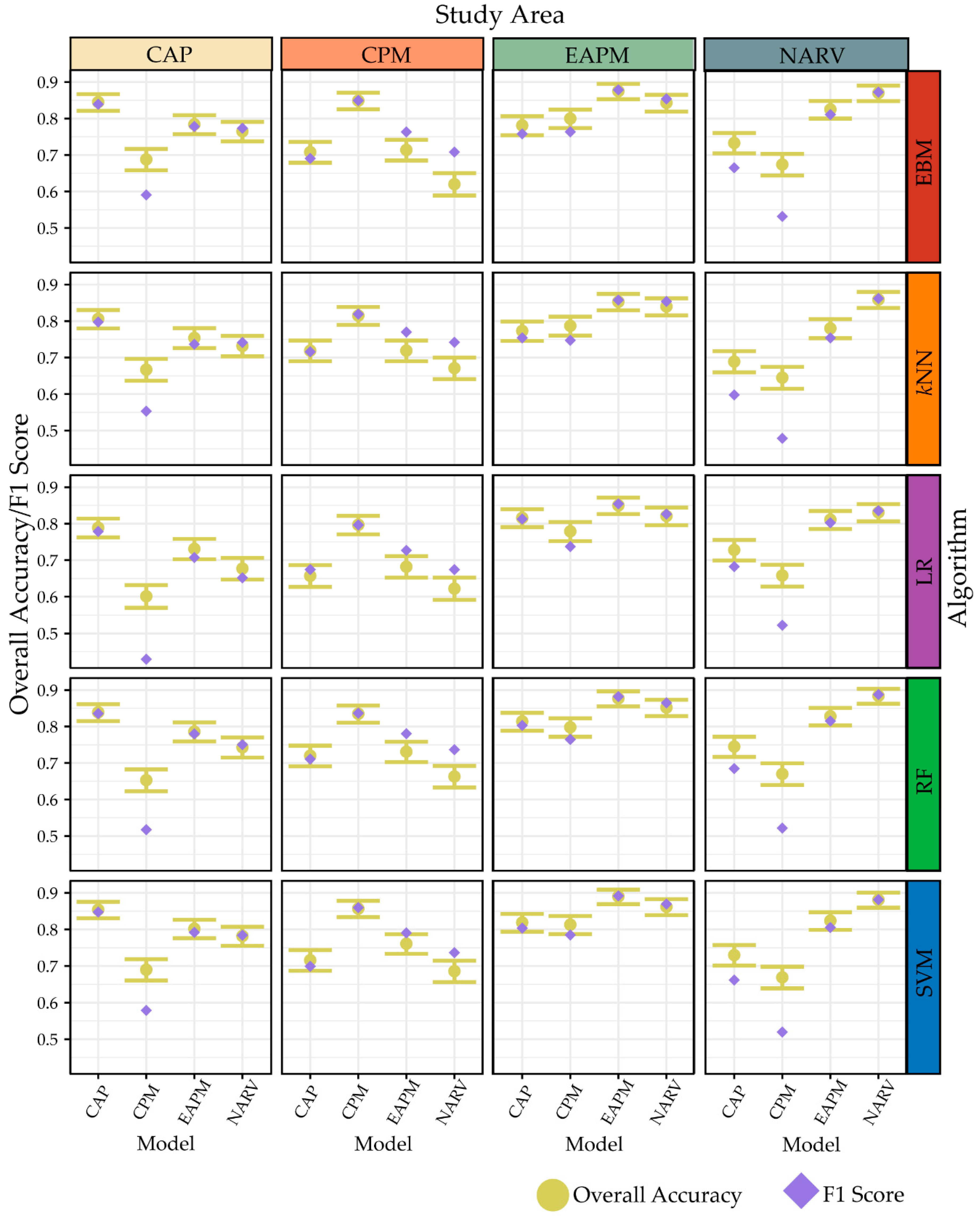
Figure 8 shows the OA and F1 scores obtained when each model was used to predict the validation data within all MLRAs. Similar to the results from our prior study [9], reduced accuracy was observed when trained models were extrapolated to a new MLRA. Expanding upon our prior study, in which only the RF algorithm was assessed, this pattern was observed for all tested algorithms, including EBM. All algorithms provided more similar performance when predicting to the validation data in the EAPM and NARV MLRAs and more disparate performance when predicting to the CAP and CPM. In summary, EBM showed similar generalization trends in comparison to the other tested algorithms.

4.3. Exploration of EBM Results

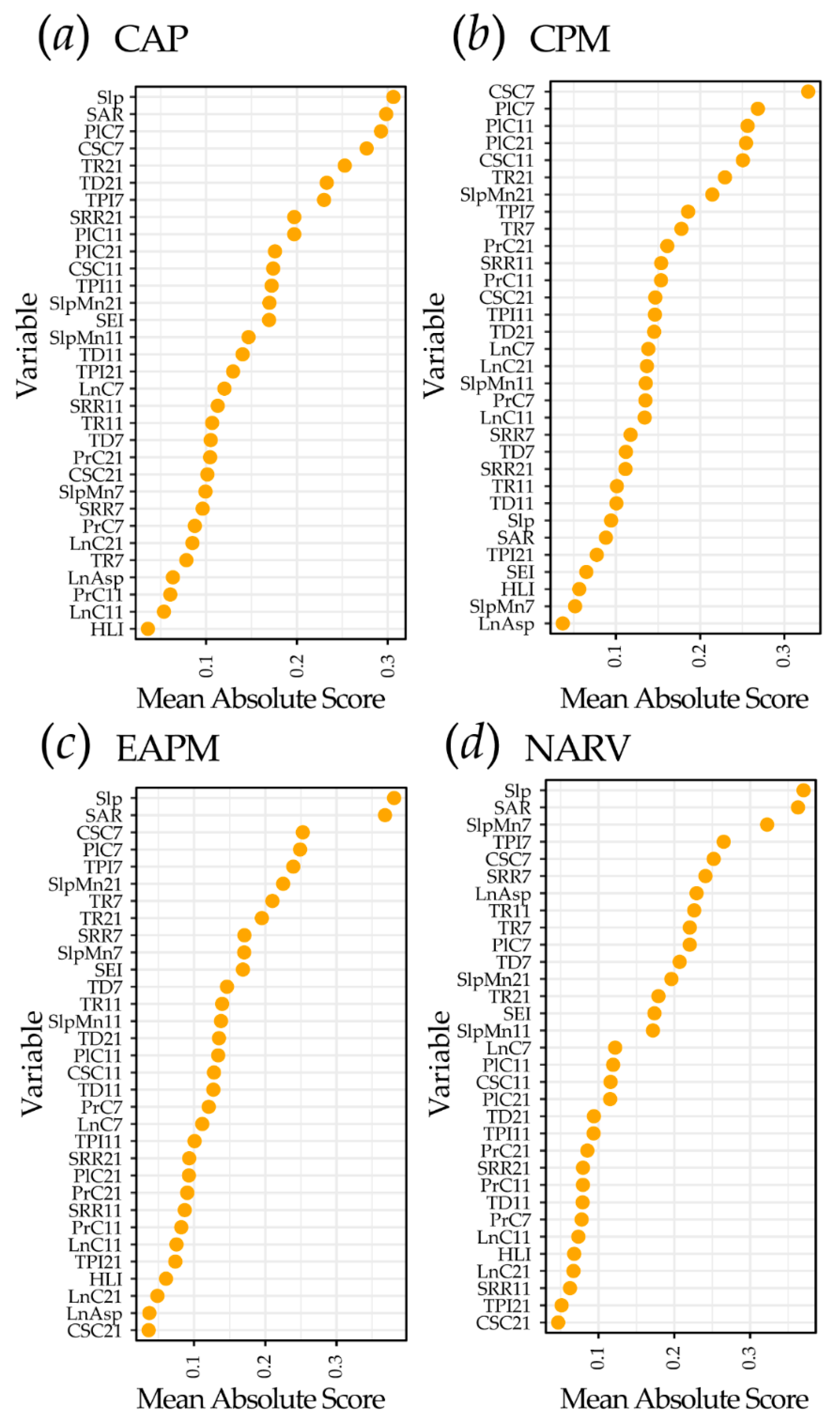
Figure 9 shows variable importance estimates for all terrain predictor variables within each MLRA as estimated using EBM and the mean absolute score metric. Slp was generally found to be important along with SAR, both of which are associated with local topographic steepness. However, the CPM MLRA showed lower importance for Slp and SAR in comparison to the other MLRAs. Generally, variables calculated using a smaller moving window size were more important than the same variable calculated at a larger window size. Some variables were also consistently of low importance, such as LnASP and HLI. This suggests that the orientation of the slope and the amount of incoming solar radiation were not strong predictor variables for estimating slope failure occurrence. In contrast, measures of steepness, roughness, incision, and surface curvature were generally more important.

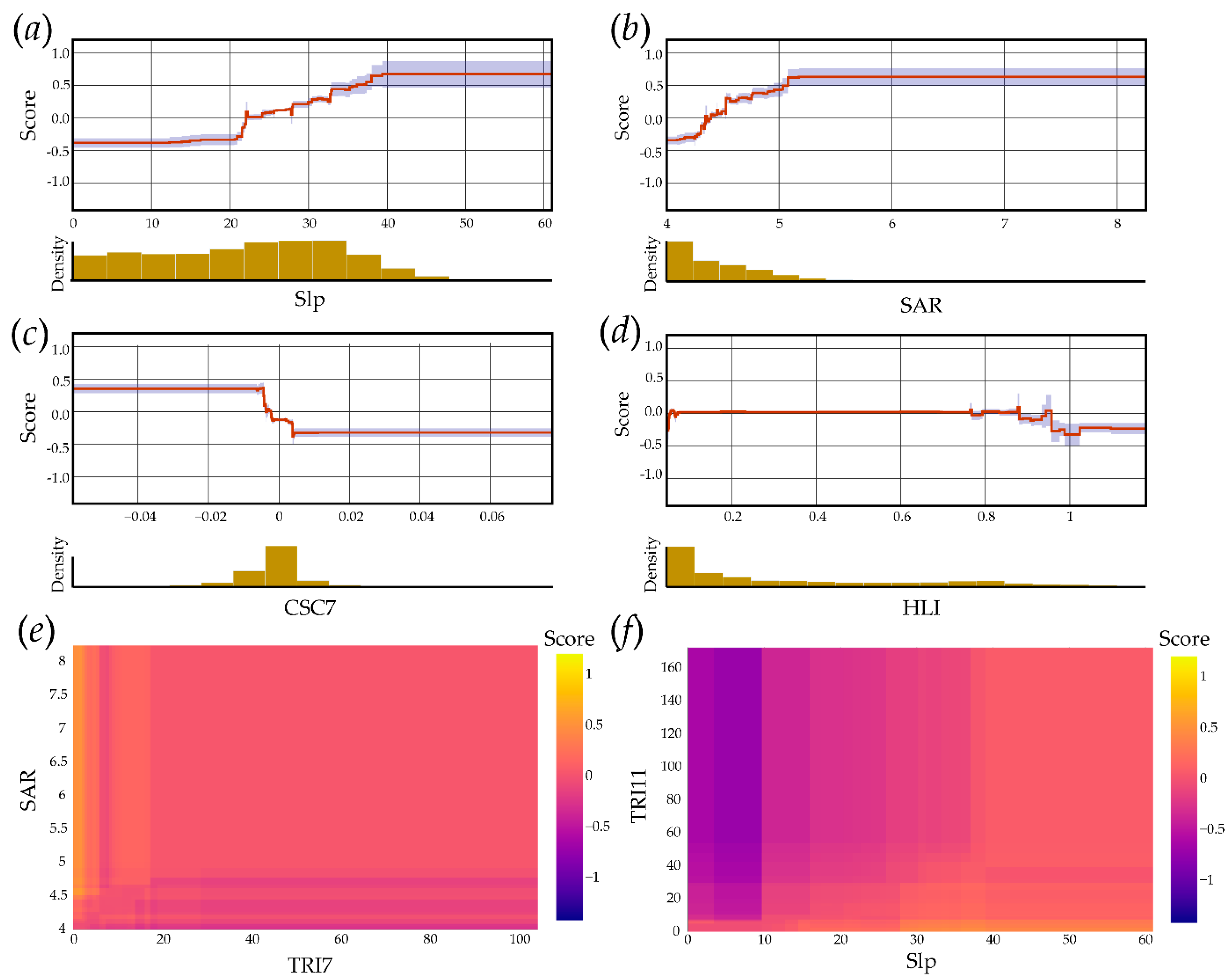
Figure 10 shows some example, ancillary output provided by a trained EBM model for interpreting the global results for the NARV MLRA specifically. As described above, the gradient boosting process results in many decision trees for each predictor variable that are then used to generate the function that describes how the dependent variable, in this case slope failure occurrence, responds to the specific predictor variable [6,7,11]. These functions can then be visualized graphically as a one-dimensional function where the predictor variable values are mapped to the x-axis and the resulting scores (i.e., the effect of the predictor variable on the predicted logits for the positive class) are mapped to the y-axis. Larger scores indicate that predictor variable values in that range are associated with slope failure. Figure 10a–d provide example functions for the Slp, SAR, CSC7, and HLI predictor variables. Again, each predictor variable in the model will have a unique function, which can be visualized graphically to enhance interpretability [6,7].

Figure 10a suggests that slope failures are associated with steeper slopes (Slp) while Figure 11b suggests they are associated with higher surface area ratios (SAR). In contrast, slope failures are associated with more negative cross-sectional curvatures (CSC) (Figure 10c). The heat load index (HLI) (Figure 10d) was a weak predictor variable in each MLRA, including the NARV, based on the importance results discussed above (see Figure 9). As evident in the function, there is little variability in the slope failure occurrence prediction with changes in the HLI.

Pair-wise interactions, for which inclusion has been shown to improve the accuracy of the prediction in comparison to traditional GAMs [7], are described in Figure 10e,f for two example variable pairs. Again, similar graphics are produced for each included pair-wise interaction [6,7]. The graphs indicate that high SAR and low TRI7 values and, similarly, high Slp and low TRI11 values are associated with high scores (i.e., predictions of slope failure occurrence).

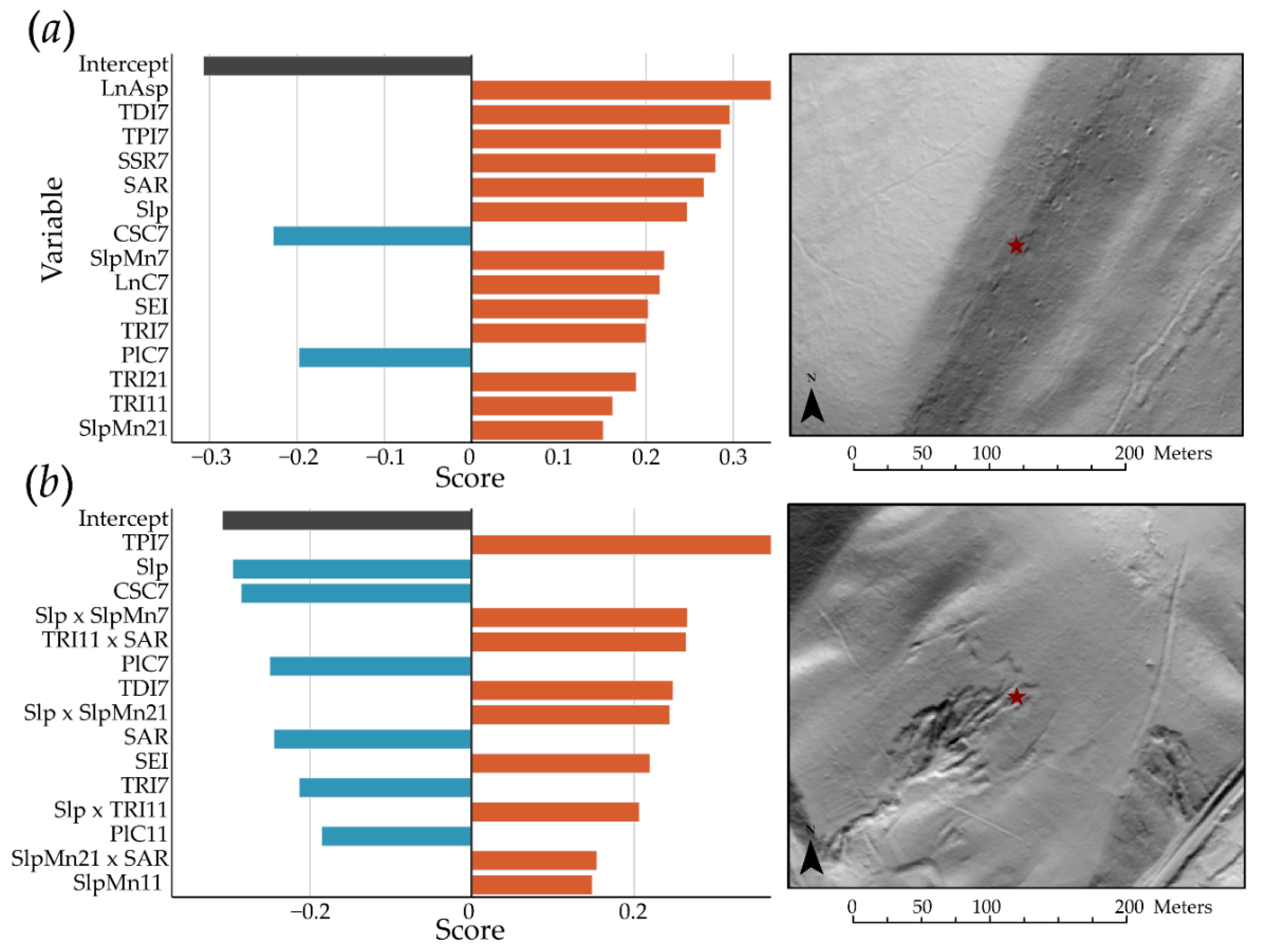
Figure 11 provides variable importance and contribution estimates for predicting two data points within the NARV as an example of local model explanations tied to specific predictions. Again, variable contributions as scores are provided for all predictions to new data [6,7]. The data point presented in Figure 11a is a pseudo absence data point that was incorrectly predicted as a slope failure location with a predicted probability of occurrence of 0.931 while the data point presented in Figure 11b is a slope failure sample that was correctly predicted as a slope failure but with a low probability (0.55). As the results suggest, a variety of site characteristics at the incorrectly predicted pseudo absence point contributed to the results, as many topographic characteristics were indicative of failure. This site is located along a slope break that may result from a rock outcrop or resistant unit. This suggests that the model may predict false positives for rock outcrops that have topographic characteristics similar to slope failure head scarps or initiation locations, on which the model was trained. For example, topographic roughness near this site tended to support the prediction of slope failure occurrence when this characteristic was likely the result of the underly geology and outcropping. These added explanations can highlight some useful limitations or pitfalls for applying and interpreting the model.

In contrast to the incorrectly predicted pseudo absence sample, the low predicted probability of the slope failure point presented in Figure 11b seems to arise from contradictory signals from a variety of terrain variables, as the top contributing variables indicated conflicting scores.

5. Discussion

5.1. Algorithm Performance Comparison and EBM Interpretability

Across the four MLRA study areas, EBM outperformed LR and kNN and performed comparably to RF and SVM for predicting slope failure occurrence based on multiple metrics (i.e., OA, precision, recall, F1 score, specificity, NPV, AUC ROC, and AUC PR). This supports the assertions in the studies that introduced EBM [6,7,11] that the method allows for strong predictive performance. Several prior studies have noted better performance from RF and SVM in comparison to simpler methods, such as kNNs and DTs (e.g., [1,3,104]), for a variety of tasks. For classification tasks in the field of remote sensing, RF and SVM have been suggested as the current standards since they generally outperform the standard and parametric Gaussian maximum likelihood method [1]. Thus, the EBM method provided comparable performance to the current standard black box RF and SVM methods for this specific task.

It should be noted that we did not compare the performance of EBM for this specific task to more traditional GAM methods. Goetz et al. [35] compared many algorithms for slope failure susceptibility modeling, including traditional GAMs, LR, RF, and SVM, and found differences ranging between 2.9 and 8.9 percentage points for the AUC ROC metric. Further, they noted that the RF output, despite strong predictive performance, generated more spatially heterogenous predictions with notable artifacts while GAM, LR, and SVM provided a smoother output [35]. Steger et al. [105] also noted the heterogenous nature of the RF output and further documented that high predictive performance was obtained by a variety of algorithms for landslide susceptibility prediction even though the resulting spatial predictions were inconsistent. Outside of the landslide predictive modeling domain and in the paper that introduced the GA²M method, on which EBM is based, equivalent performance or only marginal improvements in accuracy was noted between GA²M and traditional GAMs, and the major innovation of the method was highlighted as the development of the FAST method for selection of pair-wise interactions to include in the model [7]. More work on relating the predictive performance of EBMs to other GAM-based methods and comparing the spatial outputs, variable importance estimates, feature-specific functions, and two-dimensional interaction heat maps is merited. Further, since EBM relies on shallow decision trees, further investigation is necessary to explore how heterogenous the spatial outputs may be and whether or not artifacts are evident.

Similar to Maxwell et al. [9], in which only the RF algorithm was used, the slope failure predictions for the CAP and CPM regions generally had lower accuracies than those of the EAPM and NARV. Expanding upon this prior study, this trend was consistent for all five tested algorithms. More disparity in model performance between algorithms in the CAP and CPM in comparison to the EAPM and NARV is attributed to a less clear topographic signature for slope failures in these landscapes. For example, the CPM has experienced significant landscape disturbance, alteration, and recontouring as a result of historic surface coal mining and more recent mountaintop removal coal mining [66,67,106], resulting in a very complex topographic surface in which the signature of failures may be less pronounced or unique. Additionally, the EBM-based variable importance estimates suggested that the Slp and SAR variables were less important in this MLRA in comparison to the other three study areas (see Figure 9), which may result from varying landscape conditions and anthropogenic landscape changes. Visual inspection of slope failure locations in the CPM suggests association with mining and mine reclamation, as failures are common around the periphery of reclaimed surface mine sites.

In regard to number of training samples, this study suggests that a large number of samples may not be necessary to obtain accurate results for this specific problem, which supports prior findings from Maxwell et al. [8]. In comparison to RF and SVM, EBM showed similar trends and accuracies as sample size was decreased. This suggest that comparable performance can be obtained when using the EBM method as opposed to RF or SVM regardless of sample size.

All five tested algorithms generally showed reduced performance when used to predict validation data from a different MLRA as opposed to the one in which they were trained. Or, the models did not generalize well to new landscapes with different terrain conditions and disturbance patterns, even though all tested landscapes where within the state of West Virginia, USA. Generally, our results suggest that geographic generalization of EBM models are similar to RF and SVM models for this specific task and investigated landscape.

Our results highlight the interpretability of EBM models and support the assertions of the algorithms developers. Each predictor variable has an associated one-dimensional function that can be visualized graphically. Similarly, each included interaction term can be visualized as a two-dimensional heat map. From these graphics, it is possible to determine the resulting score given any input value. Global interpretability is enhanced by the estimation of variable importance based on the mean absolute score. For each prediction, variable contribution and scores are provided, which helps explain predictions made at all sample points or new locations. This is valuable for determining what site characteristics resulted in the prediction. In summary, for this specific empirical modeling task, EBM offered accuracies comparable to RF and SVM alongside more interpretable results that can be easily visualized graphically.

We also argue that the provided global and local interpretations offer insight for understanding the geologic and surficial conditions that are associated with slope failure occurrence within specific physiographies or at specific locations, respectively. For example, a steeper Slp and higher SAR where generally predictive of slope failure occurrence, which is likely a result of correlation with gravitational potential energy and the presence of slope breaks, such as those associated with a head scarp. This could also be associated with the occurrence of unit contacts where landslides may result from a resistant unit positioned above a less resistant unit that has been eroded. In the NARV specifically, there are many geologic contacts occurring at often steep dip angles due to significant geologic folding [64,65]. As noted above, Slp and SAR were generally less predictive of landslide occurrence in the CPM MLRA, which we attribute to anthropogenic landscape alterations and a naturally steep topography where steepness may be of less use for differentiating failures from other landscape features. Surface roughness was also generally correlated with slope failure occurrence, which could result from the irregular topography associated with failures (e.g., minor scarps and transverse cracks) and displaced debris or talus. It should be noted that the inclusion of a large number of correlated variables increases the complexity of assessing the correlation between each predictor variable and the likelihood of slope failure occurrence. As discussed below, implementing an interpretable model has additional implications for selecting predictor variables to include in the feature space. Interpretation is especially difficult when the same variable is calculated using different moving window sizes to characterize landscape patterns at varying scales. This highlights the need to investigate alternative methods to either select appropriate window sizes or summarize the landscape at multiple scales using a smaller set of variables.

5.2. Future Research Needs

Since EBM can be used for regression, binary classification, multiclass classification, and probabilistic modeling, it has many potential applications in spatial predictive mapping and modeling and remote sensing (e.g., forest biomass estimation, soil properties prediction, land cover classification, landform mapping, and species habitat prediction). Given that the EBM classification performance documented here was comparable to RF and SVM, the current standards in remote sensing, additional research on this algorithm is merited. Exploration of how EBM-based predictions are impacted by imbalance in training data would be useful. It would also be useful to further investigate how the inclusion of interaction terms may impact model interpretability and, specifically, the contribution of specific variables. Further exploration is required to better understand the impact on accuracy and interpretability of including a large number of correlated predictor variables. The importance estimation based on the mean absolute score needs to be further explored. For example, many studies have investigated the permutation-based variable importance measures generated by RF and have noted issues when variables are highly correlated and/or measured on different scales. Issues also arise when a mix of categorical and continuous predictor variables are included and/or when categorical variables have varying numbers of levels. This has led to the augmentation of the RF variable importance methods for addressing these issues and specifically obtaining estimates of marginal vs. partial variable importance (see, for example, [17,18,107]). If EBM-based variable importance estimates are to be adopted more widely, similar investigations, and potentially refinements and augmentations, are necessary.

If it is decided that model interpretability is of importance, this may impact other modeling decisions as opposed to just the algorithm used. For example, including a large number of predictor variables that are not well understood by the end user would still hinder interpretation. In this study, a large number of predictor variables were used, some of which may not be easy to interpret or could result from differing causes or be associated with varying landscape characteristics. Thus, the end user would need to have an understanding of the terrain variables used, how they were calculated, and what site characteristics they correlate with in order to make full use of the global and local interpretations. Additionally, the reported accuracies, estimated predictor variable functions, and variable importance estimates may not be consistent across disparate landscapes or when using input terrain data of varying spatial resolutions. To make use of the local interpretations specifically, resulting models would need to be presented in a manner that allows access to the ancillary output. For example, it would be valuable to be able to select a raster cell and obtain the local interpretation outputs, as shown in Figure 11 for two sample points, along with the probabilistic prediction.

6. Conclusions

In this study, we have documented that EBMs can offer predictive performance comparable to RF and SVM and stronger performance than simpler methods, such as LR and kNN, while also providing model interpretability by the generation of global explanations consisting of graphics representing the functions associated with each predictor variable, heat maps associated with each included pair-wise interaction, and estimates of variable importance based on mean absolute score. Local interpretations are provided for all new predictions that summarize the scores associated with each predictor variable or included pair-wise interaction. Since being able to understand the global model, the contributions of specific predictor variables, the model response to specific predictor variables, and why certain samples or locations were predicted to have high or low likelihood of slope failure occurrence can be of great value, we argue that the EBM algorithm should be further investigated as a tool for geohazard predictive modeling. More generally, this method should be further explored for additional tasks in spatial predictive modeling and analysis of remotely sensed data.

This study highlights the value of EBM and calls for further exploration of its application and interpretation within geohazard mapping and modeling specifically and spatial predictive mapping and modeling in general, especially when the interpretability of the result is important and not just predictive accuracy.

References

1. Maxwell, A.E.; Warner, T.A.; Fang, F. Implementation of Machine-Learning Classification in Remote Sensing: An Applied Review. Int. J. Remote Sens. 2018, 39, 2784–2817. [Google Scholar] [CrossRef] [Green Version]
2. James, G.; Witten, D.; Hastie, T.; Tibshirani, R. An Introduction to Statistical Learning; Springer: Berlin/Heidelberg, Germany, 2013; Volume 112. [Google Scholar]
3. Mountrakis, G.; Im, J.; Ogole, C. Support Vector Machines in Remote Sensing: A Review. ISPRS J. Photogramm. Remote Sens. 2011, 66, 247–259. [Google Scholar] [CrossRef]
4. Rudin, C. Stop Explaining Black Box Machine Learning Models for High Stakes Decisions and Use Interpretable Models Instead. Nat. Mach. Intell. 2019, 1, 206–215. [Google Scholar] [CrossRef] [Green Version]
5. Papernot, N.; McDaniel, P.; Goodfellow, I.; Jha, S.; Celik, Z.B.; Swami, A. Practical Black-Box Attacks against Machine Learning. In Proceedings of the 2017 ACM on Asia Conference on Computer and Communications Security, Abu Dhabi, United Arab Emirates, 2–6 April 2017; pp. 506–519. [Google Scholar]
6. Nori, H.; Jenkins, S.; Koch, P.; Caruana, R. InterpretML: A Unified Framework for Machine Learning Interpretability. arXiv 2019, arXiv:1909.09223. [Google Scholar]
7. Lou, Y.; Caruana, R.; Gehrke, J.; Hooker, G. Accurate Intelligible Models with Pairwise Interactions. In Proceedings of the 19th ACM SIGKDD International Conference on Knowledge Discovery and Data Mining, Chicago, IL, USA, 11–14 August 2013; pp. 623–631. [Google Scholar]
8. Maxwell, A.E.; Sharma, M.; Kite, J.S.; Donaldson, K.A.; Thompson, J.A.; Bell, M.L.; Maynard, S.M. Slope Failure Prediction Using Random Forest Machine Learning and LiDAR in an Eroded Folded Mountain Belt. Remote Sens. 2020, 12, 486. [Google Scholar] [CrossRef] [Green Version]
9. Maxwell, A.E.; Sharma, M.; Kite, J.S.; Donaldson, K.A.; Maynard, S.M.; Malay, C.M. Assessing the Generalization of Machine Learning-Based Slope Failure Prediction to New Geographic Extents. ISPRS Int. J. Geo. Inf. 2021, 10, 293. [Google Scholar] [CrossRef]
10. Hastie, T.; Tibshirani, R. Generalized Additive Models: Some Applications. J. Am. Stat. Assoc. 1987, 82, 371–386. [Google Scholar] [CrossRef]
11. Nori, H.; Caruana, R.; Bu, Z.; Shen, J.H.; Kulkarni, J. Accuracy, Interpretability, and Differential Privacy via Explainable Boosting. arXiv 2021, arXiv:2106.09680. [Google Scholar]
12. Ribeiro, M.T.; Singh, S.; Guestrin, C. “Why Should i Trust You?” Explaining the Predictions of Any Classifier. In Proceedings of the 22nd ACM SIGKDD International Conference on Knowledge Discovery and Data Mining, San Francisco, CA, USA, 13–17 August 2016; pp. 1135–1144. [Google Scholar]
13. Lundberg, S.M.; Nair, B.; Vavilala, M.S.; Horibe, M.; Eisses, M.J.; Adams, T.; Liston, D.E.; Low, D.K.-W.; Newman, S.-F.; Kim, J.; et al. Explainable Machine Learning Predictions to Help Anesthesiologists Prevent Hypoxemia during Surgery. bioRxiv 2017. [Google Scholar] [CrossRef] [Green Version]
14. Lundberg, S.M.; Lee, S.-I. A Unified Approach to Interpreting Model Predictions. In Proceedings of the 31st International Conference on Neural Information Processing Systems, Long Beach, CA, USA, 4–9 December 2017; pp. 4768–4777. [Google Scholar]
15. Friedman, J.H. Greedy Function Approximation: A Gradient Boosting Machine. Ann. Stat. 2001, 29, 1189–1232. [Google Scholar] [CrossRef]
16. Breiman, L. Random Forests. Mach. Learn. 2001, 45, 5–32. [Google Scholar] [CrossRef] [Green Version]
17. Strobl, C.; Boulesteix, A.-L.; Kneib, T.; Augustin, T.; Zeileis, A. Conditional Variable Importance for Random Forests. BMC Bioinform. 2008, 9, 307. [Google Scholar] [CrossRef] [Green Version]
18. Strobl, C.; Hothorn, T.; Zeileis, A. Party on! A New, Conditional Variable Importance Measure Available in the Party Package. R J. 2009, 1, 14–17. [Google Scholar] [CrossRef]
19. Kursa, M.B.; Jankowski, A.; Rudnicki, W.R. Boruta—A System for Feature Selection. Fundam. Inform. 2010, 101, 271–285. [Google Scholar] [CrossRef]
20. Kursa, M.B.; Rudnicki, W.R. Feature Selection with the Boruta Package. J. Stat. Softw. 2010, 36, 1–13. [Google Scholar] [CrossRef] [Green Version]
21. Rudnicki, W.R.; Wrzesień, M.; Paja, W. All Relevant Feature Selection Methods and Applications. In Feature Selection for Data and Pattern Recognition; Springer: Berlin/Heidelberg, Germany, 2015; pp. 11–28. [Google Scholar]
22. Tonekaboni, S.; Joshi, S.; McCradden, M.D.; Goldenberg, A. What Clinicians Want: Contextualizing Explainable Machine Learning for Clinical End Use. In Proceedings of the Machine Learning for Healthcare Conference PMLR, Ann Arbor, MI, USA, 9–10 August 2019; pp. 359–380. [Google Scholar]
23. Lundberg, S.M.; Nair, B.; Vavilala, M.S.; Horibe, M.; Eisses, M.J.; Adams, T.; Liston, D.E.; Low, D.K.-W.; Newman, S.-F.; Kim, J.; et al. Explainable Machine-Learning Predictions for the Prevention of Hypoxaemia during Surgery. Nat. Biomed. Eng. 2018, 2, 749–760. [Google Scholar] [CrossRef]
24. Holzinger, A.; Biemann, C.; Pattichis, C.S.; Kell, D.B. What Do We Need to Build Explainable AI Systems for the Medical Domain? arXiv 2017, arXiv:1712.09923. [Google Scholar]
25. Tjoa, E.; Guan, C. A Survey on Explainable Artificial Intelligence (Xai): Toward Medical Xai. IEEE Trans. Neural Netw. Learn. Syst. 2020, 32, 4793–4813. [Google Scholar] [CrossRef]
26. Bibal, A.; Lognoul, M.; De Streel, A.; Frénay, B. Legal Requirements on Explainability in Machine Learning. Artif. Intell. Law 2021, 29, 149–169. [Google Scholar] [CrossRef]
27. Bussmann, N.; Giudici, P.; Marinelli, D.; Papenbrock, J. Explainable AI in Fintech Risk Management. Front. Artif. Intell. 2020, 3, 26. [Google Scholar] [CrossRef]
28. Bussmann, N.; Giudici, P.; Marinelli, D.; Papenbrock, J. Explainable Machine Learning in Credit Risk Management. Comput. Econ. 2021, 57, 203–216. [Google Scholar] [CrossRef]
29. Deeks, A. The Judicial Demand for Explainable Artificial Intelligence. Columbia Law Rev. 2019, 119, 1829–1850. [Google Scholar]
30. Rodríguez Oconitrillo, L.R.; Vargas, J.J.; Camacho, A.; Burgos, Á.; Corchado, J.M. RYEL: An Experimental Study in the Behavioral Response of Judges Using a Novel Technique for Acquiring Higher-Order Thinking Based on Explainable Artificial Intelligence and Case-Based Reasoning. Electronics 2021, 10, 1500. [Google Scholar] [CrossRef]
31. Ghiringhelli, L.M. Interpretability of Machine-Learning Models in Physical Sciences. arXiv 2021, arXiv:2104.10443. [Google Scholar]
32. Dramsch, J.S. 70 Years of Machine Learning in Geoscience in Review. Adv. Geophys. 2020, 61, 1. [Google Scholar]
33. Roscher, R.; Bohn, B.; Duarte, M.; Garcke, J. Explain it to Me—Facing Remote Sensing Challenges In The Bio-and Geosciences with Explainable Machine Learning. ISPRS Ann. Photogramm. Remote Sens. Spat. Inf. Sci. 2020, 3, 817–824. [Google Scholar] [CrossRef]
34. Brenning, A.; Schwinn, M.; Ruiz-Páez, A.; Muenchow, J. Landslide Susceptibility near Highways Is Increased by 1 Order of Magnitude in the Andes of Southern Ecuador, Loja Province. Nat. Hazards Earth Syst. Sci. 2015, 15, 45–57. [Google Scholar] [CrossRef] [Green Version]
35. Goetz, J.N.; Brenning, A.; Petschko, H.; Leopold, P. Evaluating Machine Learning and Statistical Prediction Techniques for Landslide Susceptibility Modeling. Comput. Geosci. 2015, 81, 1–11. [Google Scholar] [CrossRef]
36. Goetz, J.N.; Guthrie, R.H.; Brenning, A. Integrating Physical and Empirical Landslide Susceptibility Models Using Generalized Additive Models. Geomorphology 2011, 129, 376–386. [Google Scholar] [CrossRef]
37. Kim, J.-C.; Lee, S.; Jung, H.-S.; Lee, S. Landslide Susceptibility Mapping Using Random Forest and Boosted Tree Models in Pyeong-Chang, Korea. Geocarto Int. 2018, 33, 1000–1015. [Google Scholar] [CrossRef]
38. Pourghasemi, H.R.; Kerle, N. Random Forests and Evidential Belief Function-Based Landslide Susceptibility Assessment in Western Mazandaran Province, Iran. Environ. Earth Sci. 2016, 75, 185. [Google Scholar] [CrossRef]
39. Youssef, A.M.; Pourghasemi, H.R.; Pourtaghi, Z.S.; Al-Katheeri, M.M. Landslide Susceptibility Mapping Using Random Forest, Boosted Regression Tree, Classification and Regression Tree, and General Linear Models and Comparison of Their Performance at Wadi Tayyah Basin, Asir Region, Saudi Arabia. Landslides 2016, 13, 839–856. [Google Scholar] [CrossRef]
40. Chen, W.; Pourghasemi, H.R.; Kornejady, A.; Zhang, N. Landslide Spatial Modeling: Introducing New Ensembles of ANN, MaxEnt, and SVM Machine Learning Techniques. Geoderma 2017, 305, 314–327. [Google Scholar] [CrossRef]
41. Marjanović, M.; Kovačević, M.; Bajat, B.; Voženílek, V. Landslide Susceptibility Assessment Using SVM Machine Learning Algorithm. Eng. Geol. 2011, 123, 225–234. [Google Scholar] [CrossRef]
42. Yao, X.; Tham, L.G.; Dai, F.C. Landslide Susceptibility Mapping Based on Support Vector Machine: A Case Study on Natural Slopes of Hong Kong, China. Geomorphology 2008, 101, 572–582. [Google Scholar] [CrossRef]
43. Tien Bui, D.; Pradhan, B.; Lofman, O.; Revhaug, I. Landslide Susceptibility Assessment in Vietnam Using Support Vector Machines, Decision Tree, and Naïve Bayes Models. Math. Probl. Eng. 2012, 2012, 1–26. [Google Scholar] [CrossRef] [Green Version]
44. Ayalew, L.; Yamagishi, H. The Application of GIS-Based Logistic Regression for Landslide Susceptibility Mapping in the Kakuda-Yahiko Mountains, Central Japan. Geomorphology 2005, 65, 15–31. [Google Scholar] [CrossRef]
45. Lee, S. Application of Logistic Regression Model and Its Validation for Landslide Susceptibility Mapping Using GIS and Remote Sensing Data. Int. J. Remote Sens. 2005, 26, 1477–1491. [Google Scholar] [CrossRef]
46. Lee, S.; Ryu, J.-H.; Won, J.-S.; Park, H.-J. Determination and Application of the Weights for Landslide Susceptibility Mapping Using an Artificial Neural Network. Eng. Geol. 2004, 71, 289–302. [Google Scholar] [CrossRef]
47. Yilmaz, I. Landslide Susceptibility Mapping Using Frequency Ratio, Logistic Regression, Artificial Neural Networks and Their Comparison: A Case Study from Kat Landslides (Tokat—Turkey). Comput. Geosci. 2009, 35, 1125–1138. [Google Scholar] [CrossRef]
48. Trigila, A.; Iadanza, C.; Esposito, C.; Scarascia-Mugnozza, G. Comparison of Logistic Regression and Random Forests Techniques for Shallow Landslide Susceptibility Assessment in Giampilieri (NE Sicily, Italy). Geomorphology 2015, 249, 119–136. [Google Scholar] [CrossRef]
49. Ghorbanzadeh, O.; Blaschke, T.; Gholamnia, K.; Meena, S.R.; Tiede, D.; Aryal, J. Evaluation of Different Machine Learning Methods and Deep-Learning Convolutional Neural Networks for Landslide Detection. Remote Sens. 2019, 11, 196. [Google Scholar] [CrossRef] [Green Version]
50. Ghorbanzadeh, O.; Meena, S.R.; Blaschke, T.; Aryal, J. UAV-Based Slope Failure Detection Using Deep-Learning Convolutional Neural Networks. Remote Sens. 2019, 11, 2046. [Google Scholar] [CrossRef] [Green Version]
51. Liu, Y.; Wu, L. Geological Disaster Recognition on Optical Remote Sensing Images Using Deep Learning. Procedia Comput. Sci. 2016, 91, 566–575. [Google Scholar] [CrossRef] [Green Version]
52. Carrara, A.; Cardinali, M.; Detti, R.; Guzzetti, F.; Pasqui, V.; Reichenbach, P. GIS Techniques and Statistical Models in Evaluating Landslide Hazard. Earth Surf. Process. Landf. 1991, 16, 427–445. [Google Scholar] [CrossRef]
53. Carrara, A.; Sorriso-Valvo, M.; Reali, C. Analysis of Landslide Form and Incidence by Statistical Techniques, Southern Italy. Catena 1982, 9, 35–62. [Google Scholar] [CrossRef]
54. Catani, F.; Lagomarsino, D.; Segoni, S.; Tofani, V. Landslide Susceptibility Estimation by Random Forests Technique: Sensitivity and Scaling Issues. Nat. Hazards Earth Syst. Sci. 2013, 13, 2815–2831. [Google Scholar] [CrossRef] [Green Version]
55. Taalab, K.; Cheng, T.; Zhang, Y. Mapping Landslide Susceptibility and Types Using Random Forest. Big Earth Data 2018, 2, 159–178. [Google Scholar] [CrossRef]
56. Dou, J.; Yunus, A.P.; Tien Bui, D.; Sahana, M.; Chen, C.-W.; Zhu, Z.; Wang, W.; Thai Pham, B. Evaluating GIS-Based Multiple Statistical Models and Data Mining for Earthquake and Rainfall-Induced Landslide Susceptibility Using the LiDAR DEM. Remote Sens. 2019, 11, 638. [Google Scholar] [CrossRef] [Green Version]
57. Hong, H.; Liu, J.; Bui, D.T.; Pradhan, B.; Acharya, T.D.; Pham, B.T.; Zhu, A.-X.; Chen, W.; Ahmad, B.B. Landslide Susceptibility Mapping Using J48 Decision Tree with AdaBoost, Bagging and Rotation Forest Ensembles in the Guangchang Area (China). Catena 2018, 163, 399–413. [Google Scholar] [CrossRef]
58. Colkesen, I.; Sahin, E.K.; Kavzoglu, T. Susceptibility Mapping of Shallow Landslides Using Kernel-Based Gaussian Process, Support Vector Machines and Logistic Regression. J. Afr. Earth Sci. 2016, 118, 53–64. [Google Scholar] [CrossRef]
59. Mahalingam, R.; Olsen, M.J.; O’Banion, M.S. Evaluation of Landslide Susceptibility Mapping Techniques Using Lidar-Derived Conditioning Factors (Oregon Case Study). Geomat. Nat. Hazards Risk 2016, 7, 1884–1907. [Google Scholar] [CrossRef]
60. Chang, K.-T.; Merghadi, A.; Yunus, A.P.; Pham, B.T.; Dou, J. Evaluating Scale Effects of Topographic Variables in Landslide Susceptibility Models Using GIS-Based Machine Learning Techniques. Sci. Rep. 2019, 9, 12296. [Google Scholar] [CrossRef] [Green Version]
61. Brock, J.; Schratz, P.; Petschko, H.; Muenchow, J.; Micu, M.; Brenning, A. The Performance of Landslide Susceptibility Models Critically Depends on the Quality of Digital Elevation Models. Geomat. Nat. Hazards Risk 2020, 11, 1075–1092. [Google Scholar] [CrossRef]
62. United states Department of Agriculture (USDA). Major Land Resource Area (MLRA). NRCS Soils. Available online: https://www.nrcs.usda.gov/wps/portal/nrcs/detail/soils/survey/geo/?cid=nrcs142p2_053624 (accessed on 28 February 2021).
63. WVGES. Homeowner’s Guide to Geologic Hazards. Available online: http://www.wvgs.wvnet.edu/www/geohaz/geohaz3.htm (accessed on 7 November 2019).
64. Strausbaugh, P.D.; Core, E.L. Flora of West Virginia; West Virginia University Bulletin; West Virginia University: Morgantown, WV, USA, 1952. [Google Scholar]
65. WVGES. WV Physiographic Provinces. Available online: https://www.wvgs.wvnet.edu/www/maps/pprovinces.htm (accessed on 14 November 2019).
66. Ross, M.R.V.; McGlynn, B.L.; Bernhardt, E.S. Deep Impact: Effects of Mountaintop Mining on Surface Topography, Bedrock Structure, and Downstream Waters. Environ. Sci. Technol. 2016, 50, 2064–2074. [Google Scholar] [CrossRef] [Green Version]
67. Maxwell, A.E.; Strager, M.P. Assessing Landform Alterations Induced by Mountaintop Mining. Nat. Sci. 2013, 05, 229–237. [Google Scholar] [CrossRef] [Green Version]
68. Wickham, J.; Wood, P.B.; Nicholson, M.C.; Jenkins, W.; Druckenbrod, D.; Suter, G.W.; Strager, M.P.; Mazzarella, C.; Galloway, W.; Amos, J. The Overlooked Terrestrial Impacts of Mountaintop Mining. BioScience 2013, 63, 335–348. [Google Scholar] [CrossRef]
69. Chang, K.-T. Geographic Information System. In International Encyclopedia of Geography; American Cancer Society: Atlanta, GA, USA, 2017; pp. 1–9. ISBN 978-1-118-78635-2. [Google Scholar]
70. ESRI. ArcGIS Pro 2.2. 2018. Available online: https://www.esri.com/en-us/arcgis/products/arcgis-pro/resources (accessed on 6 December 2021).
71. Evans, J.S. Jeffreyevans/GradientMetrics. 2020. Available online: https://github.com/jeffreyevans/GradientMetrics (accessed on 6 December 2021).
72. Stage, A.R. An Expression for the Effect of Aspect, Slope, and Habitat Type on Tree Growth. For. Sci. 1976, 22, 457–460. [Google Scholar] [CrossRef]
73. Lopez, M.; Berry, J.K. Use Surface Area for Realistic Calculations. GeoWorld 2002, 15, 25. [Google Scholar]
74. Reily, S.J.; DeGloria, S.D.; Elliot, R.A. Terrain Ruggedness Index That Quantifies Topographic Heterogeneity. Intermountain. J. Sci. 1999, 5, 23. [Google Scholar]
75. Jacek, S. Landform Characterization with Geographic Information Systems. Photogramm. Eng. Remote Sens. 1997, 63, 183–191. [Google Scholar]
76. Evans, I.S. General Geomorphometry, Derivatives of Altitude, and Descriptive Statistics. In Spatial Analysis in Geomorphology; Taylor: Hoboken, NJ, USA, 1972; pp. 17–90. [Google Scholar]
77. Pike, R.J.; Evans, I.S.; Hengl, T. Geomorphometry: A Brief Guide. In Developments in Soil Science; Hengl, T., Reuter, H.I., Eds.; Elsevier: Amsterdam, The Netherlands, 2009; Volume 33, pp. 3–30. [Google Scholar]
78. Pike, R.J.; Wilson, S.E. Elevation-Relief Ratio, Hypsometric Integral, and Geomorphic Area-Altitude Analysis. GSA Bull. 1971, 82, 1079–1084. [Google Scholar] [CrossRef]
79. Ironside, K.E.; Mattson, D.J.; Arundel, T.; Theimer, T.; Holton, B.; Peters, M.; Edwards, T.C.; Hansen, J. Geomorphometry in Landscape Ecology: Issues of Scale, Physiography, and Application. Environ. Ecol. Res. 2018, 6, 397–412. [Google Scholar] [CrossRef]
80. McCune, B.; Keon, D. Equations for Potential Annual Direct Incident Radiation and Heat Load. J. Veg. Sci. 2002, 13, 603–606. [Google Scholar] [CrossRef]
81. Wood, J. Geomorphometry in LandSerf. In Developments in Soil Science; Hengl, T., Reuter, H.I., Eds.; Elsevier: Amsterdam, The Netherlands, 2009; Volume 33, pp. 333–349. [Google Scholar]
82. Wood, J. The Geomorphological Characterisation of Digital Elevation Models. Ph.D. Thesis, University of Leicester, Leicester, UK, 1996. [Google Scholar]
83. Module Morphometric Features—SAGA-GIS Module Library Documentation (v2.2.5). Available online: http://www.saga-gis.org/saga_tool_doc/2.2.5/ta_morphometry_23.html (accessed on 14 November 2019).
84. SAGA—System for Automated Geoscientific Analyses. Available online: http://www.saga-gis.org/en/index.html (accessed on 14 November 2019).
85. Kuhn, M. Building Predictive Models in R Using the Caret Package. J. Stat. Softw. Artic. 2008, 28, 1–26. [Google Scholar] [CrossRef] [Green Version]
86. R Core Team. R: A Language and Environment for Statistical Computing; R Foundation for Statistical Computing: Vienna, Austria, 2018. [Google Scholar]
87. Venables, W.N.; Ripley, B.D. Modern Applied Statistics with S; Springer: New York, NY, USA, 2002. [Google Scholar]
88. Liaw, A.; Wiener, M. Classification and Regression by RandomForest. R News 2002, 2, 6. [Google Scholar]
89. Karatzoglou, A.; Smola, A.; Hornik, K.; Zeileis, A. Kernlab—An S4 Package for Kernel Methods in R. J. Stat. Softw. 2004, 11, 1–20. [Google Scholar] [CrossRef] [Green Version]
90. Welcome to Python.Org. Available online: https://www.python.org/ (accessed on 27 September 2021).
91. InterpretML—Alpha Release. InterpretML. 2021. Available online: https://github.com/interpretml/interpret (accessed on 6 December 2021).
92. Tharwat, A. Classification Assessment Methods. Appl. Comput. Inform. 2020, 17, 168–192. [Google Scholar] [CrossRef]
93. Clopper, C.J.; Pearson, E.S. The use of confidence or fiducial limits illustrated in the case of the binomial. Biometrika 1934, 26, 404–413. [Google Scholar] [CrossRef]
94. Beck, J.R.; Shultz, E.K. The Use of Relative Operating Characteristic (ROC) Curves in Test Performance Evaluation. Arch. Pathol. Lab. Med. 1986, 110, 13–20. [Google Scholar] [PubMed]
95. Bradley, A.P. The Use of the Area Under the ROC Curve in the Evaluation of Machine Learning Algorithms. Pattern Recogn. 1997, 30, 1145–1159. [Google Scholar] [CrossRef] [Green Version]
96. DeLong, E.R.; DeLong, D.M.; Clarke-Pearson, D.L. Comparing the Areas under Two or More Correlated Receiver Operating Characteristic Curves: A Nonparametric Approach. Biometrics 1988, 44, 837–845. [Google Scholar] [CrossRef]
97. Robin, X.; Turck, N.; Hainard, A.; Tiberti, N.; Lisacek, F.; Sanchez, J.-C.; Müller, M. PROC: An Open-Source Package for R and S+ to Analyze and Compare ROC Curves. BMC Bioinform. 2011, 12, 77. [Google Scholar] [CrossRef]
98. Saito, T.; Rehmsmeier, M. The Precision-Recall Plot Is More Informative than the ROC Plot When Evaluating Binary Classifiers on Imbalanced Datasets. PLoS ONE 2015, 10, e0118432. [Google Scholar] [CrossRef] [Green Version]
99. Grau, J.; Grosse, I.; Keilwagen, J. PRROC: Computing and Visualizing Precision-Recall and Receiver Operating Characteristic Curves in R. Bioinformatics 2015, 31, 2595–2597. [Google Scholar] [CrossRef] [PubMed]
100. Kuhn, M.; Vaughan, D. RStudio Yardstick: Tidy Characterizations of Model Performance. 2020. Available online: https://yardstick.tidymodels.org/ (accessed on 6 December 2021).
101. Evans, J.S.; Cushman, S.A. Gradient Modeling of Conifer Species Using Random Forests. Landsc. Ecol. 2009, 24, 673–683. [Google Scholar] [CrossRef]
102. Rather, T.A.; Kumar, S.; Khan, J.A. Using Machine Learning to Predict Habitat Suitability of Sloth Bears at Multiple Spatial Scales. Ecol. Process. 2021, 10, 1–12. [Google Scholar] [CrossRef]
103. Strager, M.P.; Strager, J.M.; Evans, J.S.; Dunscomb, J.K.; Kreps, B.J.; Maxwell, A.E. Combining a Spatial Model and Demand Forecasts to Map Future Surface Coal Mining in Appalachia. PLoS ONE 2015, 10, e0128813. [Google Scholar] [CrossRef]
104. Lawrence, R.L.; Moran, C.J. The AmericaView Classification Methods Accuracy Comparison Project: A Rigorous Approach for Model Selection. Remote Sens. Environ. 2015, 170, 115–120. [Google Scholar] [CrossRef]
105. Steger, S.; Brenning, A.; Bell, R.; Petschko, H.; Glade, T. Exploring Discrepancies between Quantitative Validation Results and the Geomorphic Plausibility of Statistical Landslide Susceptibility Maps. Geomorphology 2016, 262, 8–23. [Google Scholar] [CrossRef]
106. Palmer, M.A.; Bernhardt, E.S.; Schlesinger, W.H.; Eshleman, K.N.; Foufoula-Georgiou, E.; Hendryx, M.S.; Lemly, A.D.; Likens, G.E.; Loucks, O.L.; Power, M.E.; et al. Mountaintop Mining Consequences. Science 2010, 327, 148–149. [Google Scholar] [CrossRef] [PubMed] [Green Version]
107. Debeer, D.; Strobl, C. Conditional Permutation Importance Revisited. BMC Bioinform. 2020, 21, 307. [Google Scholar] [CrossRef]
Figure 1. Conceptualization of outputs from EBM that provide model explanations. (a) One-dimensional feature function for a single predictor variable; (b) two-dimensional function for interaction between two predictor variables; (c) global estimate of variable importance as mean absolute score; (d) contribution scores for variables for predicting a new sample. Arrows indicate direction of increasing values. Scores relate to the effect of each included predictor variable or interaction on the predicted logits for the positive class.
Remotesensing 13 04991 g001
Figure 2. (a) Major Land Resource Areas (MLRAs) investigated in this study; (b) shows the extent of (a) in the contiguous United States. MLRA data are provided by the United States Department of Agriculture (USDA) [62]. (c) through (f) provide examples of terrain conditions, represented using LiDAR-derived hillshades, in the four MLRAs studied. Red rectangles in (a) represent the areas depicted in (cf). CAP = Central Allegheny Plateau, CPM = Cumberland Plateau and Mountains, EAPM = Eastern Allegheny Plateau and Mountains, and NARV = Northern Appalachian Ridges and Valleys.
Remotesensing 13 04991 g002
Figure 3. Hexagon tessellation used to define training and validation regions within each MLRA with associated slope failure and pseudo absence samples.
Remotesensing 13 04991 g003
Figure 4. Model comparison and assessment using the withheld validation data for each algorithm in each MLRA study area. Bars for OA and AUC PR represent an estimated 95% confidence interval. (a) AUC ROC and AUC PR; (b) overall accuracy and F1 score.
Remotesensing 13 04991 g004
Figure 5. Receiver operating characteristic (ROC) curves for all five models in each of the four MLRA study areas. Associated AUC ROC values are provided in Table 4. (ad) provide results for the CAP, CPM, EAPM, and NARV MLRAs, respectively.
Remotesensing 13 04991 g005
Figure 6. Precision-recall (PR) curves for all five models in each of the four MLRA study areas. Associated AUC PR values are provided in Table 4. (ad) provide results for the CAP, CPM, EAPM, and NARV MLRAs, respectively.
Remotesensing 13 04991 g006
Figure 7. Impact of training sample size on model performance measured using OA, F1 score for the slope failure class, and AUC ROC within all MLRA study areas using all algorithms. Sample size represents the number of samples per class. (a) Overall accuracy; (b) F1 score; (c) AUC ROC.
Remotesensing 13 04991 g007
Figure 8. Assessment of model generalization to different MLRAs using OA and F1 score. Bars for OA represent an estimated 95% confidence interval.
Remotesensing 13 04991 g008
Figure 9. EBM variable importance estimates for each MLRA based on mean absolute score.
Remotesensing 13 04991 g009
Figure 10. EBM functions for a subset of variables and two-dimensional interaction plots for a subset of the predictor variables for the NARV model. These plots offer explanations for the global model. (a) The slope; (b) the surface area ratio; (c) cross-sectional curvature; (d) the heat load index; (e) interaction between the topographic roughness index calculated using a 7 cell radius and the surface area ratio; (f) interaction between topographic slope and the topographic roughness index calculated using an 11 cell radius.
Remotesensing 13 04991 g010
Figure 11. Variable contribution estimates or scores for two sites as an examples of local model explanations provided by EBM. Only the top 15 contributing variables are included in the charts. (a) Non-slope failure site incorrectly predicted as a failure; (b) slope failure site correctly predicted, but with low probability.
Remotesensing 13 04991 g011