
A Specific Emitter Identification Algorithm under Zero Sample Condition Based on Metric Learning

Abstract
:
1. Introduction
2. Problem Definitions
3. Methodology
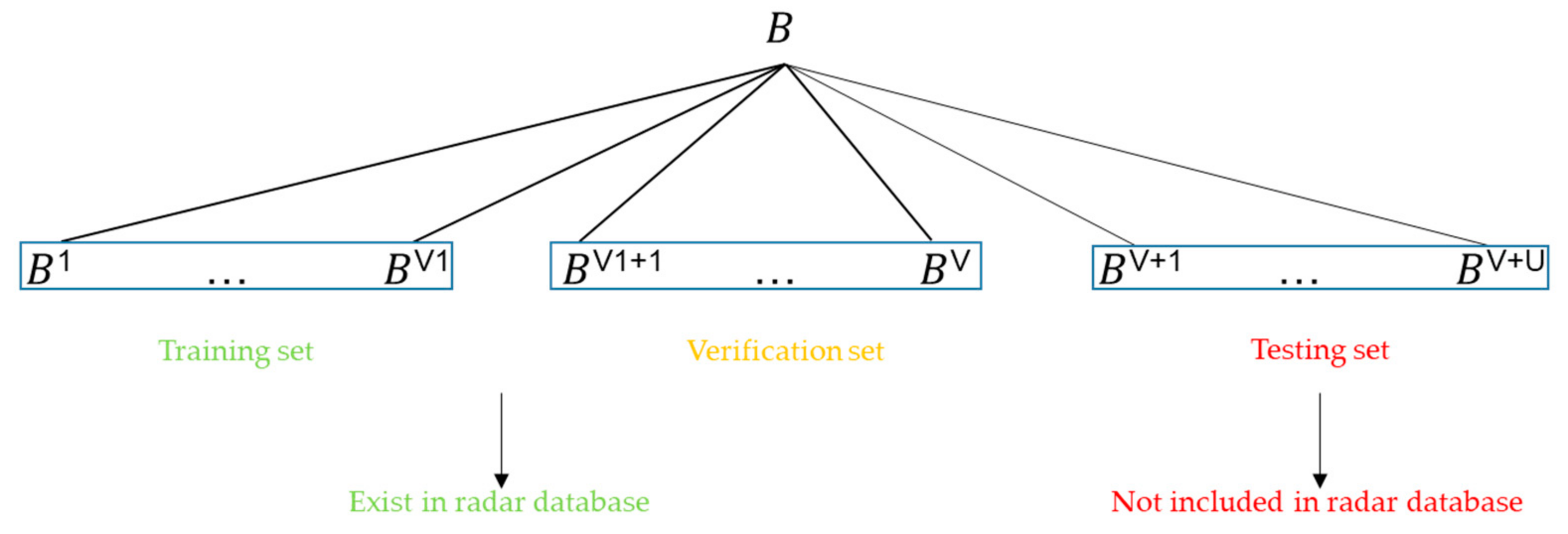
3.1. Dataset
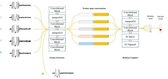
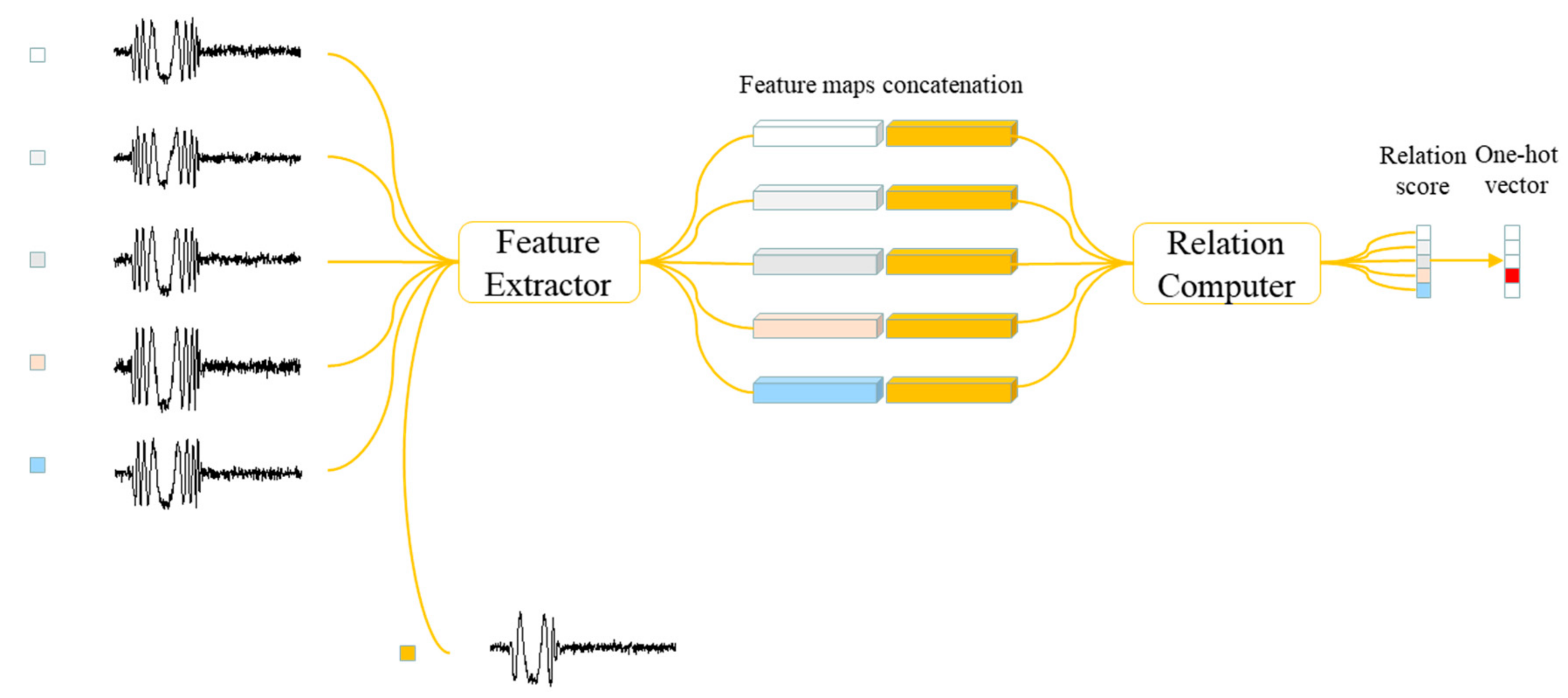
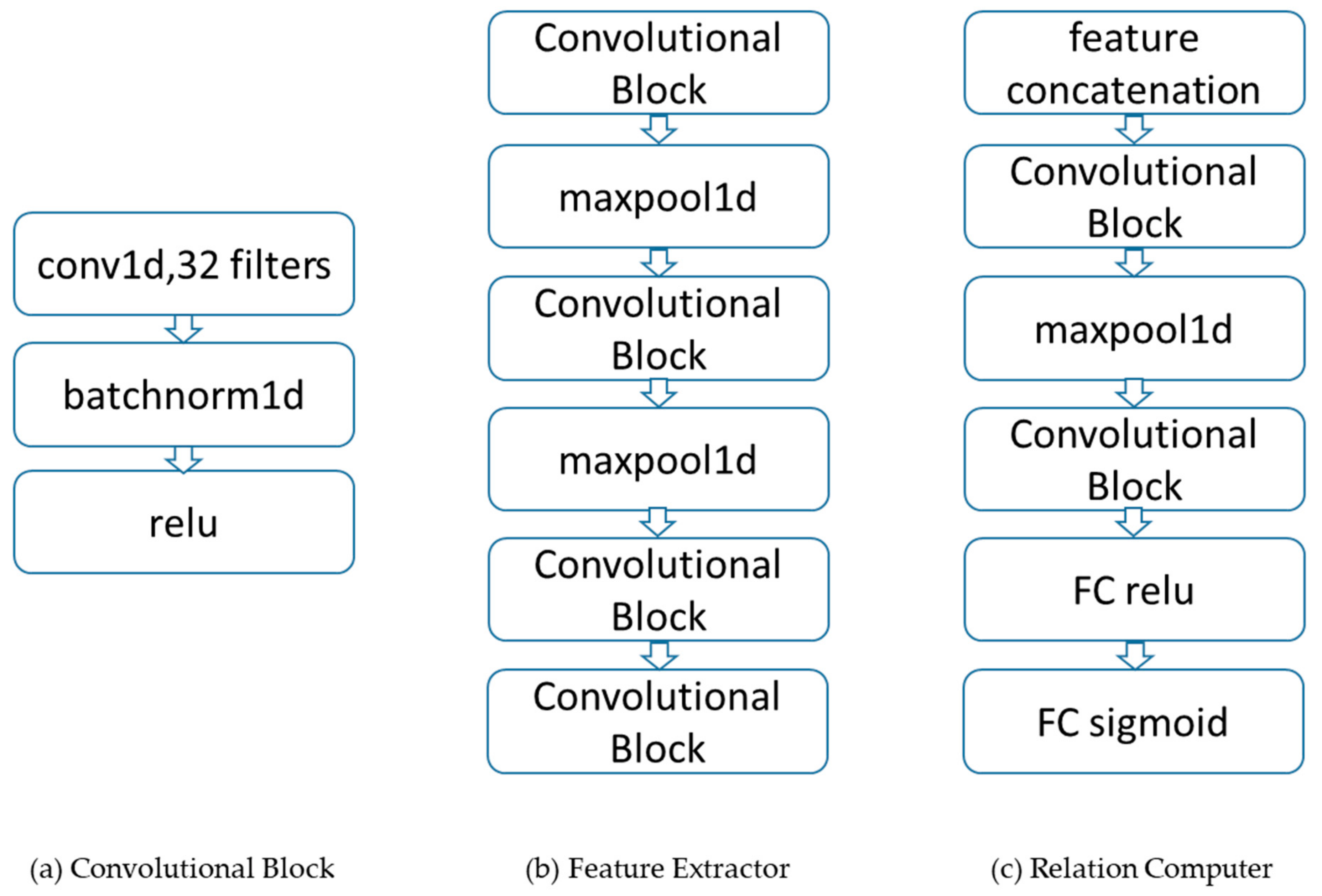
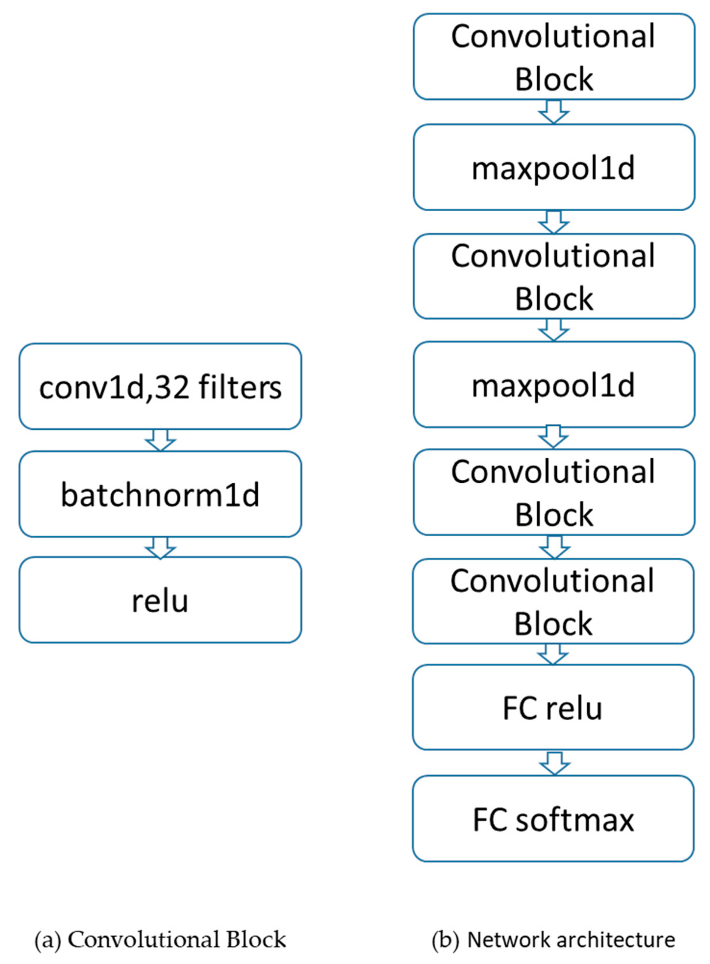
3.2. Network Architecture
3.3. Experiments
- (a)
- Extracting pulse envelope by Hilbert transform;
- (b)
- Moving average filtering for aliasing noise;
- (c)
- Normalization of pulse envelope;
- (d)
- Extracting “standard” envelope waveform by means of averaging;
- (e)
- Identification by the nearest neighbor classification method.
- (a)
- Segment and de-average the received signal;
- (b)
- Solve the third-order cumulative function of each signal;
- (c)
- Calculate the mean of the third-order cumulants of all signals;
- (d)
- Fourier transform the results of the previous step to obtain the bispectral diagonal slice;
- (e)
- Identification by the nearest neighbor classification method.
- (a)
- Segment and de-average the received signal;
- (b)
- Calculate the autocorrelation function of each signal;
- (c)
- Fourier transform the results of the previous step to obtain the ambiguity function;
- (d)
- Let the frequency offset be 0 to obtain the Zero-Slice feature of the ambiguity function;
- (e)
- Identification by the nearest neighbor classification method.
- (a)
- Rising time: the time of the pulse amplitude rising from 10% to 90%;
- (b)
- Falling time: the time of the pulse amplitude falling from 90% to 10%;
- (c)
- Pulse width: the time span between two nodes with a 50% pulse amplitude;
- (d)
- Rising angle: the angle between the time axis and the fitting line of the rising edge of the pulse;
- (e)
- Falling angle: the angle between the time axis and the fitting line of the falling edge of the pulse;
- (f)
- Frequency modulation angle: the angle between the regression line of the frequency waveform vector and the time axis.
4. Discussion
5. Conclusions
Author Contributions
Funding
Institutional Review Board Statement
Informed Consent Statement
Data Availability Statement
Acknowledgments
Conflicts of Interest
References
- Talbot, K.I.; Duley, P.R.; Hyatt, M.H. Specific Emitter Identification and Verification. Technol. Rev. J. Spring/Summer. 2003, pp. 113–133. Available online: http://jmfriedt.org/phase_digital/03SS_KTalbot.pdf (accessed on 12 June 2021).
- Xu, D. Research on Mechanism and Methodology of Specific Emitter Identification. Ph.D. Thesis, National University of Defense Technology, Changsha, China, 2008. [Google Scholar]
- He, M. Radar Countermeasure Information Processing, 1st ed.; Tsinghua University Press: Beijing, China, 2010. [Google Scholar]
- Langley, L.E. Specific emitter identification (SEI) and classical parameter fusion technology. In Proceedings of the WESCON’93, San Francisco, CA, USA, 28–30 September 1993; pp. 377–381. [Google Scholar]
- Wang, H.; Zhao, G.; Wang, Y. A specific emitter identification method based on front edge waveform of radar signal envelop. Aerosp. Electron. Warf. 2009, 25, 35–38. [Google Scholar]
- Liu, X.; Luo, P.; Li, G. Radar emitter individual identification based on fitting angle features and SVM. Comput. Eng. Appl. 2011, 47, 281–284. [Google Scholar]
- Xu, S.; Xu, L.; Xu, Z.; Huang, B. Individual radio transmitter identification based on spurious modulation characteristics of signal envelop. In Proceedings of the 2008 IEEE Military Communications Conference, San Diego, CA, USA, 16–19 November 2008; pp. 1–5. [Google Scholar]
- Zhang, G.; Huang, K.; Jiang, W.; Zhou, Y. Emitter feature extract method based on signal envelope. Syst. Eng. Electron. 2006, 28, 795–798. [Google Scholar]
- Rehman, S.U.; Sowerby, K.; Coghill, C. RF fingerprint extraction from the energy envelope of an instantaneous transient signal. In Proceedings of the 2012 Australian Communications Theory Workshop (AusCTW), Wellington, New Zealand, 30 January–2 February 2012; pp. 90–95. [Google Scholar]
- Wu, L.; Zhao, Y.; Feng, M.; Abdalla, F.Y.; Ullah, H. Specific emitter identification using IMF-DNA with a joint feature selection algorithm. Electronics 2019, 8, 934. [Google Scholar] [CrossRef] [Green Version]
- Feng, Z.; Zhang, D.; Zuo, M.J. Adaptive mode decomposition methods and their applications in signal analysis for machinery fault diagnosis: A review with examples. IEEE Access 2017, 5, 24301–24331. [Google Scholar] [CrossRef]
- Hall, J.; Barbeau, M.; Kranakis, E. Enhancing intrusion detection in wireless networks using radio frequency fingerprinting. In Proceedings of the IASTED International Conference on Communications, Internet, and Information Technology, St. Thomas, US Virgin Islands, USA, 22–24 November 2004; pp. 201–206. [Google Scholar]
- Hall, J.; Barbeau, M.; Kranakis, E. Detecting rogue devices in Bluetooth networks using radio frequency fingerprinting. In Proceedings of the 3rd IASTED International Conference on Communications and Computer Networks, Lima, Peru, 4–6 October 2006; pp. 108–113. [Google Scholar]
- Huang, Y.; Zheng, H. FSK radio fingerprints extraction based on distortions of instantaneous frequency. Telecommun. Eng. 2013, 53, 868–872. [Google Scholar]
- Padilla, P.; Padilla, J.L.; Valenzuela-Valdés, J.F. Radiofrequency identification of wireless devices based on RF fingerprinting. Electron. Lett. 2013, 49, 1409–1410. [Google Scholar] [CrossRef]
- Ye, W.; Yu, Z. Signal recognition method based on joint time-frequency radiant source. Electron. Inf. Warf. Technology 2018, 33, 16–19. [Google Scholar]
- Flamant, J.; Le Bihan, N.; Chainais, P. Time-frequency analysis of bivariate signals. Appl. Comput. Harmon. Anal. 2019, 46, 351–383. [Google Scholar] [CrossRef] [Green Version]
- Bertoncini, C.; Rudd, K.; Nousain, B.; Hinders, M. Wavelet fingerprinting of Radio-Frequency IDentification (RFID) tags. IEEE Trans. Ind. Electron. 2012, 59, 4843–4850. [Google Scholar] [CrossRef]
- Hippenstiel, R.D. Wavelet Based Approach to Transmitter Identification; NPS-EC-95-014; 1995. Available online: https://apps.dtic.mil/sti/citations/ADA304459 (accessed on 3 May 2021).
- Gao, J.; Kong, W.; Liu, J. Research on emitter modulation recognition of the adaptive PCA based on time-frequency analysis. Appl. Sci. Technol. 2018, 45, 33–37. [Google Scholar]
- Xie, Z.; Xu, L.; Ni, G.; Wang, Y. A new feature vector using selected line spectra for pulsar signal bispectrum characteristic analysis and recognition. Chin. J. Astron. Astrophys. 2007, 7, 565–571. [Google Scholar] [CrossRef]
- Cai, Z.; Li, J. Study of transmitter individual identification based on bispectra. J. Commun. 2007, 28, 75–79. [Google Scholar]
- Wang, H.; Zhang, T. Extraction algorithm of communication signal characteristics based on improved bispectra and time-domain Analysis. J. Signal Process. 2017, 33, 864–871. [Google Scholar]
- Yang, J.; Lu, X.; Zhou, Y. Transmitter individual identification based on polyspectra and support Vector Machine. Comput. Simul. 2010, 27, 349–353. [Google Scholar]
- Gong, Y.; Hu, G.; Pan, Z. Radio transmitter identification based on bispectra with tensor representation. In Proceedings of the 2010 2nd International Conference on Computer Engineering and Technology, Chengdu, China, 16–18 April 2010; Volume 3, pp. 294–298. [Google Scholar]
- Wang, H.; Zhang, T.; Meng, F. Specific emitter identification based on time-frequency domain characteristic. J. Inf. Eng. Univ. 2018, 19, 23–29. [Google Scholar]
- Wang, L. Analysis of subtle characteristics of low-frequency radiation. Master Thesis, Nanjing University of Aeronautics and Astronautics, Nanjing, China, 2014. [Google Scholar]
- Gui, Y.; Yang, J.; Lv, J. A fractal feature extraction algorithm based on empirical mode decomposition. J. Detect. Control. 2016, 38, 104–108. [Google Scholar]
- Zhang, J.; Wang, F.; Dobre, O.A.; Zhong, Z. Specific emitter identification via Hilbert-Huang transform in single-hop and relaying scenarios. IEEE Trans. Inf. Forensics Secur. 2016, 11, 1192–1205. [Google Scholar] [CrossRef]
- Huang, N.E.; Shen, Z.; Long, S.R.; Wu, M.C.; Shih, H.H.; Zheng, Q.; Yen, N.; Tung, C.C.; Liu, H.H. The empirical mode decomposition and the Hilbert spectrum for nonlinear and non-stationary time series analysis. Proc. R. Soc. A: Math. Phys. Eng. Sci. 1998, 454, 903–995. [Google Scholar] [CrossRef]
- Song, C.; Xu, J.; Zhan, Y. A method for specific emitter identification based on empirical mode decomposition. In Proceedings of the 2010 IEEE International Conference on Wireless Communications, Networking and Information Security, Beijing, China, 25–27 June 2010; pp. 54–57. [Google Scholar]
- Ha, Z.; Liu, X.; Cai, Q.; Wang, L. Study of specific emitter identification for ATC transponder. Electron. Inf. Warf. Technol. 2012, 27, 1–5. [Google Scholar]
- Liang, J.; Huang, Z.; Yuan, Y.; Huang, G.Q. A method based on empirical mode decomposition for identifying transmitter individuals. J. CAEIT 2013, 8, 393–397. [Google Scholar]
- Frei, M.G.; Osorio, I. Intrinsic time-scale decomposition: Time-frequency-energy analysis and real-time filtering of non-stationary signals. Proc. R. Soc. A: Math. Phys. Eng. Sci. 2007, 463, 321–342. [Google Scholar] [CrossRef]
- Li, X.; Duan, T.; Xu, W. ITD-based identification of signal fine features. J. Inf. Eng. Univ. 2014, 15, 570–575. [Google Scholar]
- Gui, Y.; Yang, J.; Lyu, J. Feature extraction algorithm based on intrinsic time-scale decomposition model for communication transmitter. Appl. Res. Comput. 2017, 34, 1172–1175. [Google Scholar]
- Ren, D.; Zhang, T.; Han, J. Approach of specific communication emitter identification combining ITD and nonlinear analysis. J. Signal Process. 2018, 34, 331–339. [Google Scholar]
- Ren, D.; Zhang, T.; Han, J.; Wang, H.H. Specific emitter identification based on ITD and texture analysis. J. Commun. 2017, 38, 160–168. [Google Scholar]
- Martis, R.J.; Acharya, U.R.; Tan, J.H.; Petznick, A.; Tong, L.; Chua, C.K.; Ng, E.Y.K. Application of Intrinsic Time-scale Decomposition (ITD) to EEG signals for automated seizure prediction. Int. J. Neural Syst. 2013, 23, 1350023. [Google Scholar] [CrossRef]
- An, X.; Jiang, D.; Chen, J.; Liu, C. Application of the intrinsic time-scale decomposition method to fault diagnosis of wind turbine bearing. J. Vib. Control. 2012, 18, 240–245. [Google Scholar] [CrossRef]
- Xu, Y.; Xie, Z.; Cui, L.; Wang, J. The feature extraction method of gear magnetic memory signal. Adv. Mater. Res. 2013, 819, 206–211. [Google Scholar] [CrossRef]
- Dragomiretskiy, K.; Zosso, D. Variational mode decomposition. IEEE Trans. Signal Process. 2014, 62, 531–544. [Google Scholar] [CrossRef]
- Chen, S.; Zheng, X. Research on mechanical fault diagnosis method of circuit breaker based on VMD energy entropy and support vector machine. Heilongjiang Electr. Power 2019, 41, 60–63. [Google Scholar]
- Meng, Q. Nonlinear Dynamical Time Series Analysis Methods and Its Application. Ph.D. Thesis, Shandong University, Shandong, China, 2008. [Google Scholar]
- Carroll, T.L. A nonlinear dynamics method for signal identification. Chaos: Interdiscip. J. Nonlinear Sci. 2007, 17, 023109. [Google Scholar] [CrossRef]
- Yuan, Y. Research on Key Technology of Communication Specific Emitter Identification. Ph.D. Thesis, National University of Defense Technology, Changsha, China, 2014. [Google Scholar]
- Zhu, S. Research on Applications of Chaotic Signal Processing in Specific Emitter Identification. Ph.D. Thesis, School of Information and Communication, Chengdu, China, 2018. [Google Scholar]
- Bihl, T.J.; Bauer, K.W.; Temple, M.A. Feature selection for RF fingerprinting with multiple discriminant analysis and using ZigBee device emissions. IEEE Trans. Inf. Forensics Secur. 2016, 11, 1862–1874. [Google Scholar] [CrossRef]
- Zhu, S.; Gan, L. Specific emitter identification based on visibility graph entropy. Chin. Phys. Lett. 2018, 35, 030501. [Google Scholar] [CrossRef]
- Xu, D.; Xu, H.; Lu, Q. A specific emitter identification method based on self-excitation oscillator model. Signal Process. 2008, 24, 122–126. [Google Scholar]
- Xu, Z.; Chen, Z.; Wang, J.; Xu, Y.L.; Kong, L. An improved method for emitter identification based on character of power amplifier. J. Nanjing Univ. Posts Telecommun. Nat. Sci. 2013, 33, 54–58. [Google Scholar]
- Huang, Y.; Zheng, H. Emitter fingerprint feature extraction method based on characteristics of phase noise. Comput. Simul. 2013, 30, 182–185. [Google Scholar]
- Man, P.; Ding, C.; Ren, W.; Xu, G. A Nonlinear Fingerprint-Level Radar Simulation Modeling Method for Specific Emitter Identification. Electronics 2021, 10, 1030. [Google Scholar] [CrossRef]
- Kingma, D.; Ba, J. Adam: A Method for Stochastic Optimization. Computer Science. 2014. Available online: https://arxiv.org/abs/1412.6980 (accessed on 12 January 2021).
- Fan, Y. The Feature Extraction of Radar Source and Radar Individual Identification. Master Thesis, Xidian University, Xi’an, China, 2017. [Google Scholar]
- Ren, L. Research on Emitter Fingerprint Identification and Fine Feature Extraction. Master Thesis, Harbin Engineering University, Harbin, China, 2012. [Google Scholar]
- Wang, L. On Methods for Specific Radar Emitter Identification. Ph.D. Thesis, Xidian University, Xi’an, China, 2011. [Google Scholar]
- Chen, J. Features Selection and Specific Emitter Identification of Radar. Master Thesis, Xidian University, Xi’an, China, 2013. [Google Scholar]

| Components | Main Design Parameters | Typical Values |
|---|---|---|
| Signal Source | Phase truncation bits | 12 |
| Amplitude quantization bits | 10 | |
| Integral nonlinearity | 3 LSB | |
| Differential nonlinearity | 0.5 LSB | |
| Mixer | Suppression of the alternate output sideband | −200 dB |
| RF to output rejection | −200 dB | |
| LO to output rejection | −200 dB | |
| LO to RF isolation | −200 dB | |
| RF to LO isolation | −200 dB | |
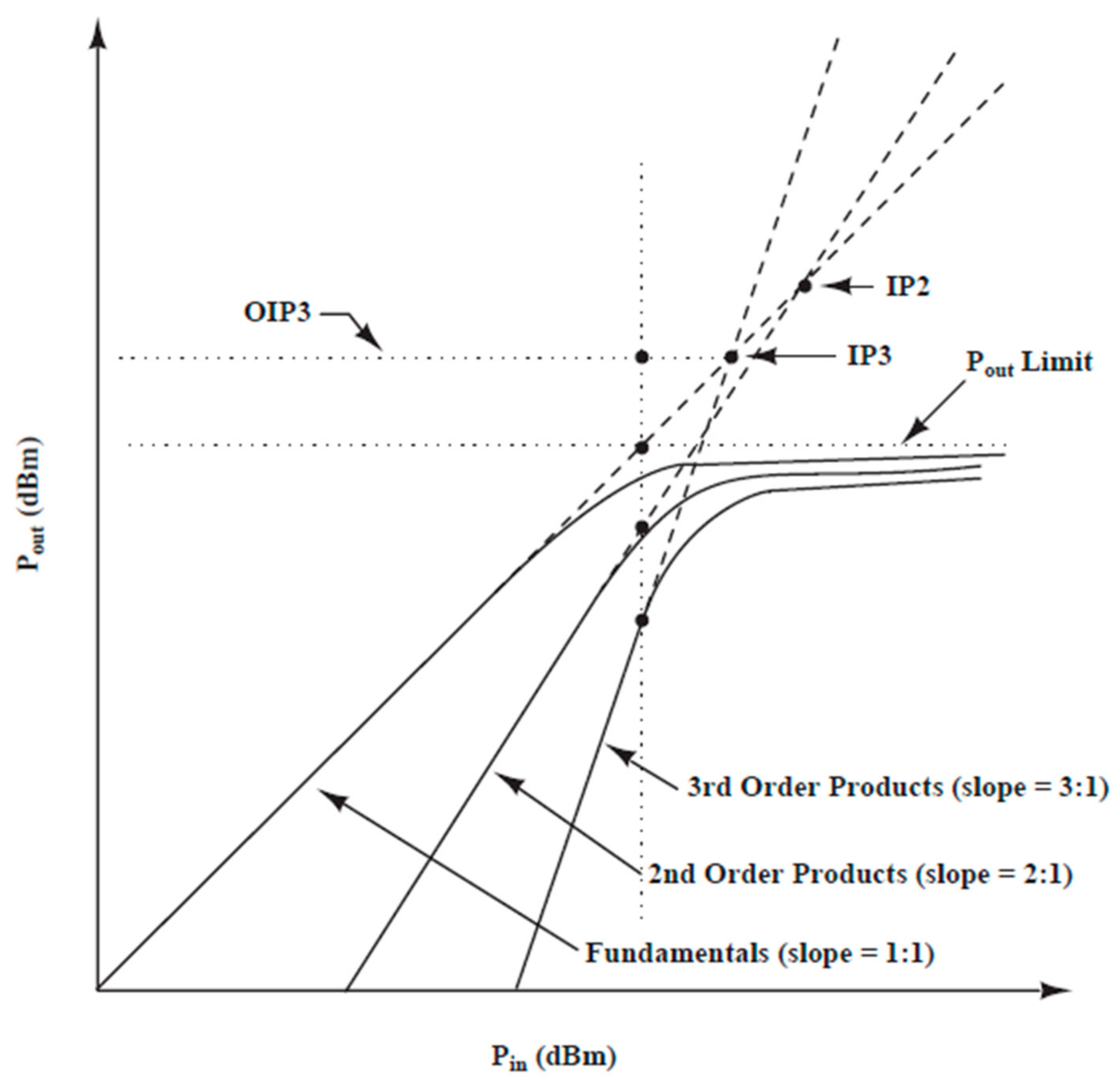
| Second-order truncation points | 40 dBm | |
| Third-order truncation points | 25 dBm | |
| Amplifier | 1 dB compression points | 17 dBm |
| Second-order truncation points | 20 dBm | |
| Third-order truncation points | 35 dBm | |
| Local Oscillator | Phase noise | [−85, −105, −110, −115, −135] |
| Changes in Working Parameters | Signal-to-Noise Ratio | Algorithm [55] | Algorithm [56] | Algorithm [57] | Algorithm [58] |
|---|---|---|---|---|---|
| constant | 30 dB | 92.2% | 89.9% | 99.8% | 100.0% |
| 20 dB | 67.8% | 67.4% | 87.8% | 90.1% | |
| 10 dB | 37.2% | 37.0% | 56.0% | 35.0% |
| Changes in Working Parameters | Signal-to-Noise Ratio | Algorithm [55] | Algorithm [56] | Algorithm [57] | Algorithm [58] |
|---|---|---|---|---|---|
| 30 dB | 88.2% | 88.4% | 100% | 99.8% | |
| 20 dB | 61.0% | 57.8% | 91.2% | 87.54% | |
| 10 dB | 37.8% | 30.4% | 57.6% | 36.6% | |
| 30 dB | 46.2% | Unrecognized | Unrecognized | Unrecognized | |
| 20 dB | 32.2% | ||||
| 10 dB | 23.8% | ||||
| 30 dB | Unrecognized | Unrecognized | Unrecognized | 28.1% | |
| 20 dB | 26.0% | ||||
| 10 dB | 24.5% | ||||
| 30 dB | Unrecognized | 21.2% | Unrecognized | Unrecognized | |
| 20 dB | 27.6% | ||||
| 10 dB | 31.2% | ||||
| 30 dB | Unrecognized | Unrecognized | Unrecognized | 20.1% | |
| 20 dB | 23.2% | ||||
| 10 dB | 24.6% | ||||
| 30 dB | 22.3% | Unrecognized | Unrecognized | 20.4% | |
| 20 dB | 25.5% | 23.2% | |||
| 10 dB | 30.0% | 26.9% | |||
| 30 dB | 21.2% | Unrecognized | Unrecognized | Unrecognized | |
| 20 dB | 25.4% | ||||
| 10 dB | 29.8% |
| Signal-to-Noise Ratio | |||||||
|---|---|---|---|---|---|---|---|
| 10 dB | 39.2% | 33.5% | 26.8% | 36.2% | 35.1% | 31.3% | 29.1% |
| 20 dB | 49.6% | 41.2% | 30.0% | 45.1% | 45.9% | 40.0% | 28.4% |
| 30 dB | 51.2% | 43.3% | 40.9% | 48.4% | 48.6% | 43.5% | 30.3% |
| Signal-to-Noise Ratio | |||||||
|---|---|---|---|---|---|---|---|
| 10 dB | 100.0% | 77.6% | 78.4% | 72.8% | 71.4% | 92.2% | 70.2% |
| 20 dB | 100.0% | 82.4% | 92.4% | 78.0% | 80.5% | 96.6% | 73.6% |
| 30 dB | 100.0% | 96.2% | 99.2% | 83.4% | 84.5% | 99.8% | 81.3% |
Publisher’s Note: MDPI stays neutral with regard to jurisdictional claims in published maps and institutional affiliations. |
© 2021 by the authors. Licensee MDPI, Basel, Switzerland. This article is an open access article distributed under the terms and conditions of the Creative Commons Attribution (CC BY) license (https://creativecommons.org/licenses/by/4.0/).
Share and Cite
Man, P.; Ding, C.; Ren, W.; Xu, G. A Specific Emitter Identification Algorithm under Zero Sample Condition Based on Metric Learning. Remote Sens. 2021, 13, 4919. https://doi.org/10.3390/rs13234919
Man P, Ding C, Ren W, Xu G. A Specific Emitter Identification Algorithm under Zero Sample Condition Based on Metric Learning. Remote Sensing. 2021; 13(23):4919. https://doi.org/10.3390/rs13234919
Chicago/Turabian StyleMan, Peng, Chibiao Ding, Wenjuan Ren, and Guangluan Xu. 2021. "A Specific Emitter Identification Algorithm under Zero Sample Condition Based on Metric Learning" Remote Sensing 13, no. 23: 4919. https://doi.org/10.3390/rs13234919
APA StyleMan, P., Ding, C., Ren, W., & Xu, G. (2021). A Specific Emitter Identification Algorithm under Zero Sample Condition Based on Metric Learning. Remote Sensing, 13(23), 4919. https://doi.org/10.3390/rs13234919